Título artículo / Títol article:
Improving Hyperspectral Pixel
Classification With Unsupervised Training
Data Selection
Autores / Autors
O. Rajadell, P. García-Sevilla, Viet Cuong
Dinh, R.P.W. Duin
Revista:
Geoscience and Remote Sensing Letters,
IEEE
Versión / Versió:
Versió post-print
Cita bibliográfica / Cita
bibliogràfica (ISO 690):
RAJADELL, Olga, et al. Improving
Hyperspectral Pixel Classification With
Unsupervised Training Data Selection.
Geoscience and Remote Sensing Letters,
IEEE
, 2014, vol. 11, no 3, p. 656-660.
url Repositori UJI:
Improving hyperspectral pixel classification with
unsupervised training data selection
Olga Rajadell, Pedro Garc´ıa-Sevilla, Viet Cuong Dinh and Robert P.W. Duin
Abstract—An unsupervised method for selecting training data is suggested here. The method is tested by applying it to hyperspectral land-use classification. The data set is reduced using an unsupervised band selection method and then clustered with a non parametric cluster technique. The cluster technique provides centers of the clusters and those are the samples selected to compose the training set. Both the band selection and the clustering are unsupervised techniques. Afterwards an expert labels those samples and the rest of unlabeled data can be classified. The inclusion of the selection step, although unsupervised, allows to select automatically the most suitable pixels to build the classifier. This reduces the expert effort because less pixels need to be labeled. However, the classification results are significantly improved in comparison with results obtained by a random selection of training samples, in particular for very small training sets.
I. INTRODUCTION
Segmentation and classification are well known issues in image processing that are lately faced as a single problem by using pixel classification. For classification, expert labeling is needed to train the system to later classify unlabeled samples. Some authors work in a supervised scenario where prior knowledge is available and training data is selected within each class [1] [2]. Active learning techniques have also been ap-plied. In these, the expert collaboration improves progressively the training data [3] [4]. In both cases, the way the training data is first selected is a concern generally solved by randomly picking among the unlabeled data. This is unsupervised but not very efficient. Randomly distributed samples can lie in non interesting areas and reducing the size of the training set may make the training data non representative. On top of that, expert collaboration is expensive. To face both problems we suggest to provide the system with the most interesting samples from the beginning. The traditional randomly selected training set is thereby replaced by a selective choice.
In unsupervised scenarios, data analysis techniques are widely used for finding relevant data when no prior knowledge is available. Among them, clustering techniques allow to divide data into groups of similar samples. A very large number of clustering techniques is available but some of them rely upon a prior knowledge, such as the number of clusters and the shape of clusters in the feature space (often elliptical). When dealing with an arbitrarily structured feature space, only nonparametric methods are applicable since no model Olga Rajadell and Pedro Garc´ıa-Sevilla are with the University Jaume I, Spain, within the Institute of New Imaging Technologies (http://www.init.uji.es). Viet Cuong Dinh and Robert P.W. Duin are with Delft University of Technology, PRLab, The Netherlands. Viet Cuong Dinh is also with of CTR, Villach, Austria.
assumption have to be made [5]. Clustering algorithms have successfully been applied to image segmentation in various fields and applications [6]. Fully unsupervised procedures often have insufficiently accurate segmentation results. For such a reason, a hybrid scenario between supervised and unsupervised techniques is of high interest. In this case, the methods applied use a small set of labels to train a classifier. Because labeling is neither fast nor cheap, the fewer labeled data the system needs the better [7].
The contribution of this paper is the introduction of a method to select the training data. The suggested method is tested for hyperspectral landscape image classification and compared with a random selection of the training set. Results based on a selective choice of the training set outperform those achieved with randomly picked training data, mainly when a very small number of labeled samples is used. The scheme is presented in Section II with a focus on the selection method. Results will be shown over the dataset presented in Section III and analyzed in Section IV. Section V are conclusions.
II. CLASSIFICATION SCHEME
Comaniciu et al. states in [8] that vision tasks can be improved if they are supported by more reliable data. Nowa-days databases used for segmentation and classification of hyperspectral satellite images are fairly reliable in terms of spectral and spatial resolution. Therefore, we can consider that our feature space representation of the data is reliable. However, training sets are often built by randomly picking a percentage of samples. We suggest to make an unsupervised selection of the training samples based on the analysis of the feature space. This aims at providing an improved training set. The whole classification scheme proceeds as follows:
1) A band selection method is used. With it the data set is reduced to a smaller set of bands. This set is less correlated than the original while it keeps as much information as possible. We used the WALUMI band se-lection method [9], but any other band sese-lection method that fulfils that requirement could be used instead. 2) A clustering procedure is applied over the reduced
dataset. The centers of the clusters found form the selected training set. A non-parametric clustering tech-nique is used and prior knowledge is not needed. 3) The expert is involved once, after the selection, to
provide the corresponding labels of the selected samples. In this paper the expert will be simulated by checking the corresponding labels on the groundtruth.
4) A classifier is built using the training set defined before. Although the clustering is performed using spectral
used independently to the type of features used for classifying.
A. Mode seeking clustering
Mode seeking clustering is a well known clustering princi-ple for image segmentation. Based on a given set of objects, in case of images these are the pixels, a non-parametric estimate of the probability density function (pdf) is made. The modes of this pdf correspond to the clusters. In a gradient search all objects are used as a starting point and objects ending up in the same mode belong to the same cluster. Neither the number of clusters nor their shape has to be predefined.
The most popular mode seeking procedure is the mean shift algorithm [10] [11]. It is based on a Parzen kernel density estimate of the pdf. In contrast to the classic K-means clustering [12], or the more advanced Mixture-Of-Gaussian density estimates there are no embedded assumptions on an underlying Gaussian distribution of the data [10] [8]. In the mean shift algorithm the direction of the local gradient is found by a shift of the mean of the local mean when the distances to the objects in a local neighborhood are weighted by the chosen kernel. This procedure works well for the segmentation of color images, especially when some spatial information is included in features representing the pixels [8]. Problems with mean shift are that the modes as well as the convergence are not sharply defined. Thereby, separate nearby modes may be found that are erroneously not merged. Moreover, formally all pixels have to be used as a starting point, which is very time consuming.
Another algorithm based on mode seeking is kNN mode seeking. Instead of the Parzen kernel density estimate it is entirely based on the distances to thek-th neighbor. It can be traced back to a proposal by Koontz et al. in 1977 [13]. It has been around in the Matlab toolbox PRTools [14] for 20 years. Recently it has been redefined [15] and compared with mean shift. The procedure can be summarized as:
Do for all objects:
1) Find its knearest neighbors.
2) Use the distance to the k-th neighbor as a measure for the density (in fact one over the distance).
3) Define a pointer to the object with the highest density in thek-neighborhood.
4) Follow from all objects the pointers until objects are reached that point to themselves: the modes.
Various implementations are studied. We used one that is based on an approximate nearest neighbor search [16]. It performs the above algorithm for clustering 10366 objects in 5 dimensions with k=100 in 1.4 seconds and with k=10 in less than a second (0.7) on a standard PC (Intel Core Duo 2GHz, with 4GB of RAM). Its computational complexity is about O(kn2) for data sets with n objects. The dependency on the dimensionality is heavily problem dependent due to the approximate nearest neighbor. Advantages of this algorithm over mean shift are that it is much faster and converges exactly to modes that correspond with objects (pixels). Moreover it can handle high dimensional spaces and finds solutions for sets of
k-value in the set.
B. The role of spatial coordinates
The specific task targeted here is the classification of land cover images. In this type of images, the samples are pixels and the classes the different areas in the image. Thus, samples within the same class are spatially connected (class connection principle or smoothness). This is an advantage because it adds extra information to the spectral information provided by sensors. However, it can happen that a class is located in more than one spatial location. In such a case, even being the same class, the characteristics of their samples can differ due to different lighting or soil conditions in the different locations. The clustering algorithm chosen searches for local density maxima where the density function has been calculated using the distances for each sample in its k neighbourhood. A smaller k results in a higher number of clusters, that is helpful if we aim to select more samples from different areas. However, unique large areas would also have many samples selected within the same region that are unnecessary (redundant training data). On the contrary, bigger k would provide fewer selected samples for big areas but smaller areas or different locations of the same class would be missed instead.
We suggest to incorporate spatial information to the selec-tion algorithm. Like this the clustering will also take into ac-count their spatial connectivity. This has already been done in literature [17] by simply adding the spatial coordinates to the feature vector of each pixel. By adding the coordinates within the distance computation, samples nearby will have a higher probability of being clustered together and the opposite for spatially remote samples even if they belong to the same class. Note that coordinates are only used for this clustering step and only the spectral information (without the coordinates) or features derived from the spectral information are used in the classification step. This allows a fair comparison with several methods proposed by other authors and the random selection method included in the paper. That is, the features used in the classification step for the mode selection method and for the random selection method are exactly the same. The only difference lies in how the training set is built.
C. Spectral-spatial features
The contribution of this paper is a training selection method. Such a method should point out which samples are significant for training independently of the features used for classi-fication afterwards. To that end, we suggest to switch the features for classification, using the same selected samples for training in order to show that this selection still outperforms a random pick selection. We choose a different type of features, spatial features extracted by filtering suggested in [18]. These are obtained by filtering the input image with a set of two-dimensional Gabor filters. The outputs of each pixel in the im-age forms its feature vector. Each Gabor filter is characterized by a preferred orientation and a preferred spatial frequency (scale) so this features characterized the texture contained in the image.
III. DATASET
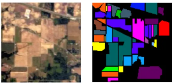
The dataset used in the experiments is widely known in the field. Hyper-spectral image 92AV3C (Fig. 1) was provided by the Airborne Visible Infrared Imaging Spectrometer (AVIRIS) and acquired over the Indian Pine Test Site in Northwestern Indiana in 1992. From the 220 bands that composed the image, 20 are usually ignored because of the noise (the ones that cover the region of water absorption or with low SNR) [19]. The image has a spatial dimension of 145×145 pixels. Spatial resolution is 20m per pixel. Classes range from 20 to 2468 pixels. In it, three different growing states of soya can be found, together with other three different growing states of corn. Woods, pasture and trees are the bigger classes in terms of number of samples (pixels). Smaller classes are steel towers, hay-windrowed, alfafa, drives, oats, grass and wheat. In total, the dataset has 16 labeled classes.
Fig. 1. AVIRIS database color composition and groundtruth.
IV. RESULTS
For all experiments, clustering is carried out using different values of the parameterkto get different sizes of training sets (selected samples). Notice that this is not an iterative process. The clustering is performed once and, as a consequence of the value of the parameterk, a number of samples is selected. The expert labels these samples and the classification is performed using only that labeled data as training and the rest as test. Plots in Fig. 2, 3, and 4 are represented in terms of error rate versus number of labeled samples provided for training. They represent the improvement of the classification when increasing the amount of labeled data.
A K-NN with K = 1 classifier has been used (not to be confused with the k-NN mode seeking procedure used for clustering). This is not an arbitrary choice. Because the clustering procedure used is based on densities determined by distances, the local maxima (the pixels used for training) correspond to samples which have many objects in their direct neighborhood. Small classes, or uni-modal classes may be represented by a single training point, so larger values of K
are not possible.
The dataset was reduced to different number of selected bands using WaLuMi band selection method. The bands selected used for the experiments carried out are presented in Table I.
A. Classification results
In Fig. 2 the learning curves for a different number of spectral bands are presented in both cases, selecting samples
no. of bands selected bands 3 4, 67, 87
10 4, 24, 51, 67, 78, 87, 99, 118, 129, 182 20 4, 15, 24, 33, 35, 36, 41, 51, 67, 77
79, 87, 95, 99, 111, 118, 129, 172, 182, 204
TABLE I
SELECTED BANDS USINGWALUMI FORAVIRISDATASET.
with the method and picking the same amount of samples at random. It is noticeable that in all cases, when selecting the training set, the classification rate outperforms the result obtain when the same amount is picked at random. When a small training set is used the difference between the the error rate selecting and not selecting is 0.3, whereas it decreases to 0.15 when the training set grows. This happens because the higher the number of samples is picked, the chances of randomly select samples from all classes are bigger. Also when the number of samples to select is very small random is very unstable. Note that no advantage is obtained in involving a higher number of spectral bands in the process. However, the difference between using10 and20 bands is an increase of 10 features in the feature vector. The main reason for selecting information is that, once known which are the most informative bands for a given sensor, further repetitions of the same task can be performed dismissing information that was proved to be redundant for that task using that sensor.
Fig. 2. Learning curves for different number of spectral features comparing the result selecting the training set with the corresponding number of training samples picked at random.
For the next experiment, the spatial-textural type of features is also used for classification. Note that the selection is the same and the target is to validate that the same training selection result improves the random selection being indepen-dently of the features used. These other features are computed from each band independently and8features are obtained per band. In Fig. 3 we show the learning curves obtained for the experiments that use 3 and 10 bands. Despite the difference between the size of the feature vector (24for 3 bands and 80
for10), no performance increase is noticed. As a summary also the difference in the error rate caused by changing the features for classifying (10 spectral and 24 spectral/spatial features) can be observed in Figure 4. Note how in both cases the error rate obtained using the random selection stays above the
classifica-that both sets of features start around the same error rate but the difference is quickly introduced when more samples are included. When using spectral/spatial features the error rate decreases considerably. The characterization improvement that these features introduce, together with providing representative labeled data, obtains a fairly good well classified area with a relatively small amount of labeled data.
Fig. 3. Learning curves for different number of spectral bands using spectral/spatial features. Results selecting the training set are compared with the same amount of samples picked at random.
Fig. 4. Comparison between two types of features. Learning curves for the classification results using selection of the training and random pick.
B. Analysis per class
Note that because classes are highly unbalanced, an in-crease in the performance is wanted when it represents an improvement for all classes and, in this case, large classes have a higher impact on the overall accuracy. In Table II the error rate per class is shown. The results obtained with
3.5%of labeled samples are comparable, in terms of per class accuracy, with results obtained in other scenarios using 10%
of random labeled samples for training [1] or a fixed number of labeled samples per class (50 samples per class, 15 for small ones) [20]. This last approach favors small classes in comparison with the unsupervised selection method presented here. The number of samples per class used in the training set is here unsupervised and no prior knowledge is used.
is better than experiments where the training selection is not used. Stone-steel towers, alfalfa, grass/pasture-mowed have error rates around 0.10 with only one or two samples for training. Other classes usually dismissed in the classification experiments because of their size [2] [21] like wheat, corn and Bldg-Grass-Tree-Drives have error rates of0.07,0.14and
0.01using only six, nine and ten labeled samples.
0.6%of training data 3.5%of training data classes training/total error training/total error Stone-steel towers 1/95 0.04 2/95 0.05 Hay-windrowed 4/489 0.03 19/489 0.03 Corn-min till 6/834 0.33 27/834 0.17 Soybeans-no till 7/968 0.10 29/968 0.11 Alfalfa 1/54 0.07 2/54 0.11 Soybeans-clean till 4/614 0.40 21/614 0.12 Grass/pasture 4/497 0.14 14/497 0.21 Woods 9/1294 0.08 47/1294 0.04 Bldg-Grass-Tree-Drives 4/380 0.002 10/380 0.01 Grass/pasture-mowed 0/26 1 1/26 0.04 Corn 1/234 0.38 9/234 0.14 Oats 0/20 1 0/20 1 Corn-no till 8/1434 0.25 44/1434 0.13 Soybeans-min till 11/2468 0.21 90/2468 0.04 Grass/trees 5/747 0.11 28/747 0.06 Wheat 2/212 0.15 6/212 0.07 Overall error 0.26 0.12 TABLE II
ACCURACY PER CLASS FOR THE16CLASSES CLASSIFICATION OF THE AVIRISDATASET SELECTING THE TRAINING SET OVER THE SPECTRAL
FEATURES CONCATENATED WITH THE SPATIAL COORDINATES AND CLASSIFYING USING SPATIAL-SPECTRAL FEATURES.
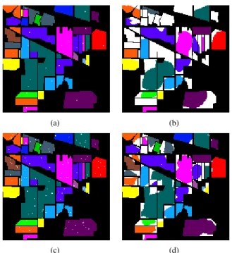
For an overview of the per class result, observe in Fig. 5.(a)(c) the selected training set (white points represented on the groundtruth) and the corresponding per class results Fig. 5.(b)(d)(where the color areas are well-classified pixels and the white ones miss-classified pixels). Both cases result from selecting training data by clustering over 10 spectral features plus two spatial coordinates, label the samples se-lected and use them as training set for a KNN classifier, replacing the spectral features by 24 spatial-spectral features for classification.
The case of a reduced number of training samples, Fig. 5(first row), demonstrates that one sample is needed to recognize a class (those areas where a mode is not found are dismissed in the classification). Leaving aside the misclassified areas, observe that those where a sample is labeled provide a well-classified region around them with 23 samples of training (only a0.22%of the dataset). In a scenario with a very reduced amount of labeled data, it should be considered the possibility that the expert corrects the loss by adding training samples of a region that has not been detected. For the bigger training set size, Fig. 5(second row) with only 104 samples, fulfils that classes distributed in different regions have samples for each of those regions and big regions have several labeled samples distributed along the fields, maximizing the classified area.
V. CONCLUSIONS
A method for selecting the training set has been suggested to replace the common random pick selection. This is useful when no prior knowledge is available and expert collaboration
(a) (b)
(c) (d)
Fig. 5. Classification results using 24 spectral/spatial features derived from 3 bands. (a) 23 selected training samples shown in white. (b) representation of misclassified pixels in white, error rate was 0.41. (c) 104 selected training samples shown in white. (d) representation of misclassified pixels in white, error rate of 0.147.
is limited. Thanks to the selection of the training set, only relevant samples can be shown to the expert to be labeled. In this sense, expert collaboration is reduced while performance has shown to be raised in comparison with random selection. The method is based on an unsupervised study of the data by a clustering technique. Besides, a spatial improvement was suggested to avoid redundant training data by including spatial coordinates in the clustering process. This forced clusters to merge or split according to the class connection principle. Thus, the training set is representative and free of redundancies. The selection has shown to be valid for building a classifier even if the features are changed. It was shown that textural-spatial features can also benefit from this selection scheme and achieve same results with less training data. Indeed, results shown outperform results of classification methods in literature that use a random selection of their training set. On the top of that, the process does not need large amounts of data since it has been shown that not all spectral bands and not a high number of features were needed in our experiments.
ACKNOWLEDGMENT
Thanks to Fundaci´o Caixa Castell´o-Bancaixa for funding by grant FPI PREDOC/2007/20. Also to the Spanish Ministry of Science and Innovation for supporting in projects CSD2007-00018 (Consolider Ingenio 2010), AYA2008-05965-C04-04 and MTM2009-14500-C02-02.
REFERENCES
[1] Y.Tarabalka, J.Chanussot, and J.A.Benediktsson, “Segmentation and classification of hyperspectral images using watershed transformation,” Patt.Recogn., vol. 43, no. 7, pp. 2367–2379, 2010.
[2] A. Plaza et al., “Recent advances in techniques for hyperspectral image processing,” Remote sensing of environment, vol. 113, pp. 110–122, 2009.
[3] D. Tuia, F. Ratle, F. Pacifici, M. Kanevski, and W. Emery, “Active learn-ing methods for remote senslearn-ing image classification,”IEEE Transactions on Geoscience and Remote Sensing, vol. 47, no. 7, pp. 2218 –2232, july 2009.
[4] J. Li, J. Bioucas-Dias, and A. Plaza, “Semisupervised hyperspectral image segmentation using multinomial logistic regression with active learning,” IEEE Transactions on Geoscience and Remote Sensing, vol. 48, no. 11, pp. 4085 –4098, nov. 2010.
[5] A. Jain, R. Duin, and J. Mao, “Statistical pattern recognition: a review,” IEEE Trans. on Pattern Analysis and Machine Intelligence, vol. 22, no. 1, pp. 4 –37, jan 2000.
[6] M. Filippone, F. Camastra, F. Masulli, and S. Rovetta, “A survey of kernel and spectral methods for clustering,”Pattern Recognition, vol. 41, no. 1, pp. 176 – 190, 2008.
[7] A. Ng, M. Jordan, and Y. Weiss, “On spectral clustering: Analysis and an algorithm,”Advances in Neural Information Processing Systems, vol. 14, no. 5, pp. 849 –856, 2002.
[8] D. Comaniciu and P. Meer, “Mean shift: a robust approach toward feature space analysis,”IEEE Trans. on Pattern Analysis and Machine Intelligence, vol. 24, no. 5, pp. 603 –619, may 2002.
[9] A. Mart´ınez-Us´o, F. Pla, and P. Garc´ıa-Sevilla, “Clustering-based hy-perspectral band selection using information measures,”IEEE Trans. on Geoscience & Remote Sensing, vol. 45, pp. 4158–4171, 2007. [10] Y. Cheng, “Mean shift, mode seek, and clustering,”IEEE Transaction
on Pattern Analysis and Machine, vol. 17, no. 8, pp. 790 –799, Aug. 1995.
[11] K. Fukunaga and L. Hostetler, “The estimation of the gradient of a density function, with applications in pattern recognition,” IEEE Transactions on Information Theory, vol. 21, no. 1, pp. 32–40, 1977. [12] R. Duda and P. Hart,Pattern classification. John-Wiley and Sons, 2001. [13] W. Koontz, P. Narendra, and K. Fukunaga, “A graph-theoretic approach to nonparametric cluster analysis,” IEEE Transactions on Computer, vol. 25, pp. 936–944, 1976.
[14] R. Duin, D. de Ridder, P. Juszczak, C. Lai, P. Paclik, E. Pekalska, and D. Tax, “Prtools4,” 2010. [Online]. Available: http://prtools.org [15] R. Duin, A. Fred, M. Loog, and E. Pekalska, “Mode seeking clustering
by knn and mean shift evaluated,” inSSPR SPR 2012 Lecture Notes in Computer Science, vol. 7626. Springer, 2012, pp. 51–59.
[16] S. Arya, D. M. Mount, N. S. Netanyahu, R. Silverman, and A. Y. Wu, “An optimal algorithm for approximate nearest neighbor searching in fixed dimensions,” Journal of the ACM, vol. 45, no. 6, pp. 891–923, 1998.
[17] N. Pal and S. Pal, “A review on image segmentation techniques,”Pattern Recognition, vol. 26, pp. 1277 – 1294, 1993.
[18] O. Rajadell, P. Garc´ıa-Sevilla, and F. Pla, “Spectral-spatial pixel char-acterization using gabor filters for hyperspectral image classification,” IEEE Geoscience & Remote Sensing Letters, vol. 10, no. 4, 2013. [19] D. A. Landgrebe, Signal Theory Methods in Multispectral Remote
Sensing, 1st ed. Hoboken, NJ: Wiley, 2003.
[20] Y.Tarabalka, J.Chanussot, and J.A.Benediktsson, “Segmentation and classification of hyperspectral images using minimum spanning forest grown from automatically selected markers,”IEEE Trans. Systems, Man, and Cybernetics, vol. 40, no. 5, pp. 1267 –1279, oct. 2010.
[21] G.Camps-Valls and L.Bruzzone, “Kernel-based methods for hyperspec-tral image classification,”IEEE Trans. on Geoscience & Remote Sensing, vol. 43, pp. 1351–1362, 2005.