Crowding-out Hypothesis in a Vector Error Correction
Framework: A Case Study of Pakistan
KALIM HYDER
I. INTRODUCTION
Under the umbrella of the IMF stabilisation programmes, Pakistan has pursued a policy of fiscal consolidation since 1988. A look at the budget deficit from 1988 onwards reveals that the policy has only been marginally successful. Even this fragile accomplishment of the Fund-based programme has been achieved at a much greater cost: the reduction in budget deficit has only been materialised because of the curtailment of development expenditure component of total fiscal outlays [Social Policy and Development Centre (2001)]. Economic theory suggests that development expenditure component of fiscal outlays, which also equals net investment by the public sector,1 has a significant relationship with both the rate of private investment and economic growth. If public investment increases, fewer funds will be available for private investment. Competition will thereby drive the interest rates up leading to lower level of private investment. Neo-classicals believe that this process will only result in a redistribution of gross national between the public and the private sector and the rate of economic growth will remain intact. On the other hand, Keynesians argue that the multiplier effect of higher public spending will be larger as compared to the induced negative effect of reduced private investment on the rate of economic activity and, therefore, gross national product will increase. The two views have traditionally been termed as the full crowding-out and the partial crowding-out hypotheses2 respectively [Abel and Bernanke (1992)].
Kalim Hyder is based at the Social Policy and Development Centre, Karachi.
1In Pakistan, Public investment is constructed primarily by economic activity as well as by capital
assets. It comprises expenditures incurred on the acquisition of fixed assets, replacement, additions and major improvements of fixed capital viz. land improvement, buildings, civil and engineering works, machinery, transport equipment and furniture and fixtures. While development expenditures refer to the expenditures incurred on the developmental activities.
2Theoretical models do not make the distinction between the consumption component of
government expenditure and the investment component. They simply refer to total government expenditure on goods and services. A difference, however, must be made because empirically, both these components have different types of effects on GNP and its growth.
Economic theory, therefore, suggests that pursuing the IMF based stabilisation programme is only defendable if the neo classical belief is correct. In this paper, we test whether this is true in the case of Pakistan or not. We seek to provide the evidence that is required by the economic managers to decide whether to increase public investment or target the budget deficit instead to boost the economy.
The crowding out hypothesis has so far been tested in Pakistan by analysing the impact of budget deficit on the interest rates [Ahmed (1994); Khan and Iqbal (1991); Burney and Yasmeen (1989); Haque and Montiel (1991, 1993)]. Some of these studies provide evidence of a negative relationship between budget deficit and interest rates implying that policy-makers should increase public spending [Ahmed (1994); Khan and Iqbal (1991)]. Others connote a support for the crowding out hypothesis based on positive association between interest rates and budget deficit [Haque and Montiel (1991, 1993)]. Although this testing mechanism provides a direct way for testing in favour of or against crowding out, it cannot simplistically be applied to Pakistan, as private investment in Pakistan is not significantly related to interest rates.3 A better way to test for crowding out would be to explore the dynamic interaction between public and private investment and economic growth [Barth and Cordes (1980)]. This direct method utilises multivariate time series techniques to probe long run effects of public investment on private capital formation and economic growth along with capturing short run dynamic interactions between these variables. We follow this methodology and extend the work of Barth and Cordes (1980) to analyse the existence or otherwise of crowding out phenomenon in Pakistan for the period 1964–2001.4
Stylised Facts of Public and Private Investment and GDP Growth in Pakistan
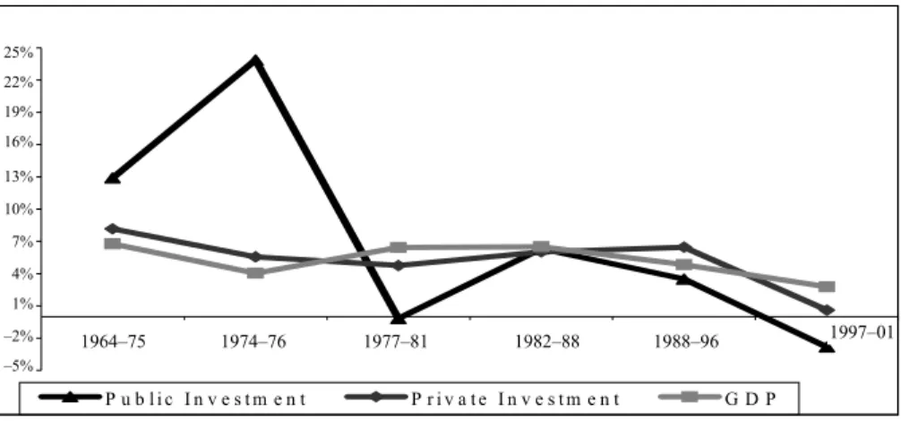
Average growth rates of GDP, public and private investment for different time periods beginning 1964 are shown in Table 1 and are plotted in Figure 1 below. The average growth rate of GDP and private investment are pro-cyclical for the periods 1964–73 and 1974–76. The average rate of growth of public investment shows an increasing trend for both these periods. The situation reverses when we compare the time-periods 1974–76 to 1977–81, as GDP and private investment become counter-cyclical with a decreasing trend in the public investment. From the period 1977–81 to 1982–88, average growth rates of GDP, public and private investment move ahead pro-cyclically. Average growth in public investment exhibits a declining trend in the 1982– 88 to 1988–96. During this period, the counter-cyclical behaviour of rate of growth of GDP and private investment is observed. For 1988–96 and 1997–2001, the growth rates of GDP, private and, public investment recorded pro-cyclical movements.
3Macro expenditure module, Macro-econometric model of SPDC.
4Although data for the earlier time-periods is available, we do not include it in our analysis to
Table 1
Trend of Public and Private Investment
Growth Rate (%) As a % of GDP Time Period Public Investment Private Investment GDP Public Investment Private Investment 1964–73 12.89 8.17 6.78 6.16 8.07 1974–76 23.87 5.55 4.04 11.67 7.37 1977–81 –0.18 4.74 6.43 11.12 8.12 1982–88 6.32 6.01 6.51 9.99 8.00 1988–96 3.48 6.45 4.83 8.75 8.22 1997–01 –2.83 0.60 2.77 6.05 8.34
The rising trend in public investment during 1964–1973 can be explained partly by the pro-industrial policies, especially in the import-competing sector. The policies of liberalisation and deregulation along with higher public investment resulted in higher level of GDP growth, public and private investment. Separation of Pakistan, oil price shocks, and the new economic agenda of the then new government changed the economic environment of the country during the time-period of 1973-76. New economic policies focused mainly on enhancing the size of public sector. The process of nationalisation, which started in mid 1970s, resulted in a massive enhancement in the public capital stock. Along with this, the economy experienced a level of relatively lower private investment and lower growth rate of GDP. Since 1977, the process of denationalisation, liberalisation and privatisation started. The main purpose of these policies was to boost private investment in the economy and to enhance economic development through market forces. These policies resulted in decline in the growth of public investment.
Fig. 1. Growth Rates. - 5 % - 2 % 1 % 4 % 7 % 1 0 % 1 3 % 1 6 % 1 9 % 2 2 % 2 5 % P u b l i c I n v e s t m e n t P r i v a t e I n v e s t m e n t G D P 25% 22% 19% 16% 13% 10% 7% 4% 1% –2% –5% 1964–75 1974–76 1977–81 1982–88 1988–96 1997–01
Rate of growth of GDP, public and private investment increased due to growth oriented strategies along with the policies of liberalisation and de-regulation during the 1982–88. Afterwards, in order to control the increasing budget deficit, the economic managers started reducing public sector development programme, which, however, increase the private investment due to the restoration of investor’s confidence in the early 1990s’. Finally, the policy of decreasing public investment resulted in lower private investment in the period of 1997–2001. The policy of gagging development expenditures resulted in lower economic growth and declining private investment. With this backdrop, it becomes essential to explore the optimal size of public expenditures. Presently, economic managers of Pakistan are following the policy of gagging development expenditures, which have resulted in lower overall economic growth also [Social Policy and Development Centre (2001)].
The above discussion summarises the average growth rate of GDP, public and private investment in specified time periods. The movements in the variables, however shows different relationships from the one time period to the other. Thus, there is need to analyse the behaviour of the growth of GDP, public and private investment in a dynamic framework.
The rest of the paper is organised as follows. In the second section, we review the existing empirical literature on crowding out hypothesis, especially with reference to Pakistan. The third section summarises and extends the model of Barth and Cordes (1980) in order to develop a theoretical framework for testing the crowding out hypothesis. It relates economic growth, public investment and private investments in the context of a neo-classical production function. In the fourth section, we review the multivariate time series techniques essential for estimating our model. The fifth section presents and discusses empirical results. Finally, in section six, major conclusions are outlined and policy recommendation and suggestions are provided for future research.
II. LITERATURE REVIEW
Many researchers have focused their attention towards examining the crowding out hypothesis in Pakistan. The test focuses on investigating the impact of change in public investment on private investment by analysing the impact of budget deficit on the interest rates. Some researchers [Ahmed (1994); Khan and Iqbal (1991)] come up with the conclusion that the crowding out phenomenon does not exist in Pakistan. Others support the crowding out hypothesis based on the finding of a positive association between interest rates and budget deficit.
Ahmed (1994) tests the crowding out hypothesis by estimating an IS-LM model for the period 1970-I to 1991-IV. The estimated equation relates the interest rate to real government spending, real budget deficit, real money stock, and the expected rate of inflation. He finds that none of the explanatory variables exert a significant influence on the nominal interest rate. The real interest rate is adversely
affected by the budget deficit due to the expected rate of inflation. From this evidence, he concludes no support for the crowding out hypothesis in the case of Pakistan. Khan and Iqbal (1991) also find no evidence in favour of the Keynesian (or conventional) crowding out hypothesis over the period 1959-60 to 1986-87. Burney and Yasmeen (1989) also study the impact of the budgetary links with interest rate for the period 1970-71 to 1988-89. Their finding shows no significant relationships between overall fiscal deficit and nominal interest rate. However, in an extreme case, when an assumption is made that people can predict the future rate of inflation accurately, the overall deficit is found to have a significant impact on the nominal rate of interest. These studies provide evidence against crowding out of private investment by the fiscal deficit, thereby implying that an increase in public investment may be desirable.
Some researchers [Kemal (1991); Khan (1988); Khan, Hasan and Malik (1992)] have debated against this testing procedure. They argue that the existence of financial repression (the term financial repression more commonly refers to interest rate ceilings), limits the robustness of the above studies. Khan (1988) and Khan, Hasan, and Malik (1992) identify the presence of financial repression in the capital markets of Pakistan by finding a positive and significant effect of the real interest rate on the national saving rate. They show that a one percent increase in the real interest rate is likely to increase the saving rate by 0.07 percent.
Looney (1995) utilises a modified Granger causality test to suggest that expanded public investment in infrastructure has not played an important role in stimulating private investment in the manufacturing sector of Pakistan. Granger causality test, however, provides limited information regarding the short run and long run relationship between the variables. Thus, a detailed time series analysis of the problem is required to have a better understanding of temporal and long run relationship among the variables. Haque and Montiel (1991, 1993) utilise their small scale macro-econometric model of Pakistan to conclude that the financing of budget deficits by non-bank borrowing results in an increase in public debt and hence crowds out private investment.
Two substantial observations can be made from the review of this literature. Firstly, that the researchers have focused on only one aspect of the crowding out phenomenon, that is the evaluation of the impact of budget deficit on interest rates. For concluding against crowding out, it is essential that we also corroborate the existence of a significant relationship between private investment and the rate of interest. This line of research currently remains unexplored and thereby imposes a limit on the usefulness of the results obtained earlier.5
5The Macroeconomic Expenditure block of SPDC macro-econometric model provides some
evidence on this issue. Separate regressions of investment in the agricultural, manufacturing and other sectors depict that only manufacturing sector investment (which is 27 percent of total investment) is weakly related to the nominal interest rate.
Secondly, the researchers have utilised the overall budget deficit to decide in favour of or against crowding out in Pakistan. In this connection, it must be explicated whether the overall budget deficit is a good variable to use in testing the crowding out phenomenon or not. Total fiscal deficit is the sum of two components. Public investment, and the deficit on government consumption. Whereas the latter is a pure burden on all current and future generations in terms of either taxes or public debt [Blanchard and Fisher (1995)], the former cannot be classified in the same way. In the case of developing countries where social overhead capital is inadequate, we can only classify public investment as a pure burden if the present value of its benefits does not exceed the present value of its provision and maintenance costs. This can only seldom be believed by any economist. Accordingly, a distinction must be made as to how we define the fiscal deficit variable to be included in such studies.
In this paper, we follow a slightly different methodology based on Barth and Cordes (1980) framework. Barth and Cordes (1980) study the crowding out phenomenon indirectly by analysing the impact of public sector capital formation and GDP growth on capital formation in the private sector. Their methodology, on the one hand, circumvents the first problem while on the other incorporates the second of the above criticisms to determine the existence or otherwise of crowding out in Pakistan. We develop the complete model in Section 3 below and review some econometric issues involved in its estimation in Section 4.
III. THEORATICAL FRAMEWORK
The interaction between public and private investment can be visualised in several different ways. Firstly, an increase in public investment in heavily subsidised and inefficient state-owned enterprises in various sectors more often reduces the possibilities for private investment and long run growth. Secondly, increase in public investment as a component of aggregate demand will increase economic growth. Furthermore, improvement in the economic and social infrastructure due to increased public spending will result in higher rate of return on private capital, which will ultimately encourage private investment. Thirdly, increase in private investment places pressure on the government to expand infrastructural facilities. The economic managers wishing to aid private investment while simultaneously lacking adequate funding for major infrastructural programmes may first grant the private sector various forms of relief such as tax holidays and exemptions followed by modest increase in public investment. This might result in higher budget deficits but not a crowding out of private investment.
The impact of public investment on capital formation in the private sector can possibly be analysed by using a modified neoclassical production function.6 A
neoclassical production function could then be written with separate arguments for public and private capital stocks:
Q = q(N, Kp, Kg) + ε … … … (1)
In the above equation, Q denotes the level of real output, N denotes
employment, Kpdenotes the stock of private capital and Kg refers to the public capital
stock. ε denotes a shift parameter of the production function which may account for Solow-type technical change as well as any other irregularities in the production process.
With this specification, it is possible to analyse the interaction between private and public capital formation and their impact on the level of output and employment. It provides an indirect means for examining crowding out by testing whether public and private capital stocks are substitutes or compliments to each other. If public and private capital stocks appear substitutes of each other, then an increase in the supply
of public capital would drive out private capital from production.7 If, however, they are complements in nature, then an increase in the public capital stock will reinforce an increase in the private capital stock by enhancing its productivity. Furthermore, the positive impact of increase in public capital stock on the marginal productivity of private capital stock and labour productivity will increase output. If both public and private capital stocks are weakly substitutable or weakly complementary, then an increase in public capital will only have a positive impact on output.
IV. ECONOMETRIC METHODOLOGY
The above specification only provides for the long run relationship between private and public capital stocks and aggregate output. The incorporation of short run dynamics in this behaviour can provide more information that is useful for predicting the future paths of these variables. Ghali (1998) utilises a dynamic version of the above framework to analyse the behaviour of the public and private investment in Tanzania. He makes use of multivariate time-series techniques to analyse the dynamic behaviour of public and private investment. Below we review some of these techniques.
7The Keynesian crowding out hypothesis is concerned with the demand rather than the supply
side of the economy. It simply predicts that if the demand for goods increases in the public sector then the demand for capital goods by the private sector will decline because of the increase in the interest rate. However, due to the unavailability of data on demand counterparts of the variables included in our model, we base our test on the supply variables instead. This is why we call our testing mechanism an indirect one. From a purely empirical standpoint, the difference between demand and supply is never visible, as observed data is always the equilibrium quantity traded in the market. Some researchers have suggested specifying an automated adjustment mechanism to convert supply data into demand data. This, undisputedly results in the inclusion of AR(1) variable in the final estimated equation. Our econometric methodology adequately takes into account this issue.
Consider the variables LYSR, LIPR, and LIGR, where LYSR denotes real GDP, LIPR denotes real private investment and LIGR denotes real public investment.8 If these variables are stochastically trending and if they have one common trend, then these variables should be co-integrated [Engle and Granger (1987)]. Co-integration is a test for equilibrium between non-stationary variables integrated of same order. According to the Engle and Granger (1987), co-integrated variable must have an error correction representation, or otherwise the regression would simply be based on spurious correlations.9
Let Xt be a vector containing the endogenous variables (LYSR, LIPR and
LIGR). Assume that these variables become I(0)after applying the difference filter
once. An exploitation of the idea that these variables exhibit co-movements and will trend together towards a long run equilibrium state enables us to posit the following testing relationships: t k t k t k t t t X X X X X =µ+ψ ∆ +ψ ∆ + +ψ ∆ +Π +η ∆ 1 −1 2 −2 LLL − − … … (2) This, according to the Granger representation theorem, constitutes a vector error-correction (VEC) model corresponding to Equation 1 above. ∆Xtis the vector of the growth rate of these variables, the ψ'sare estimable parameters,
∆
representsthe difference operator, ηt is an n.i.i.d~
( )
0,Σ vector of impulses which represent the unanticipated movements in Xt. ∑ represents the variance-covariance matrix ofthe impulses corresponding to each of the three variables. Π denotes the matrix of long run parameter of the model. With r co-integrating vectors
(
1≤r≥3)
,Π
has arank r and can be decomposed asΠ=αβ, with α and β both 3 x r matrices. β is a
matrix of the parameters in the co-integrating relationships and α are the adjustment coefficients which measure the strength of the co-integrating vectors in the VEC model. The Johansen (1988, 1992) and Johansen and Juselius (1990) multivariate co-integration techniques allow us to estimate the long run or co-integrating relationships between the non-stationary variables using a maximum likelihood procedure which tests for the co-integrating rank r and estimates the parameters β of
these co-integrating relationships. As proved by Johansen (1991, 1992), the intercept terms in the VEC model should be associated with the existence of a deterministic linear time trend in the data. If, however, the data do not contain a time trend, the VEC model should include a restricted intercept term associated with the co-integrating vectors.
The novelty of the co-integration approach is that empirical modeling of growth is not restricted to a particular functional relationship concerning the
8The data used in the study is collected from the various issues of
Economic Survey and Fifty Years of Pakistan.
variables’ behaviour. Rather, the approach is to let the data suggest the type of relationships that variables have in the long run. The co-integration methodology illustrates well the conflict that exists between the equilibrium framework and the disequilibrium environment from which the data are collected. As formulated by the VEC model, this conflict can easily be resolved by extending the equilibrium framework into one that accounts for disequilibrium by including the adjustment mechanisms represented by the error correction terms. Once the equilibrium conditions are imposed, the VEC model describes how the system is adjusting in each time-period towards its long-run equilibrium state. Since the variables are supposed to be co-integrated, then in the short term deviations from this long-run equilibrium will feed back on the changes in the dependent variables in order to force their movements towards the long-run equilibrium. Hence, the co-integrating vectors from which the error correction terms are derived are each indicating an independent direction where a stable, meaningful long-run equilibrium state exists. The coefficients of the error-correction terms, however, represent the proportion by which the long-run disequilibrium (or imbalance) in the dependent variables arc corrected in each short-term period.
Granger Causality
The co-integration methodology pioneered by Granger (1986); Hendry (1986) and Engle and Granger (1987) opened a new channel towards testing for Granger-causality. As Granger (1986, 1988) pointed out, if two variables are co-integrated then Granger-causality must exist in at least one direction. This result is a consequence of the relationships described by the error-correction model. Since the variables share common trends, then either ∆LYSR, ∆LIPR and ∆LIGRor a
combination of any of them must be Granger-caused by lagged values of the error-correction terms, which themselves are functions of the lagged values of the level variables. Intuitively, if LYSR t–p, LIPR t–p, LIGR t–p, share common trends, then the
current change, say ∆LYSR, is partly the result of LYSR moving in alignment with the
trend values of LIPR and LIGR. Given this, the temporal Granger-causality between
the variables can be investigated through the statistical significance of the lagged error-correction terms by applying separate t-tests on the coefficients of each of
them, and joint F-test or Wald χ2 test be applied to the coefficients of each
explanatory variable.
Impulse Response Analysis
Impulse response function describes the dynamic properties of the model following certain shocks. The impulse response function essentially traces out the moving average representation of the system and describes how one variable
responds to a single surprise increase in itself or in any other variable over a number of time-periods. For impulse response function, it is necessary that innovations of the system should be contemporaneously uncorrelated [Enders (1995)].
V. EMPIRICAL RESULTS Test Results for Unit Roots in the Data, 1964–2001
The tests used to investigate the existence of unit roots in the level variables as well as in their first differences are the Augmented Dickey-Fuller (ADF) and the Phillips-Perron (P-P) tests [Dickey and Fuller (1976, 1979), Phillips and Perron (1988)]. The test is performed on the level variables as well as on their first differences. The null hypothesis is that the variable under investigation has a unit root, against the alternative it does not. In each case, the lag length is chosen by minimising the Final Prediction Error (FPE) criteria due to Akiake (1969). We also test for the existence of up to the tenth order serial correlation in the residual of each regression using the Ljung-Box Q10 statistics.
The tests for unit roots are performed sequentially. As shown in Table 2 the variables at log level contain unit roots. Unit root is also tested for by assuming deterministic time trend, however, the null hypothesis that the level variables contain unit roots cannot be rejected by both the tests. Tests performed after differencing the series reject the null hypothesis of unit root. Since the data appear to be stationary in first differences, no further tests are performed.
The results of Table 2 are consistent with the null hypothesis that the level variables are each integrated of order one.
Table 2
Results of Stationarity Test
Stationarity Around a Non-zero Mean
Stationarity Around a Linear Trend
ADF P-P ADF P-P Log Levels LIPR –1.39 –1.63 –1.11 –2.96
LIGR –2.23 2.24 –0.85 –1.03
LYSR –2.45 –2.80 0.54 0.09
First Difference LIPR –3.53 –7.79
LIGR –3.01 –5.64
LYSR –3.36 –5.89
Critical Values 95% –2.94 2.94 –3.54 –3.54
10Ljung-Box Q statistics are 8.14, 3.43, and 5.62 for the regressions of LYSR, LIPR, and LIGR
Test Results of Co-integration
Before applying the Johansen’s procedure to α and β, it is necessary to determine the lag length, k, of the VAR, Equation (2), which should be high enough
to ensure that the errors are approximately white noise, but small enough to allow estimation. Since the Johansen procedure is sensitive to the choice of the lag length, we based our decision on the Akiake’s Final Prediction Error (FPE) criterion and selected k=5. Table 3 reports the diagnostic tests for normality and serial correlation
in residuals for each of the three equations in the VAR using k=5. This lag length left
the residuals approximately independently identically normally distributed for all the equations.
Table 3
Residual Diagnostic Tests for the VAR Equation k=5
LYSR LIPR LIGR
Normality Test Jarque-Bera 0.11 0.06 0.37
Probability 0.95 0.97 0.83
Serial Correlation Test Q-Statistic 7.99 4.83 8.60 The results for testing for the number of co-integrating vectors are reported in Table 4 which present both the maximum eigenvalue (λmax) and the trace statistics,
the 5 percent critical value as well as the corresponding λ values. This test is performed using an intercept term in the VAR model and assuming no deterministic trend. As can be noticed, both the λmaxand the trace statistics suggest the existence of
unique vector, which means the existence of two common stochastic trends. Table 4
Testing the Rank Π
Trace λmax
H0 H1 Stat. 95% 90% H0 H1 Stat. 95% 90% λ
r=0 r1 44.19 35.068 32.093 r=0 R=1 20.93 21.894 19.796 0.480 r1 r2 23.26 20.168 17.957 r1 R=2 17.38 15.752 13.781 0.419 r2 r3 5.87 9.094 7.563 r2 r=3 5.87 9.094 7.563 0.168
Since the specification of the deterministic components in the VEC model is essential for determining the method of estimation and, because the results above are obtained assuming the existence of unrestricted intercept term, we now check this assumption by testing the null hypothesis of the absence of a deterministic linear time trend in the data. To do this, we use the likelihood ratio test. The test result suggests no existence of deterministic trend.11
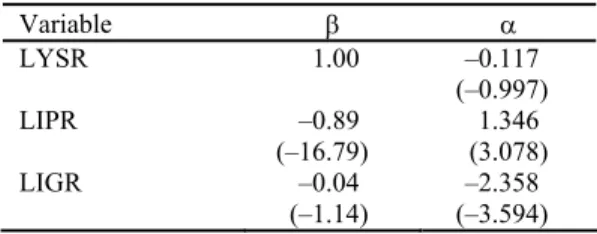
Table 5 αandβvectors Variable β α LYSR 1.00 –0.117 (–0.997) LIPR –0.89 1.346 (–16.79) (3.078) LIGR –0.04 –2.358 (–1.14) (–3.594) Table 6 Results of Co-integration
Variable ∆LYSR ∆LIPR ∆LIGR
Coint –0.117 1.346 –2.358 (–0.997) (3.078) (–3.594) ∆LYSR-1 0.292 1.563 1.730 (1.650) (2.362) (1.743) ∆LYSR-2 –0.287 –1.396 1.179 (–1.291) (–1.680) (0.945) ∆LYSR-3 0.322 0.433 0.582 (1.768) (0.637) (0.570) ∆LYSR-4 0.616 –0.631 3.260 (3.077) (–0.842) (2.902) ∆LYSR-5 0.069 –2.177 3.135 (0.313) (–2.657) (2.548) ∆LIPR-1 0.026 0.768 –2.162 (0.226) (1.807) (–3.390) ∆LIPR-2 0.021 0.471 –1.206 (0.227) (1.369) (–2.334) ∆LIPR-3 –0.071 –0.297 –0.686 (–0.998) (–1.120) (–1.728) ∆LIPR-4 0.053 0.204 –0.568 (0.915) (0.936) (–1.738) ∆LIPR-5 –0.008 –0.325 –0.368 (–0.163) (–1.731) (–1.305) ∆LIGR-1 0.009 0.318 –0.173 (0.185) (1.718) (–0.625) ∆LIGR-2 –0.038 –0.061 0.150 (–0.965) (–0.417) (0.688) ∆LIGR-3 –0.017 0.623 –0.228 (–0.376) (3.748) (–0.913) ∆LIGR-4 –0.117 –0.480 –0.033 (–2.494) (–2.735) (–0.124) ∆LIGR-5 0.196 0.239 –0.350 (4.083) (1.328) (–1.297) R-squared 0.754 0.770 0.654 F-statistic 3.271 3.573 2.016 Log Likelihood 98.826 56.613 43.625 N(2) 0.43 0.08 1.19 TSC(10) 8.65 3.91 5.67
The results above indicate that the variables are moving together towards a stable, long-run equilibrium state. The co-integrating vector indicates the direction where such equilibrium exists and the adjustment coefficients indicate the speed of adjustment of each variable to this long-run equilibrium. From the long-run relationships between the variables given by the co-integrating equation, we can see that in the long-run private and public investment has a positive impact on growth. Moreover, from the estimated α vector we can see that the speed of adjustment of private investment to the long-run equilibrium is higher than the speed of adjustment of public investment.
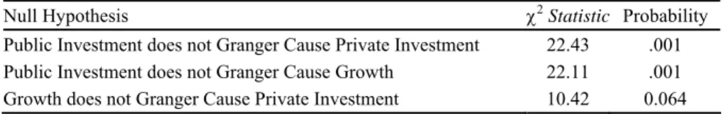
Results of the Granger causality are described in the Table 7, which suggest that public investment Granger-cause both the growth and private investment. While economic growth Granger cause private investment only. The results of the Granger causality are consistent as the causality exists in one direction that is from public investment to the growth and private investment and from growth to private investment.
Table 7
Granger Causality Test
Null Hypothesis χ2Statistic Probability
Public Investment does not Granger Cause Private Investment 22.43 .001 Public Investment does not Granger Cause Growth 22.11 .001 Growth does not Granger Cause Private Investment 10.42 0.064
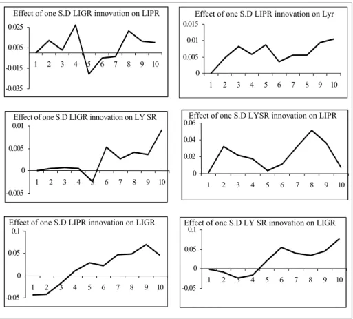
Impulse response functions are employed to investigate the effects of GDP, public and private investment. Since, all the three variables are endogenous in the error-correction model so the coefficients are not structural but derived from a reduced form system. These support the validity of the results of impulse response function (IRF).
Same order of variables is used in the IRF as in the estimation of co-integrating equation. This ordering is followed because of the sensitivity of the IRF to the ordering of variables. The IRF derived from the Error-correction model is presented in the Figure 2.
The figure indicates the response of one standard deviation shock in one variable on the other variables of the system. The shock in public investment results in an increase in the private investment in the initial periods of forecast and then after a declining for three periods it starts increasing. The impact on the GDP of one standard deviation shock in public investment is negligible in the first four periods and positive in the remaining periods. In a similar manner, shock in the private investment results in an increase in the public investment after three periods and an increase in GDP in all the forecast periods. A positive shock in GDP has a positive impact on public investment while private investment exhibits positive movement after four periods.
Fig. 2. Results of Impulse Response Function.
These results confirm the complementary relationship between public and private investment. GDP is also positively associated with both the category of investment. This provides clear evidence in support of “crowding in” hypotheses in
Pakistan.
VI. CONCLUSIONS AND POLICY RECOMMENDATIONS
In this paper we made an attempt to test the crowding out hypothesis in Pakistan using vector error-correction framework. We carried out the analysis using data on gross domestic product, public investment and private investment from 1964 to 2001. Standard Dickey-Fuller tests show that all these time series are non-stationary in levels and become non-stationary after applying the first difference operator. The Johansen test shows that they are also co-integrated of order one-one. As such,
0 0.005 0.01 0.015 1 2 3 4 5 6 7 8 9 10 -0.035 -0.015 0.005 0.025 1 2 3 4 5 6 7 8 9 10 -0.005 0 0.005 0.01 1 2 3 4 5 6 7 8 9 10 0 0.02 0.04 0.06 1 2 3 4 5 6 7 8 9 10 -0.05 0 0.05 0.1 1 2 3 4 5 6 7 8 9 10 -0.05 0 0.05 0.1 1 2 3 4 5 6 7 8 9 10
Effect of one S.D LIGR innovation on LIPR Effect of one S.D LIPR innovation on Lyr
Effect of one S.D LYSR innovation on LIPR Effect of one S.D LIGR innovation on LY SR
we estimate an error-correction model to study the dynamic interaction among the variables and apply the Granger causality test to explore the direction of causal relationships.
The results of the error correction model and impulse response analysis support a complementary relationship between public and private investment in Pakistan. Granger causality test shows that public investment has a significant impact on private investment while GDP growth significantly affects private investment. We also conducted impulse response analysis to forecast the time paths of the endogenous variables in the model. The orthogonality of the ECM residuals indicates that such analysis will be meaningful. The results of impulse response analysis substantiate the results of the ECM.
The rejection of crowding out hypothesis suggests that an increase in public investment would result in an increase in both private investment and GDP growth. Our analysis shows that the fiscal consolidation policy pursued by economic managers can only be defended if we willingly overlook this empirical finding. This policy stance implemented under the IMF stabilisation programme has lead to a retardation of growth in the economy. Our analysis implies that a policy of increasing public investment will boost economic growth and private investment in the economy.
REFERENCES
Abel, A. B., and B. S. Bernanke (1992) Macroeconomics. Reading, Mass, Don Mills
Ont Wokingham, U. K. and Sydney: Addison Wesley.
Ahmed, M. (1994) The Effects of Government Budget Deficits on the Interest Rates: A Case Study of a Small Open Economy. Economia Internazionale 1, 1–6.
Aisha, A. F., and H. A. Pasha (2000) Macroeconomic Framework for Debt Management. Social Policy and Development Centre. (Policy Paper No. 19.)
Akiake, H. (1969) Fitting Autoregressive Models for Prediction. Annals of International Statistics and Mathematics 21, 243–47.
Aschauer, D. A. (1988) Government Spending and the Falling Rate of Profit.
Economic Perspectives 6, 11–17.
Barth, J. R., and J. J. Cordes (1980) Substitutability, Complementarity, and the Impact of Government Spending on Economic Activity. Journal of Economic and Business 2, 235–42.
Blanchard, O., and S. Fischer (1994) Macroeconomic Dynamics. Cambridge: MIT Press.
Burney, N. A., and A. Yasmeen (1989) Government Budget Deficit and Interest Rates: An Empirical Analysis of Pakistan. The Pakistan Development Review
28:4, 971–80.
Dickey, D. A., and W. A. Fuller (1979) Distribution of the Estimators for Autoregressive Time Series with a Unit Root. Journal of American Statistical Association 75, 427–831.
Dickey, D. A., and W. A. Fuller (1981) Likelihood Ratio Statistics for Autoregressive Time Series with a Unit Root. Econometrica 49, 1057–72.
Enders, W. (1995) Applied Econometric Time Series. John Wiley & Sons, INC.
Engle, R. E., and C. W. J. Granger (1987) Cointegration and Error Correction: Representation, Estimation and Testing. Econometrica 55, 251–76.
Ghali, K. H. (1998) Public Investment and Private Capital Formation in a Vector Error-correction Model of Growth. Applied Economics 6, 837–44.
Granger, C. W. J. (1986) Development in the Study of Cointegrated Economic Variables. Oxford Bulletin of Economics and Statistics 48, 213–28.
Granger, C. W. J. (1988) Some Recent Developments in the Concept of Causality.
Journal of Econometrics 39, 199–211.
Haque, N. U., and P. J. Montiel (1993) Fiscal Adjustment in Pakistan: Some Simulation Results. International Monetary Fund Staff Papers 40:2, 471–80.
Hendry, D. F. (1986) Econometric Modelling with Cointegrated Variables: An Overview. Oxford Bulletin of Economics and Statistics 48:3, 201–12.
Jarque, C. M., and A. K. Bera (1980) Efficient Test for Normality, Heteroscedasticity and Serial Independence of Regression Residuals. Economic Letters 6, 255–59.
Johansen, S. (1988) Statistical Analysis of Cointegration Vectors. Journal of Economic Dynamics and Control 12, 231–54.
Johansen, S. (1991) Estimation and Hypothesis Testing of Cointegration Vectors in Gaussian Vector Autoregressive Models. Econometrica 59, 1551–80.
Johansen, S. (1992) Determination of Cointegrating Rank in the Presence of a Linear Trend. Oxford Bulletin of Economics and Statistics 54, 383–97.
Johansen, S., and K. Juselius (1990) Maximum Likelihood Estimation and Inference on Cointegration with Applications to the Demand for Money. Oxford Bulletin of Economics and Statistics 52, 169–210.
Kemal, A. R. (1991) Options for Financing the Budgetary Deficit, Money Supply, and Growth of Banking Sector. The Pakistan Development Review 30:4, 769–81.
Khan, A H., Lubna Hassan, and A. Malik (1992) Dependency Ratio, Foreign Capital Inflows and the Rate of Saving in Pakistan. The Pakistan Development Review
31:4, 843–56.
Khan, A. H. (1988) Financial Repression, Financial Development and Structure of Saving in Pakistan. The Pakistan Development Review 27:4, 701–11.
Khan, A. H. (1988a) Macroeconomic Policy and Private Investment in Pakistan. The Pakistan Development Review 27:3, 277–91.
Khan, A. H., and Z. Iqbal (1991) Fiscal Deficit and Private Sector Activities in Pakistan. Economia Internazionale 2-3, 182–90.
Looney, R. E. (1995) Public Sector Deficits and Private Investment: A Test of the Crowding-Out Hypothesis in Pakistan’s Manufacturing Industry. The Pakistan Development Review 34:3, 277–97.
Looney, R. E., and P. C. Frederiken (1997) Government Investment and Follow-on Private Sector Investment in Pakistan, 1972-1995. Journal of Economic Development 22:1, 91–100.
Monadjemi M. S. (1996) Public Expenditure and Private Investment: A Study of Three OECD Countries. (University of Kent Working Paper Series.)
Pakistan, Government of (Various Issues) Economic Survey. Islamabad: Economic
Advisor’s Wing, Ministry of Finance.
Pakistan, Government of (Various Issues) Fifty Years of Pakistan. Islamabad:
Federal Bureau of Statistics.
Pakistan, Government of (Various Issues) National Income Accounts. Islamabad:
Federal Bureau of Statistics.
Pasha, H. A., and A. F. Aisha (1996) Growth of Public Debt and Debt Servicing in Pakistan. Social Policy and Development Centre. (Research Report No. 17.) Ramirez, M. D. (1994) Public and Private Investment in Mexico 1950–90: An
Empirical Analysis. Southern Economic Journal 61, 1–17.
Social Policy and Development Centre (2001) Stabilisation Versus Growth. (Research Report No. 40.)
Comments
It is my pleasure to comment on Mr Kalim Haider’s very good paper on the empirical analysis of the crowding-out hypothesis.
On testing the crowding-out hypothesis the paper uses rigorous methodology comprising unit roots, cointegration, and error correction mechanism. The results and conclusions of the paper are important in the context of Pakistan economy. The author picks three variables, that is, GDP, public investment, and private investment and investigates the presence of any causal relationship among the variables. The prime objective, I suppose, of the study is to find the appropriate variable from public and private investment that could be used as a policy variable to enhance growth.
I have some serious observation on the results of the study, through.
(1) In Table 5, the author presents cointegrating vector (β) and loading vector (α) and claims that there is a positive relationship between the public and private investment and growth. There is no evidence in the paper that author has tested the significance of individual parameter. If the figures in the parentheses are test statistics for significance, then the public investment has no long-run relationship with GDP.
(2) Further, Table 6 shows that it is a result of cointegration analysis. I suppose it is the error correction model that should have been used for causality analysis. The results indicate that the error correction term is significant in the second and third equation. It can be interpreted that there is causal relationship between the variables and the causality runs both ways. I suggest the author should re-evaluate and reinterpret the results by considering what is presented in the Tables.
(3) Finally, I think that most of the conclusions presented in the paper are based on the Table 7. Apparently this table has no relationship with the methodology specified in the earlier part of the paper and claimed to be used by the author for analysis in this paper. This Table is an output from the econometric package. It is a result of simple Granger causality test. It is not a test of causality that is proposed by Engle and Granger (1987). I would like author to clarify the results.
Abdul Qayyum
Pakistan Institute of Development Economics, Islamabad.