Context-Aware Deep Sequence Learning with Multi-View Factor Pooling for Time Series Classification

Context-Aware Deep Sequence Learning with Multi-View Factor Pooling for Time

Series Classification

Sreyasee Das Bhattacharjee, William J. Tolone, Mohammed Elshambakey, Isaac Cho College of Computing and Informatics University of North Carolina at Charlotte

Charlotte, United States

Ashish Mahabal, George Djorgovski Department of Astronomy California Institute of Technology

Pasedona, United Sates

Abstract—In this paper, we propose an effective, multi-view, multivariate deep classification model for time-series data. Multi-view methods show promise in their ability to learn correlation and exclusivity properties across different independent information resources. However, most current multi-view integration schemes employ only a linear model and, therefore, do not extensively utilize the relationships observed across different view-specific representations. Moreover, the majority of these methods rely exclusively on sophisticated, handcrafted features to capture local data patterns and, thus, depend heavily on large collections of labeled data. The multi-view, multivariate deep classification model for time-series data proposed in this paper makes important contributions to address these limitations. The proposed model derives a LSTM-based, deep feature descriptor to model both the view-specific data characteristics and cross-view interaction in an integrated deep architecture while driving the learning phase in a data-driven manner. The proposed model employs a compact context descriptor to exploit view-specific affinity information to design a more insightful context representation. Finally, the model uses a multi-view factor-pooling scheme for a context-driven attention learning strategy to weigh the most relevant feature dimensions while eliminating noise from the resulting fused descriptor. As shown by experiments, compared to the existing multi-view methods, the proposed multi-view deep se-quential learning approach improves classification performance by roughly 4% in the UCI multi-view activity recognition dataset, while also showing significantly robust generalized representation capacity against its single-view counterparts, in classifying several large-scale multi-view light curve collections.

Keywords-LSTM, RNN, Multi-view Classification, Deep Learning, Time-Series Data, Bilinear Pooling, Matrix Factor-ization

I. INTRODUCTION

In this paper, we propose an effective, multi-view, mul-tivariate deep classification model for time-series data that monitors and investigates continuously streaming object in-formation collected via multiple independent views to learn complex, latent data patterns. Multi-view time-series data are prevalent in many fields including finance, medicine, secu-rity, surveillance, and astronomy. Integration of information across different views is critical to model the exhaustive object characteristics within an integrated, deep learning

framework that can efficiently and effectively identify com-plex patterns within multi-view time-series data. However, while integration can happen at different stages, efficiency and scalability of the integration scheme are also some of the most critical challenges in many application settings. More-over, in most cases, multi-view integration schemes simply employ a linear model and, therefore, do not extensively utilize the relationships observed across different view-specific representations [1], [2]. In fact, since multi-view feature distributions commonly vary quite significantly, such linear models often are not sufficiently expressive to obtain a comprehensive derived representation that can capture the complex association patterns with sufficient reliability. The multi-view framework designed in this work, aggregates information from three complementary resources to show a promising enhancement in the resulting classification per-formance, compared to its single-view counterparts.

Several specialized metrics like Dynamic Time Wrapping (DTW) [3], edit distance [4], elastic distance [5] or several others, e.g., [6], have been proposed to overcome specific challenges associated with time-series classification. How-ever, the basic assumption in most of the existing literature is the availability of a large collection of labeled data samples in a single-view environment. In fact, a majority of these methods rely exclusively on extracting sophisticated, hand-crafted features to capture the local data patterns. Therefore, the efficiency and precision of these classification approaches are heavily dependent on the availability of large collections of labeled data that capture the entire spectrum of data characteristics and the quality of the hand-crafted features used to define a comprehensive descriptor. Multi-view methods have shown promise in their ability to learn correlation and exclusivity properties across different inde-pendent information resources, by enabling methods like co-training, specialized kernel learning, and subspace learning [7], [8]. However, extensions to these existing approaches to handle time-series data are nontrivial.

The multi-view, multivariate deep classification model for time-series data proposed in this paper makes important steps to address these limitations. A small set of statistical

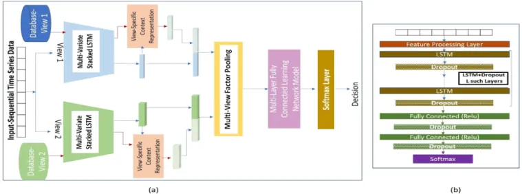
Figure 1. (a) The Proposed Multi-View Deep Learning Framework. (b) Architecture of a single-view classifier, where the output from theLth _layer, forms the view-specific representative of the input signal.

features (e.g., mean, min, max, media, skew, kurtosis) as well as specialized domain knowledge (e.g., ‘fading profile of a single peaked fast transient’) are used to construct a multivariate deep classification model for multi-view time-series data (e.g., light curves generated from multiple views), which has also shown reasonable effectiveness in handling missing view information (e.g., missing view information of the underlying originating resource of the light curve). The proposed method uses a stacked LSTM model to derive a deep feature descriptor representing the sequential data input streaming into the system. In order to learn more exhaustive insight on the characteristics of the input sequence, the pro-posed compact context descriptor exploits its view-specific affinity information within the existing data repository to design a more insightful context representative.

While binary pooling [9] has been effective to fuse different CNN features [10], the high-dimensional of the resulting output and a large number of system parameters may seriously hinder the applicability of binary pooling in a practical problem setting. To address these issues, the proposed multi-view factor pooling scheme adopts a context-driven attention learning strategy to weigh the most relevant feature dimensions while eliminating the noises within the resulting fused descriptor.

The primary contributions reorted in this paper can be summarized as follows: 1) the proposed multi-view fac-tor pooling scheme incorporates the complementary view-information within an integrated attention learning frame-work to ensure a robust expressive capacity; 2) the proposed deep learning module is designed to execute the entire learning during multiple phases in a distributive manner, which makes the process more flexible and easily adoptable in various practical application settings, and, 3) a view-specific context representation scheme enables a dynamic

adaptation of the proximity information within the existing database to offer a more powerful representation for the multi-view sequence data.

The rest of the paper is organized as follows: Section II briefly describes the related works. Section III describes the proposed method. Section IV and Section V represent the experimental results and concluding thoughts respectively.

II. RELATEDWORKS

In this section, we briefly describe relevant research related to our work on multi-view, deep, sequence classi-fication, including bilinear attention learning, multivariate time-series classification, and multi-view learning.

Multivariate representation of time-series data is recently a popular method for solving classification tasks such as: (1) developing customized metrics that offer more insight-ful similarity measures; (2) constructing specialized classi-fiers; and, (3) developing feature-based methods. Typically, distance-based methods design metrics by considering the temporal dynamics and the probable misalignment between these dynamics. One such metric is the widely used Dy-namic Time-Warping (DTW) method [3], which has been used successfully to classify multivariate time-series data [11]. In fact, research indicates that DTW is an effective distance-based measure, along with nearest neighbor clas-sifiers. On the other hand, a common strategy leveraged in feature-based methods is to apply rigid dimension reduction techniques such as Principal Component Analysis (PCA) to obtain a univariate derived signal [12] representation. However, learning a large number of latent variables, which increases linearly with the number of model parameters, makes the process both computationally expensive and prone to overfitting. The objective of these methods is to extract a set of discriminative features, which are then used as input to

model the classifiers. A detailed discussion of such represen-tations schemes can be found in [13]. Unfortunately, many of the existing approaches are based on handcrafted feature engineering that require intensive preprocessing based on expert insights, an approach that is insufficiently general.

In contract to these shallow, feature-based learning mod-els, other approaches attempt to apply deep learning-based techniques to the problem of time-series data classification [14]. Yi ei al. [14] have proposed using Multi-channel Deep Convolutional Neural Network (MC-DCNN) for mul-tivariate time-series classification, wherein, input from each variable is used to obtain latent features, which are then fed in a Multi-Layer Perceptron (MLP) to perform clas-sification. Karim et al. [15] augment existing LSTM-FCN and ALSTM-FCN with a squeeze and excitation block for an improved performance. A detailed review of these approaches can be found in [16]. However, extending these existing works to handle multivariate data originated from distributed multi-view environment is nontrivial.

In this work we address the challenge of multivari-ate, time-series classification using a multi-view approach, which in a distributed environment can model nonlinear context information on the fly within an attention learning framework for a more insightful representation scheme. The proposed multi-stage deep learning-based classification approach leverages time-series data from multiple views, possibly with missing view details, to allow for greater flexibility in practical application settings. While multi-view learning is widely applicable for problems like classification [17] and outlier detection [18], there are few results that include temporal information in the multi-view setting. To incorporate temporal information, we apply matrix factor-ization to combine multi-view representations in a general, context-driven attention learning framework to obtain a compact multi-view representation that is proven to be more discriminative for improved classification performance.

III. PROPOSEDMETHOD

A multivariate series representation of a set of time-series signals {xi}i is defined in terms of an ordered sequence fi = {fi,1,·,·,·, fi,T} of T time steps, where each fi,j = (fi,j1 ,·,·, fi,jd ) ∈ Rd is represented using the

jth _{time step response of d(∈}

N)-streams. For example, the streams of dstatistical features represent the same light curve signal atT time steps. In our multi-view framework, Dv={(xvi, cvi)}irepresents the annotated sample collection available for view v ∈ V, where cv

i ∈ {1, ...c} is the label for the signalxv_i1_{, represented byf}v

i.

Given the entire collection of annotated samples D = ∪v∈VDv, the task is to learn an effective multi-view model

1_{Please note that for different views, the dimensiondoff}

i,j can differ and therefore the dimension of fv

i representing xvi can vary. However, for simplicity and without loss of generality, we holddconsistent across different views in this presentation.

for classifying an incoming signalx. It is important to note that, in some cases, x may also have some missing view information. In fact, the representation ofxmay be available only for some views in V, but not all. Long Short-Term Memory (LSTM) network model, a variant of Recurrent Network Model (RNN), is adopted for obtaining the time-series descriptor, the details of which are described briefly below.

A. Long Short-Term Memory (LSTM)

Recurrent Neural Networks (RNN) are a form of neural networks that display temporal behavior through the direct connections between individual layers. Given xi and its

d-dimensional temporal representative sequence fi, in an iterative learning phase, RNNs are designed to propagate historical information via a chain-like neural network archi-tecture that simultaneously takes into consideration of the current input fi,t at tth iteration, and well as the hidden stateh(_it−1) at each time step [19].

However, standard RNNs face a vanishing gradient prob-lem and are unable to learn long-term dependencies as the time steps become large. To address this challenge, Long Short-Term Memory (LSTM) has emerged as an efficient alternative that integrates the gating functions into its state dynamics [20]. In this work, stacked LSTM models are used as the feature extraction modules to obtain view specific representations of the multi-view, deep learning networks. In a stacked LSTM withLlayers, the final hidden layerL,

h(_it)=h(_L,it), which depends on the input sequence and cell state, defined as follows:

h(_l,it) = o_l,i(t)tanh(c(_l,it)) c_l,i(t) = r(_l,it)c_l,i(t−1)+j(_l,it)g(_l,it) g(_l,it) = tanh Ig_lh_l(₋t)_1,i+Wg_lh(_l,it)

r(_l,it) = σ Ir_lh_l(₋t)_1,i+Wr_lh(_l,it) j(_l,it) = σ Ij_lh_l(₋t)_1,i+Wj_lh(_l,it)

(1)

o(_l,it) = σ Io_lh_l(₋t)_1,i+Wo_lh(_l,it)

where h(₀t_,i) = fi,t, σ() represents the logistic sigmoid function, andrepresents the element wise multiplication. The termsc(0)_l,i,h(0)_l,i are set to zero vectors for all1≤l≤L. The termg(_l,it)is a hidden representative based on the current input and the previous state. The terms r(_l,it), j_l,i(t), and o(_l,it)

determine the cell information flow with time, how the input is incorporated into the cell state, and the relation between hidden state and the cell state, respectively. The recurrent learnable weights are depicted byWg,Wr,Wj, andWo

and the projection matrices byIg,Ir,Ij andIo.

An overview of the proposed multi-view deep learning architecture is illustrated (for a 2-view setting) in Figure

1(a), in which the first set of components is its |V| mul-tivariate stacked LSTM sequence representation modules {Sv}v∈V, each representing the data patterns learned from

the annotated sample collection in Dv, for v ∈ V. Figure 1(b) shows the single view architecture. Given xi ∈ Dv, the last hidden vector of the learned view-specific stacked LSTM modelSv at layerL, denoted ashvi ∈Rm, is treated as thev view representative ofxi.

B. Context-Aware View Representation

In order to gain more contextual insight of the view-specific characteristics of a sample x(represented by its v

view representativehv learned fromSv),N

{K,v}

i , the set of itsK-nearest training samples inDvare aggregated by sum-pooling to derive a compact v-view context representative

nv_{. In other words, givenxandN}{K,v}

i ={x

v

n}Kn=1, which

is a subset ofDv,nv is defined as:

nv[p] = K X n=1 hv_n[p] ∀p∈ {1,2,·,·, m} (2) where, hv

n is the view representation of xvn. In all our experiments, we have usedK= 10andnv_isl

2normalized

(z→ z

||z||) to represent thev view-specific context for x.

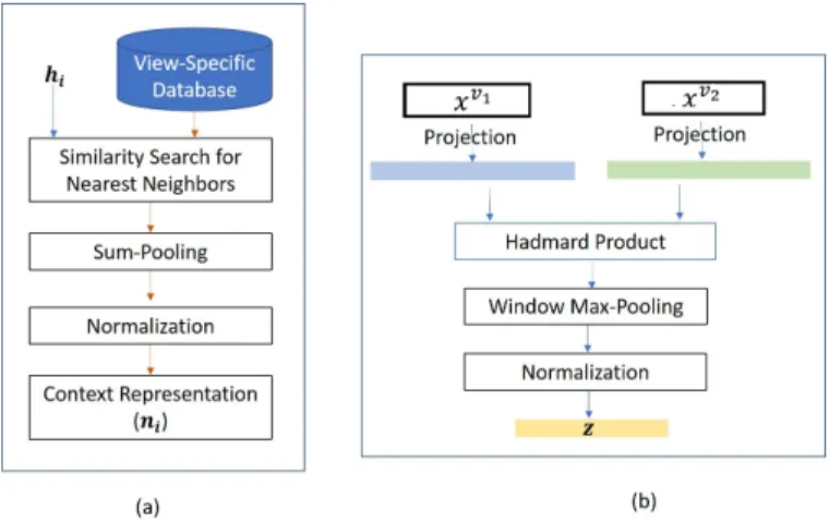
The entire context representation mechanism is illustrated in Figure 2(a). Given x, hv _{and n}v _{are combined with} operator C(., .), such that yv _{= C(h}v_,nv_{) is used as the}

v-view representative of x learned from Sv. In this work, we assume C(., .) to be the concatenation of the feature maps in depth to obtainyv _∈

R2mas a context-aware view representative, although other choices are possible.

C. Multi-View Factor Pooling

An insightful view invariant feature representative, which can capture all relevant information regarding its likely char-acteristics across multiple views in consideration and also allows for flexibility in handling different feature descriptor sizes for different views, is obtained by designing bilinear factor pooling.

Given a signal x, two feature vectors fv1 ∈

Rd1×T _and

fv2 ∈

Rd2×T_{, representing its two different views, the}

multi-view interaction model is inspired by the matrix factorization technique proposed for uni-modal data [21]. Without loss of generality, fv1 _{and f}v2 _{can respectively be reshaped to}

form a 1-D vector f0v1 _∈

Rd1T×1 _{and f}0v2 _∈

Rd2T×1_{. To}

obtain a reduced d0 dimensional multi-view representative

z, the view-specific learned weights are represented in terms of two order-three tensors U = [U1,·,·, Ud0] ∈ R

d1×T×d0

andV= [V1,·,·, Vd0]∈R

d2×T×d0_{, which are respectively}

reshaped to derive two dimensional transformed matrices

U0 ∈Rd1T×d0 _andV0 _∈

Rd2T×d0_{. The interaction is then}

defined as :

z = (f0v1₎T_U0_V0T_f0v2 ₍₃₎

= Sum{U0Tf0v1_V0T_f0v2_}

Figure 2. (a) The proposed view-specific context representation scheme. (b) Multi-view Factor Pooling.

whereSum{v}computes the sum of the elements ofvand

d0 is the latent dimensionality of the factorization matrices

U0 and V0. The operator is the Hadmard product. In a two-view setting, considering d0 = m, Eqn. (2) can be

rewritten as: nvi_{[p] =} K X n=1 U0Tf_n0vi_{[p]∀i∈ {1,2} andp∈ {1,·,·, m}}

and Eqn. (3) is then modified as:

z=SumP ool

C(U0Tf0v1_,nv1_{) C(U}0T_f0v2_,nv2_{), w}

(4)

which uses a non-overlapping window of size w to per-form the sumpooling. In all our experiments, we consider

w = 2 to achieve a d0 dimensional vector z, which is

then l2 normalized to obtain the multi-view representative

of x. Thus, by combining the multiple context-rich, view-specific feature representatives within a compact descriptor, the proposed sequence representation module is enabled to implicitly capture cross-view attentions effectively. This process of Multi-View Factor Pooling (MVFL) is illustrated in Figure 2(b).

D. Deep Classification Module

The output of the MVFL is fed into a stack of Fully Con-nected (FC) layers for classification. The proposed model uses 2 layers of FC layers. While adding more layers makes the network more expressive, it at the same time becomes harder to train due to increased computation time complex-ity, vanishing gradients, and model overfitting. In order to address the issue of overfitting, dropput based regularization is employed, which randomly chooses a percentage κ of hidden units during the forward backpropagation step. This is used to cancel the contribution of some randomly chosen weight vectors in the network. A scaled version of the learned weight (wsc=κ·w) without applying the dropout,

is used at the inference step. The standard back propagation algorithm is employed to update FC layer weight parameters in Wf_{. More specifically, if F denotes the loss function} defined as follows: F(Wf) =− P l∈{0,1} P|D| i=1N{ci=c}logp(ci=c|xi;Wf) |D| (5) where N{.} is the indicator function, Wf represents the CNN weight parameters, and prob(ci = c|xi;Wf) com-putes the probabilistic score of the samplexifor the classc. The task is formulated as solving the minimization problem defined as:min

Wf F(W

f_{). The activation of the last FC layer} is fed into a softmax layer to obtain the probabilistic class membership scores.

IV. EXPERIMENTS

A. Dataset

In this section, the performance of the proposed method is evaluated by analyzing the results of several experiments conducted for two types of classification tasks: (1) Light Curve Classification, and (2) Daily Activity Recognition. These specific choices for testbeds are influenced by their unique application specific challenges, which make the cor-responding classification task more complex.

In the first set of experiments, to accurately classify multiple large periodic light curve collections [22], one of the major challenges is the variance in the measurements frequently observed for similar light curves obtained from different telescopes. In this dataset, the goal is to achieve a classifier that can learn a robust feature representation scheme, which is sufficiently view-invariant. In this work, the first collection of light curves is taken from Catalina Real-Time Transient Survey (CRTS), which spans 33,000 sq. degrees encompassing light curves of close to half a billion sources. A set of ∼ 50k periodic variables from CRTS North (CRTS-N) survey builds one single view sub-collection of D. The other view-specific sub-collections of D include ∼37k samples from CRTS-South [23], ∼ 15k

samples from Palomar Transient Factory (PTF) [24], and ∼ 17k samples from the 2018 Gaia data release-2 [25]. PTF survey has used a more mixed cadence with a greater emphasis on looking for explosive events including a repeat cadence of 1, 3, 5 nights. In our experiments, PTF data with ‘r’ filter are chosen. The fourth collection, Gaia Data Release2 (DR2) contains celestial positions and the apparent brightness in ‘G’ for approximately 1.7 billion sources. The sample of sources for which variability information is provided is expanded to 0.5 million stars. The instrument captures images at three different bands: white-light ‘G’; Blue Prism (‘BP’); and Red Prism (‘RP’). A separate set of multi-view experiments with this dataset uses subsets of each of these samples as a single view data collection and, thus, the entire multi-view collection D contains the Gaia

DR2 data at all three different bands. CRTS-N contains samples from 17 classes in the entire sample collection. Any class with fewer than 500 samples is added entirely to the training collection. The present collection of CRTS-N data contains 10 of such classes. In contrast to excluding these samples completely from the experimental settings, by adding them within the training collection we aim to create a more challenging multi-class learning environment for the system. This also ensures the learning of an effective model capable of classifying future samples from those classes for which number of samples were less in the present version of the data release, without needing for a complete system update. CRTS-S uses the same asteroid-finding cadence as CRTS-N and also has an open filter. The same set of classes for which both CRTS-N and CRTS-S has sufficient samples for testing, are used to build the CRTS-S test collection. The released PTF and Gaia DR2 collection have 5 and 6 such classes, respectively, with at least500representative samples to constitute their training collection.

The second dataset used in this work is the UCI Daily and Sports Activity Dataset [26], which contains motion sensor data of 19 daily and sports activities (listed as A1, ..A19) such as sitting, standing, walking, running, jumping, etc. Each activity is performed by 8 subjects (4 males and 4 females) within the age range [20,30] for 5 minutes. The subjects were asked to perform the activities freely in their own styles, which resulted in a considerable intraclass variations observed within each activity type in terms of speed and amplitude, which creates additional challenge for precise classification. Nine sensors are placed at each of 5 different units: torso, right arm, left arm, right leg, and left leg, providing45 sensors in total. Each sensor is calibrated to acquire data at a 25 Hz sampling frequency. The 5-minute time-series collected from each subject is divided into 5-second segments. Therefore, each segment has in total 125 samples, from which 50 random samples are chosen to define a single database segment. While there are 125₅₀ such choices, we select 20 of them to build a suffciently large representative samples per activity. Samples from similar activities like standing and standing in an elevator are treated to describe the same activity class. Therefore, the dataset has11classes:Sitting(A1),Standing (A2, A7),Lying(A3, A4),Going up and down the staircase (A5, A6),Walking (A8, A9), Walking on a treadmill (A10, A11)Running(A12),Exercising(A13, A14),Cycling(A15, A16),Rowing(A17) andJumping(A18, A19). The activity samples obtained from 4 subjects are used to build the training collection, while the samples obtained from the remaining4 subjects constitute the test collection.

B. Implementation Details

The proposed multi-view classification module is generic and does not rely on the choices of the features. While more sophisticated features are expected to improve the

hhh_hhh

hhh_hh

Test Band

Training Set Bands

CRTS-N PTF CRTS-N + PTF

CRTS-N 0.764 0.0.73 0.772

PTF 0.644 0.848 0.834

Average 0.704 0.789 0.803

Table I

PERFORMANCESUMMARY OF THE PROPOSED MULTI-VIEW CLASSIFICATION FRAMEWORK INCRTSLIGHT CURVE COLLECTION

USING AVERAGEAUCSCORES OVER ALL CLASSES.

hhh

hhh_hhh hh

Test Band

Training Set Bands

CRTS-N CRTS-S CRTS-N + CRTS-S

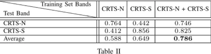
CRTS-N 0.764 0.442 0.746

CRTS-S 0.412 0.856 0.825

Average 0.588 0.649 0.786

Table II

PERFORMANCESUMMARY OF THE PROPOSED MULTI-VIEW CLASSIFICATION FRAMEWORK INCRTSLIGHT CURVE COLLECTION USING AVERAGEAUCSCORES OVER ALL CLASSES OFCRTS-NAND

CRTS-SSURVEYS.

resulting performance, in this work our primarily goal is to evaluate the framework and therefore we have used only a lower dimensional (d= 8) descriptor consisting of a small set of computationally efficient, statistical measures, to define each light curve. For example, the light curves being represented in terms of brightness variations (expressed here in the traditional inverse logarithmic scale - Mags), as a function of time (expressed here in days - MJD). While the timestamps in these raw data are different for different light curves, the proposed feature processing step is initiated by computing the difference curve of length pi

2

for each xi of length pi. For this dataset, we have xi = [xM AGi ,xM J Di ] and its corresponding difference curve is represented asdxi= [dxM AGi , dxM J Di ].

dxM J D

i is aggrregated within a binned window B =

[₁₄₅1 ,₁₄₅2 ,₁₄₅3 ,₁₄₅4 ,₂₅1,₂₅2,₂₅3,1.5,2.5,3.5,4.5,5.5,7,10,20, 30,60,90,120,240,480,720,960,2000,3000,4000,5000], which can be represented as:

dxM AG_i,j = k, s. t.dxM AG_i [k]∈Bj

(6)

dxM J D_i,j =

dxM J D_i [k], s. t.k∈dxM AG_i,j

where Bj = [B[j − 1],B[j]], a window ranged within two consecutive entries B[j −1] and B[j]. For example,

B1 = [₁₄₅1 ,₁₄₅2 ] and B7 = [₂₅3,1.5]. Then, we

com-pute fi,j = [fi,j1 , f

2 i,j, f 3 i,j, f 4 i,j, f 5 i,j, f 6 i,j, f 7 i,j,f 8 i,j] where, 8 statistical measures including mean, min, max, standard deviation, range cmulative sum, kurtosis, skew and mean absolute deviations are respectively computed for dxM J D

i,j This results in representing each xi in terms of an ordered sequence fi with T = 27 time steps. At each time step

j, we have a d = 8 dimensional response fi,j. In case of UCI Daily Sports and Activity dataset analysis, each activity is represented in terms of 60 segments spanning

over5 minutes. Therefore, in this case, the difference curve computation followed by binning formalization (as described in Equation (6)) is not required as a part of the feature processing. As such, we directly compute the statistical features describing each segment.

The stacked LSTM model representing a specific viewv∈ V, hasL= 3LSTM layers. Each of these layers is followed by an immediately following drop-out layer. The number of hidden units in each of the LSTM layers is set to be 128, while the dropout ratio for each of their corresponding dropout layers is set to be 0.2. Each FC layer of the multi-view deep classification module, is designed with 128units and defined with Rectified Linear unit (ReLU) activation. In order to reduce the risk of overfitting, each FC layer is followed by a dropout layer with its dropout ratio fixed as

κ= 0.5. Figure 1(b) illustrates the architecture of a single-view classifier. The learning of each single-view-specific stacked LSTM model occurs with80epochs and20%of the training samples are used for validation at every learning epoch. C. Results

1) Light Curve Classification: In order to handle the large variances in sample populations representing different classes, the same set of experiments is performed multiple times and the average performance details are reported in Table II and Table III. In this work, we use the Receiver Operating Characteristic (ROC) curve for evaluation. Unlike overall accuracy scores for pairwise binary classification performances reported by Mahabal et. al. [22], which is dependent on one specific cut-point, the ROC curve inves-tigates the performance of the multi-class classification task at a broader range, trying several cut-points to analyze the pattern of changes observed for False Positive Rate with varying True Positive Rate. The Area Under Curve (AUC) scores computed for these ROC curves are therefore found to be more insightful and useful as the evaluation metric.

In order to evaluate the view-invariant expressiveness capacity of the proposed framework, the performance of the proposed multi-view framework was investigated at several different experimental settings. As seen in the tables I, II, and III, single-view classifiers perform well in identifying test samples from its corresponding view, it is not equiv-alently robust in classifying samples across views. How-ever, the propose multi-view classifer proves to be equally competitive in categorizing samples across different surveys (views).

CRTS/PTF Collections: Two different 2-view settings are investigated in this part of experiments: (1) CRTS-N, PTF and (2) CRTS-N, CRTS-S. While there may be an overlap in the objects present in any of the training collection of CRTS-N, CRTS-S or PTF, information on a query object is always available from a single view-perspective. The same set of experiments is repeated10times and Table I describes the average performance of the proposed framework in

hhh_hhh

hhh_hhh

Test Band

Training Set Bands

‘G’ ‘BP’ ‘RP’ ‘G’+’BP’ ‘G’+’RP’ ‘BP’+’RP’ ‘G’+’BP’+’RP’ ‘G’ 0.91 0.87 0.86 0.92 0.92 0.88 0.93 ‘BP’ 0.81 0.89 0.84 0.84 0.82 0.89 0.87 ‘RP’ 0.81 0.83 0.88 0.83 0..87 0.88 0.88 Average 0.84 0.86 0.86 0.86 0.87 0.88 0.89 Table III

PERFORMANCESUMMARY OF THE PROPOSED MULTI-VIEW FRAMEWORK INGAIADR2LIGHT CURVE COLLECTION USING AVERAGEAUCSCORES OVER ALL CLASSES.

Method CCA MvDA MDBP Proposed Method Accuracy 0.601 0.859 0.913 0.949

Table IV

COMPARATIVESTUDY ONUCI DAILYSPORTS ANDACTIVITY DATASET,WHERE THE PROPOSED METHOD IS COMPARED AGAINST

CCA [27] MVDA [17],ANDMDBP [28].

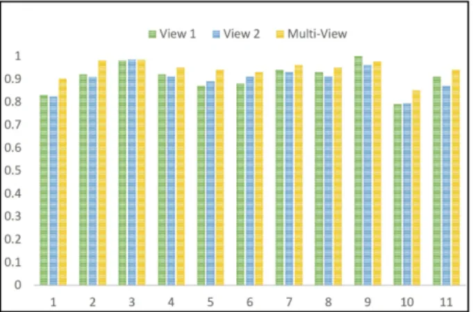
Figure 3. Summarized Performance study of the proposed multi-view learning framework in UCI Daily and Sports Activity Dataset. The activities indexed along x-axis are as follows: 1.Sitting(A1), 2.Standing(A2, A7), 3. Lying(A3, A4), 4.Going up and down the staircase(A5, A6), 5.Walking (A8, A9), 6. Walking on a treadmill(A10, A11), 7. Running(A12), 8. Exercising(A13, A14), 9.Cycling(A15, A16), 10.Rowing(A17) and 11. Jumping(A18, A19)

a 2-view setting, where samples from CRTS-N and PTF form two independent views. The performance details by considering CRTS-N and CRTS-S as two independent views are reported in Table II. As observed, while single view classifiers learned only on the CRTS-N or CRTS-S training set deteriorate drastically when classifying the samples from another view (i.e. CRTS-S or CRTS-N), the multi-view model is found to be very stable and reports an equivalent performance on test samples from both independent views. Gaia DR2 Collection:In order to check the performance of the proposed multi-view approach, we adopt multiple 2/3-view settings in our experiments, where ’G’, Gaia-’BP’, and Gaia-’RP’ constitute three independent views of the system. Table III uses mean AUC scores (computed over all classes available in the test collection) to summarize the

average performance in several multi-view settings. In order to minimize the effect of any bias due to a specific choice of training/test collection, the same set of experiments is performed 10 times and the average scores are reported in the table. As reported in the table, multi-view classi-fiers show more stable performance by reporting improved average AUC scores (e.g., 0.89 AUC achieved in the 3-view setting) over all the test samples across all the bands, compared to an average AUC score of 0.84, 0,86 and 0.86 achieved by the single view classifiers representing the bands ‘G’, ‘BP’, and ‘RP’, respectively. For example, the two-view classifier ‘G’+’RP’ reports an average of 2% improvement over the average AUC scores compared to its single-view counterparts ‘G’ and ‘RP’ and the three-view classifier shows around3%improvement over all three single view classifiers available in this experimental setting. It is important to note that, once again, the performance of single-view classifiers (specifically the classifier learned for band ‘G’) deteriorates in identifying the signals generated from other bands, while the multi-view classifier, which enables phased learning in a distributed environment, shows an impressive generalization ability and proves to be more efficient and stable in identifying samples across multiple bands without requiring its specific band information for classification.

2) Daily Activity and Sports Recognition: In order to investigate the performance of the proposed deep multi-view framework, we follow [28] to design a two-multi-view experimental setting on the UCI Daily and Sports Activity dataset. Specifically the first 27 sensors on torso, right arm and left arm are treated as View-1, while the remaining 18 sensors on right leg and left leg as View-2. In this application setting, the activities are observed from two distinct views (i.e., two groups of sensors) simultaneously. The training set consists of 400 samples representing each activity type from4subjects and a test collection is built using the activity samples collected similarly from the other 4 subjects. The AUC scores summarized in the bar graph shown in Figure 3, prove the effectiveness of the proposed multi-view approach over the single-view classifiers by displaying an effective classification performance across all the classes. The same experiment is repeated10times by selecting a different set of 4subjects in the training set that consists of a different set of

random50samples per segment and subject for each activity. Table IV reports the average accuracy scores for comparing the performance of the proposed approach in the UCI Daily Sports and Activity dataset, against several state-of-the art results reported by Li et al. [28]. Accuracy is an evaluation metric that computes the ratio of the correct predictions over all the predictions made by a classifier. By demostrating an improvement of around4% in the average accuracy, the proposed method shows significant promise compared to the state-of-the-art performance in classifying the activity patterns in this dataset. Also it is important to note that, in contrast to [28], where the authors learn the optimized latent subspace for designing a discriminative representative by utilizing the entire multi-view data repositories, the proposed method enables learning within a more distributed learning framework, which makes it more easily adaptable for several practical application settings.

V. CONCLUSION

In this paper, we present an effective, view, multi-variate deep classification model for time-series data. The proposed model derives a bilinear factor pooling scheme to effectively fuse view-specific context-aware signal rep-resentatives that weigh the most relevant feature dimensions while eliminating noise for an improved classification per-formance. Compared to many existing methods designed for multivariate time series data, the proposed method shows considerable performance improvement by efficiently mod-eling the multi-view interactions within a compact descrip-tor, which enables the system achieve a new state-of-the-art performance on the real-world datasets. The proposed model also demonstrates a more generalized expressive capacity, and therefore, is applicabile to a wide range of application scenarios and data.

ACKNOWLEDGMENT

Funding for this research was provided by the National Science Foundations (NSF) Data Infrastructure Building Blocks (DIBBs) Progam under award#1640818.

REFERENCES

[1] J. Lu, J. Yang, D. Batra, and D. Parikh, “Hierarchical question-image co-attention for visual question answering,” inAdvances in Neural Information Processing Systems 29, D. D. Lee, M. Sugiyama, U. V. Luxburg, I. Guyon, and R. Garnett, Eds. Curran Associates, Inc., 2016, pp. 289– 297. [Online]. Available: http://papers.nips.cc/paper/6202-hierarchical-question-image-co-attention-for-visual-question-answering.pdf

[2] L. Piras and G. Giacinto, “Information fusion in content based image retrieval: A comprehensive overview,”Information Fusion, vol. 37, pp. 50– 60, 09/2017 2017.

[3] S. Seto, W. Zhang, and Y. Zhou, “Multivariate time series classification using dynamic time warping template selection for human activity recog-nition,”2015 IEEE Symposium Series on Computational Intelligence, pp. 1399–1406, 2015.

[4] P.-F. Marteau and S. Gibet, “On recursive edit distance kernels with appli-cation to time series classifiappli-cation,”IEEE transactions on neural networks and learning systems, vol. 26, no. 6, June 2015.

[5] J. Lines and A. Bagnall, “Time series classification with ensembles of elastic distance measures,”Data Min. Knowl. Discov., vol. 29, no. 3, pp. 565–592, May 2015.

[6] J. Paparrizos and L. Gravano, “k-shape: Efficient and accurate clustering of time series,”SIGMOD Rec., vol. 45, no. 1, pp. 69–76, Jun. 2016. [7] Z. Fang and Z. Zhang, “Simultaneously combining view

multi-label learning with maximum margin classification,” in2012 IEEE 12th International Conference on Data Mining, 2012, pp. 864–869.

[8] S. Sun, “A survey of multi-view machine learning,”Neural Computing and Applications, vol. 23, no. 7, pp. 2031–2038, Dec 2013.

[9] J. B. Tenenbaum and W. T. Freeman, “Separating style and content,” in Advances in Neural Information Processing Systems 9, M. C. Mozer, M. I. Jordan, and T. Petsche, Eds., 1997, pp. 662–668. [Online]. Available: http://papers.nips.cc/paper/1290-separating-style-and-content.pdf [10] T. Y. Lin, A. RoyChowdhury, and S. Maji, “Bilinear cnn models for

fine-grained visual recognition,” in2015 IEEE International Conference on Computer Vision (ICCV), 2015, pp. 1449–1457.

[11] C. Orsenigo and C. Vercellis, “Combining discrete svm and fixed cardi-nality warping distances for multivariate time series classification,”Pattern Recogn., vol. 43, no. 11, pp. 3787–3794, 2010.

[12] X. Weng and J. Shen, “Classification of multivariate time series using two-dimensional singular value decomposition,” Knowledge-Based Systems, vol. 21, no. 7, pp. 535 – 539, 2008.

[13] O. Maimon and L. Rokach,Data Mining and Knowledge Discovery Hand-book. Berlin, Heidelberg: Springer-Verlag, 2005.

[14] Y. Zheng, Q. Liu, E. Chen, Y. Ge, and J. L. Zhao, “Time series classification using multi-channels deep convolutional neural networks,” in Web-Age Information Management, F. Li, G. Li, S.-w. Hwang, B. Yao, and Z. Zhang, Eds. Springer International Publishing, 2014, pp. 298–310.

[15] F. Karim, S. Majumdar, H. Darabi, and S. Harford, “Multivariate lstm-fcns for time series classification,”CoRR, vol. abs/1801.04503, 2018. [16] M. L¨angkvist, L. Karlsson, and A. Loutfi, “A review of unsupervised

feature learning and deep learning for time-series modeling,” Pattern Recognition Letters, pp. 11–24, 2014.

[17] M. Kan, S. Shan, H. Zhang, S. Lao, and X. Chen, “Multi-view discriminant analysis,”IEEE Trans. Pattern Anal. Mach. Intell., vol. 38, no. 1, pp. 188– 194, Jan. 2016.

[18] S. Li, M. Shao, and Y. Fu, “Multi-view low-rank analysis with applications to outlier detection,”ACM Trans. Knowl. Discov. Data, vol. 20, no. 3, pp. 32:1–32:22, 2018.

[19] R. Pascanu, C¸ . G¨ulc¸ehre, K. Cho, and Y. Bengio, “How to construct deep recurrent neural networks,”CoRR, vol. abs/1312.6026, 2013.

[20] S. Hochreiter and J. Schmidhuber, “Long short-term memory,”Neural Comput., vol. 9, no. 8, pp. 1735–1780, Nov. 1997.

[21] Y. Li, N. Wang, J. Liu, and X. Hou, “Factorized bilinear models for image recognition,”CoRR, vol. abs/1611.05709, 2016.

[22] A. Mahabal, K. Sheth, F. Gieseke, A. Pai, S. G. Djorgovski, A. Drake, M. Graham, and the CSS/CRTS/PTF Collaboration, “Deep-learnt clas-sification of light curves,” IEEE Symposium Series on Computational Intelligence (SSCI), vol. arXiv:1709.06257, 2017.

[23] A. J. Drake, S. G. Djorgovski, M. Catelan, M. J. Graham, A. A. Mahabal, S. Larson, E. Christensen, G. Torrealba, E. Beshore, R. H. McNaught, G. Garradd, V. Belokurov, and S. E. Koposov, “The catalina surveys southern periodic variable star catalogue,”Monthly Notices of the Royal Astronomical Society, vol. 469, no. 3, pp. 3688–3712, 2017.

[24] N. Law, S. Kulkarni, R. Dekany, and E. e. Ofek, “The palomar transient factory: System overview, performance, and first results,”PUBLICATIONS OF THE ASTRONOMICAL SOCIETY OF THE PACIFIC, vol. 121, no. 886, pp. 1395–1408, 2009.

[25] A. Brown, A. Vallenari, T. Prusti, J. de Bruijne, C. Babusiaux, and C. Bailer-Jones, “Gaia data release 2. summary of the contents and survey properties,”AA Special Issue on Gaia DR2.

[26] B. Barshan and M. C. Y ˜Aksek, “Recognizing daily and sports activities in two open source machine learning environments using body-worn sensor units,”The Computer Journal, vol. 57, no. 11, pp. 1649–1667, 2014. [27] H. Hotelling,Relations Between Two Sets of Variates. New York, NY:

Springer New York, 1992, pp. 162–190.

[28] S. Li, Y. Li, and Y. Fu, “Multi-view time series classification: A discrim-inative bilinear projection approach,” in Proceedings of the 25th ACM International on Conference on Information and Knowledge Management, ser. CIKM ’16, 2016, pp. 989–998.