HAL Id: hal-01842514
https://hal.archives-ouvertes.fr/hal-01842514v2
Submitted on 3 Sep 2019
HAL
is a multi-disciplinary open access
archive for the deposit and dissemination of
sci-entific research documents, whether they are
pub-lished or not. The documents may come from
teaching and research institutions in France or
abroad, or from public or private research centers.
L’archive ouverte pluridisciplinaire
HAL, est
destinée au dépôt et à la diffusion de documents
scientifiques de niveau recherche, publiés ou non,
émanant des établissements d’enseignement et de
recherche français ou étrangers, des laboratoires
publics ou privés.
Contrast function estimation for the drift parameter of
ergodic jump diffusion process
Chiara Amorino, Arnaud Gloter
To cite this version:
Chiara Amorino, Arnaud Gloter. Contrast function estimation for the drift parameter of ergodic jump
diffusion process. 2019. �hal-01842514v2�
Contrast function estimation for the drift parameter of ergodic
jump diffusion process.
Chiara Amorino
1and Arnaud Gloter
11
Laboratoire de Mathématiques et Modélisation d’Evry, Université Paris-Saclay
September 3, 2019
Abstract
In this paper we consider an ergodic diffusion process with jumps whose drift coefficient depends on an unknown parameter. We suppose that the process is discretely observed. We introduce an estimator based on a contrast function, which is efficient without requiring any conditions on the rate at which the step discretization goes to zero, and where we allow the observed process to have non summable jumps. This extends earlier results where the condition on the step discretization was needed and where the process was supposed to have summable jumps. In general situations, our contrast function is not explicit and one has to resort to some approximation. In the case of a finite jump activity, we propose explicit approximations of the contrast function, such that the efficient estimation of the drift parameter is feasible. This extends the results obtained by Kessler in the case of continuous processes.
Efficient drift estimation, ergodic properties, high frequency data, Lévy-driven SDE, thresholding methods.
1
Introduction
Diffusion processes with jumps have been widely used to describe the evolution of phenomenon arising in various fields. In finance, jump-processes were introduced to model the dynamic of asset prices(Merton, 1976),(Kou,2002), exchange rates (Bates, 1996), or volatility processes (Barndorff-Nielsen & Shephard, 2001),(Eraker, Johannes, & N, 2003). Utilization of jump-processes in neuroscience can be found for instance in(Ditlevsen & Greenwood, 2013).
Practical applications of these models has lead to the recent development of many statistical methods. In this work, our aim is to estimate the drift parameter θ from a discrete sampling of the processXθ
solution to Xtθ=X0θ+ Z t 0 b(θ, Xsθ)ds+ Z t 0 σ(Xsθ)dWs+ Z t 0 Z R\{0} γ(Xsθ−)zµ˜(ds, dz),
where W is a one dimensional Brownian motion andµ˜ a compensated Poisson random measure, with a possible infinite jump activity. We assume that the process is sampled at the times(tn
i)i=0,...,nwhere the
sampling step∆n:= supi=0,...,n−1t n i+1−t
n
i goes to zero. Due to the presence of a Gaussian component,
we know that it is impossible to estimate the drift parameter on a finite horizon of time. Thus, we assume that tn→ ∞and the ergodicity of the processXθ.
Generally, the main difficulty while considering statistical inference of discretely observed stochastic pro-cesses comes from the lack of explicit expression for the likelihood. Indeed, the transition density of a jump-diffusion process is usually unknown explicitly. Several methods have been developed to circumvent this difficulty. For instance, closed form expansions of the transition density of jump-diffusions is studied in(Aït-Sahalia & Yu, 2006),(Li & Chen, 2016). In the context of high frequency observation, the asymp-totic behaviour of estimating functions are studied in(Jakobsen & Sørensen, 2017), and conditions are given to ensure rate optimality and efficiency. Another approach, fruitful in the case of high frequency observation, is to consider pseudo-likelihood method, for instance based on the high frequency approx-imation of the dynamic of the process by the one of the Euler scheme. This leads to explicit contrast functions with Gaussian structures (see e.g. (Shimizu & Yoshida, 2006),(Shimizu, 2006),(Masuda, 2013)). The validity of the approximation by the Euler pseudo-likelihood is justified by the high frequency assumption of the observations, and actually proving that the estimators are asymptotic normal usually necessitates some conditions on the rate at which∆nshould tend to zero. For applications, it is important
In the case of continuous processes, Florens-Zmirou (Florens-Zmirou, 1989)proposes estimation of drift and diffusion parameters under the fast sampling assumptionn∆2n→0. Yoshida(Yoshida, 1992)suggests a correction of the contrast function that yields to the condition n∆3n →0. In Kessler(Kessler, 1997), the author introduces an explicit modification of the Euler scheme contrast such that the associated estimators are asymptotically normal, under the condition n∆kn → 0 where k ≥ 2 is arbitrarily large.
Hence, the result by Kessler allows for any arbitrarily slow polynomial decay to zero of the sampling step. In the case of jump-diffusions, Shimizu(Shimizu, 2006)proposes parametric estimation of drift, diffusion and jump coefficients. The asymptotic normality of the estimators are obtained under some explicit conditions relating the sampling step and jump intensity of the process. These conditions on ∆n are
more restrictive as the intensity of jumps near zero is high. In the situation where this jump intensity is finite, the conditions of(Shimizu,2006)reduces ton∆2
n→0. In(Gloter, Loukianova, & Mai, 2018), the
condition on the sampling step is relaxed ton∆3
n→0, when one estimates the drift parameter only.
In this paper, we focus on the estimation of the drift parameter, and our aim is to weaken the conditions on the decay of the sampling step in way comparable to Kessler’s work(Kessler, 1997), but in the framework of jump-diffusion processes.
One of the idea in Kessler’s paper is to replace, in the Euler scheme contrast function, the contribution of the drift by the exact value of the first conditional momentm(1)θ,t
i,ti+1(x) =E[X
θ ti+1 |X
θ
ti =x]or some
explicit approximation with arbitrarily high order when ∆n → 0. In presence of jumps, the contrasts
functions in (Shimizu & Yoshida, 2006)(see also (Shimizu, 2006), (Gloter, Loukianova, & Mai, 2018)) resort to a filtering procedure in order to suppress the contribution of jumps and recover the continuous part of the process. Based on those ideas, we introduce a contrast function (see Definition 1), whose expression relies on the quantity mθ,ti,ti+1(x) =
E[Xθti +1ϕ((X θ ti+1−X θ ti)/(ti+1−ti)β)|Xtiθ=x] E[ϕ((Xθ ti+1−X θ
ti)/(ti+1−ti)β)|Xtiθ=x] , where ϕis some
compactly supported function and β <1/2. The functionϕ is such thatϕ((Xtθi+1−X
θ
ti)/(ti+1−ti) β)
vanishes when the increments of the data are too large compared to the typical increments of a continuous diffusion process, and thus can be used to filter the contribution of the jumps.
The main result of our paper is that the associated estimator converges at rate √tn, with some explicit
asymptotic variance and is efficient. Comparing to earlier results ((Shimizu & Yoshida, 2006),(Shimizu, 2006),(Gloter, Loukianova, & Mai, 2018)), the sampling step(tn
i)i=0,...,n can be irregular, no condition
is needed on the rate at which ∆n → 0 and we have suppressed the assumption that the jumps of the
process are summable. Let us stress that when the jumps activity is so high that the jumps are not summable, we have to chooseβ <1/3 (see AssumptionAβ).
Moreover, in the case where the intensity is finite and with the specific choice of ϕbeing an oscillating function, we prove that we can approximate our contrast function by a completely explicit one, exactly as in the paper by Kessler(Kessler, 1997). This yields to an efficient estimator under the conditionn∆kn→0,
wherekis related to the oscillating properties of the functionϕ. Askcan be chosen arbitrarily high, up to a proper choice ofϕ, our method allows to estimate efficiently the drift parameter, under the assumption that the sampling step tends to zero at some polynomial rate.
We also show numerically that, when the jump activity is finite, the estimator we deduce from the explicit approximation of the contrast function performs well, making the bias visibly reduced.
On the other side, considering the case of infinite jumps activity (taking in particular a temperedα-stable jump process withα <1), we implement our main results building an approximation ofm(see Theorem
2 below) from which we deduce an approximation of the contrast that we minimize in order to get the estimator of the drift coefficient. The estimator we found is a corrected version of the estimator that would result from the choice of an Euler scheme approximation. We see numerically that our estimator is well-performed and that the correction term we give drastically reduces the bias, especially as αgets bigger.
The outline of the paper is the following. In Section 2 we present the assumptions on the process X. The Section3contains the main results of the paper: in Section3.1we define the contrast function while the consistency and asymptotic normality of the estimator are stated in Section 3.2. In Section 4 we explain how to use in practice the contrast function and so we deal with its approximations in Section
4.1 while its explicit modification is presented in the case of finite jump activity in Section 4.2. The Section5is devoted to numerical results and perspectives for practical applications. In Section6we state limit theorems useful to study the asymptotic behavior of the contrast function. The proofs of the main statistical results are given in Section7, while the proofs of the limit theorems and some technical results are presented in the Appendix.
2
Model, assumptions
LetΘbe a compact subset ofRandXθ a solution to
Xtθ=X0θ+ Z t 0 b(θ, Xsθ)ds+ Z t 0 a(Xsθ)dWs+ Z t 0 Z R\{0} γ(Xsθ−)zµ˜(ds, dz), t∈R+, (1)
where W = (Wt)t≥0 is a one dimensional Brownian motion, µ is a Poisson random measure associated
to the Lévy process L= (Lt)t≥0, with Lt:= Rt
0 R
Rzµ˜(ds, dz)andµ˜ =µ−µ¯ is the compensated one, on
[0,∞)×R. We denote(Ω,F,P)the probability space on whichW andµare defined.
We suppose that the compensator has the following form: µ¯(dt, dz) :=F(dz)dt, where conditions on the Levy measureF will be given later.
The initial condition Xθ
0,W andL are independent.
2.1
Assumptions
We suppose that the functionsb: Θ×R→R,a:R→Randγ:R→Rsatisfy the following assumptions:
ASSUMPTION 1: The functions a(x), γ(x) and, for all θ ∈ Θ, b(x, θ) are globally Lipschitz. More-over, the Lipschitz constant of b is uniformly bounded onΘ.
Under Assumption 1 the equation (1) admits a unique non-explosive càdlàg adapted solution possessing the strong Markov property, cf(Applebaum, 2009)(Theorems 6.2.9. and 6.4.6.).
ASSUMPTION 2: For all θ ∈ Θ there exists a constant t > 0 such that Xθ
t admits a density pθt(x, y)
with respect to the Lebesgue measure on R; bounded in y ∈R and in x∈K for every compact K ⊂R. Moreover, for every x∈Rand every open ball U ∈R, there exists a point z =z(x, U)∈supp(F) such that γ(x)z∈U.
The last assumption was used in (Masuda, 2007) to prove the irreducibility of the process Xθ. Other
sets of conditions, sufficient for irreducibility, are in(Masuda, 2007). ASSUMPTION 3 (Ergodicity):
1. For allq >0,R|z|>1|z|qF(z)dz <∞.
2. For allθ∈Θthere existsC >0 such that xb(x, θ)≤ −C|x|2, if|x| → ∞.
3. |γ(x)|/|x| →0 as|x| → ∞. 4. |a(x)|/|x| →0as|x| → ∞.
5. ∀θ∈Θ,∀q >0we have E|X0θ|q<∞.
Assumption 2 ensures, together with the Assumption 3, the existence of unique invariant distributionπθ, as well as the ergodicity of the processXθ, as stated in the Lemma2 below.
ASSUMPTION 4 (Jumps):
1. The jump coefficientγ is bounded from below, that isinfx∈R|γ(x)|:=γmin>0.
2. The Lévy measure F is absolutely continuous with respect to the Lebesgue measure and we denote
F(z) =F(dz)dz .
3. We suppose that ∃c >0 s.t., for allz∈R,F(z)≤|z|1+c α, withα∈(0,2).
Assumptions 4.1 is useful to compare size of jumps of X andL.
ASSUMPTION 5 (Non-degeneracy): There exists someα >0, such thata2(x)≥αfor allx∈
R
The Assumption 5ensures the existence of the contrast function defined in Section3.1. ASSUMPTION 6 (Identifiability): For allθ6=θ0,(θ, θ0)∈Θ2,
Z
R
(b(θ, x)−b(θ0, x))2 a2(x) dπ
We can see that this last assumption is equivalent to
∀θ6=θ0, (θ, θ0)∈Θ2, b(θ, .)6=b(θ0, .). (2) We also need the following technical assumption:
ASSUMPTION 7:
1. The derivatives ∂x∂kk1 +1∂θk2kb2, with k1+k2 ≤4 andk2 ≤3, exist and they are bounded ifk1 ≥1. If k1= 0, for eachk2≤3they have polynomial growth.
2. The derivativesa(k)(x)exist and they are bounded for each1≤k≤4. 3. The derivativesγ(k)(x)exist and they are bounded for each 1≤k≤4.
Define the asymptotic Fisher information by
I(θ) = Z R (˙b(θ, x))2 a2(x) π θ(dx). (3)
ASSUMPTION 8: For all θ∈Θ,I(θ)>0.
Remark 1. If α < 1, using Assumption 4.3 the stochastic differential equation (1) can be rewritten as follows: Xtθ=X0θ+ Z t 0 ¯ b(θ, Xsθ)ds+ Z t 0 a(Xsθ)dWs+ Z t 0 Z R\{0} γ(Xsθ−)zµ(ds, dz), t∈R+, (4) where¯b(θ, Xθ s) =b(θ, Xsθ)− R R\{0}γ(X θ s−)zF(z)dz.
This expression implies that X follows diffusion equationXtθ=X0θ+ Rt 0¯b(θ, X θ s)ds+ Rt 0a(X θ s)dWsin the
interval in which no jump occurred.
From now on we denote the true parameter value byθ0, an interior point of the parameter spaceΘthat
we want to estimate. We shorten X forXθ0.
We will use some moment inequalities for jump diffusions, gathered in the following lemma:
Lemma 1. LetXsatisfies Assumptions 1-4. LetLt:= Rt
0 R
Rzµ˜(ds, dz)and letFs:=σ{(Wu)0<u≤s,(Lu)0<u≤s, X0}.
Then, for all t > s,
1) for all p≥2,E[|Xt−Xs|p]
1
p ≤c|t−s|1p,
2) for all p≥2,p∈N,E[|Xt−Xs|p|Fs]≤c|t−s|(1 +|Xs|p).
3) for all p≥2,p∈N,suph∈[0,1]E[|Xs+h|p|Fs]≤c(1 +|Xs|p).
The first two points follow from Theorem 66 of(Protter, 2005)and Proposition 3.1 in(Shimizu & Yoshida, 2006). The last point is a consequence of the second one: ∀h∈[0,1],
E[|Xs+h|p|Fs] =E[|Xs+h−Xs+Xs|p|Fs]≤c(E[|Xs+h−Xs|p|Fs] +E[|Xs|p|Fs]),
where cmay change value line to line. Using the second point of Lemma 1and the measurability of Xs
with respect to Fs, it is upper bounded byc|h|(1 +|Xs|p) +c|Xs|p. Therefore
sup
h∈[0,1]
E[|Xs+h|p|Fs]≤ sup h∈[0,1]
c|h|(1 +|Xs|p) +c|Xs|p≤c(1 +|Xs|p).
2.2
Ergodic properties of solutions
An important role is playing by ergodic properties of solution of equation (1)
The following Lemma states that Assumptions1−4are sufficient for the existence of an invariant measure
πθ such that an ergodic theorem holds and moments of all order exist.
Lemma 2. Under assumptions 1 to 4, for allθ∈Θ,Xθ admits a unique invariant distribution πθ and
the ergodic theorem holds:
1. For every measurable functiong:R→Rsatisfying πθ(g)<∞, we have a.s.
lim t→∞ 1 t Z t 0 g(Xsθ)ds=πθ(g).
2. For allq >0,πθ(|x|q)<∞.
3. For allq >0,supt≥0E[|Xtθ| q]<∞.
A proof is in (Gloter, Loukianova, & Mai, 2018) (Section 8 of Supplement) in the caseα ∈(0,1), the proof relies on (Masuda, 2007). In order to use it also in the caseα ≥1 we have to show that, taken
q >2 qeven andf?(x) =|x|q, f? satisfies the drift conditionAf? =A
df?+Acf? ≤ −c1f?+c2, where c1>0 andc2>0.
Using Taylor’s formula up to second order we have
|Adf?(x)| ≤c Z R Z 1 0 |z|2kγk ∞|f 00?(x+szγ(y))|F(z)dsdz= =c Z R Z 1 0 |z|2kγk ∞q(q−1)|x+szγ(y)| q−2F(z)dsdz=o(|x|q). (5)
Concerning the generator’s continuous part, we use the second point of Assumption 3 to get
Acf?(x) =
1 2σ
2(x)q(q−1)xq−2+b(θ, x)q x xq−2≤o(|x|q)−cq|x|2xq−2≤o(|x|q)−cf?(x). (6)
By (5) and (6), the drift condition holds.
3
Construction of the estimator and main results
We exhibit a contrast function for the estimation of a parameter in the drift coefficient. We prove that the derived estimator is consistent and asymptotically normal.
3.1
Construction of the estimator
LetXθbe the solution to (1). Suppose that we observe a finite sample Xt0, ..., Xtn; 0 =t0≤t1≤...≤tn,
where X is the solution to (1) with θ = θ0. Every observation time point depends also on n, but to
simplify the notation we suppress this index. We will be working in a high-frequency setting, i.e.
∆n:= sup i=0,...,n−1
∆n,i−→0, n→ ∞,
with∆n,i:= (ti+1−ti).
We assume limn→∞tn =∞andn∆n=O(tn)asn→ ∞.
We introduce a jump filtered version of the gaussian quasi-likelihood. This leads to the following contrast function:
Definition 1. Forβ ∈(0,12)andk >0, we define the contrast functionUn(θ)as follows:
Un(θ) := n−1 X i=0 (Xti+1−mθ,ti,ti+1(Xti)) 2 a2(X ti)(ti+1−ti) ϕ∆β n,i (Xti+1−Xti)1{|Xti|≤∆−n,ik} (7) where mθ,ti,ti+1(x) := E[Xtiθ+1ϕ∆βn,i(X θ ti+1−X θ ti)|Xtiθ =x] E[ϕ∆βn,i(X θ ti+1−X θ ti)|X θ ti =x] (8) and ϕ∆β n,i (Xti+1−Xti) =ϕ( Xti+1−Xti ∆βn,i ),
with ϕ a smooth version of the indicator function, such that ϕ(ζ) = 0 for each ζ, with |ζ| ≥ 2 and
ϕ(ζ) = 1for each ζ, with |ζ| ≤1.
The last indicator aims to avoid the possibility that |Xti| is big. The constantkis positive and it will be
choosen later, related to the development of mθ,ti,ti+1(x)(cf. Remark2 below).
Moreover we define
mθ,h(x) :=E
[Xhθϕhβ(Xhθ−X0θ)|X0θ=x]
E[ϕhβ(Xhθ−X0θ)|X0θ=x] .
By the homogeneity of the equation we get thatmθ,ti,ti+1(x)depends only on the differenceti+1−ti and so mθ,ti,ti+1(x) =mθ,ti+1−ti(x)that we may denote simply asmθ(x), in order to make the notation easier.
We define an estimatorθˆn ofθ0as
ˆ
θn∈argmin
θ∈ΘUn(θ). (9)
The idea, with a finite intensity, is to use the size ofXti+1−Xtiin order to judge the existence of a jump
in an interval[ti, ti+1). The increment ofX with continuous transition could hardly exceed the threshold
∆βn,i withβ∈(0,1
2). Therefore we can judge a jump occurred if|Xti+1−Xti|>∆
β
n,i. We keep the idea
even when the intensity is no longer finite.
With a such defined mθ(Xti), using the true parameter valueθ0, we have that
E[(Xti+1−mθ0,ti,ti+1(Xti))ϕ∆βn,i(Xti+1−Xti)|Xti =x] =E[Xti+1ϕ∆n,iβ (Xti+1−x)|Xti =x]+
−E
[Xti+1ϕ∆βn,i(Xti+1−Xti)|Xti =x]
E[ϕ∆βn,i(Xti+1−Xti)|Xti =x]
E[ϕ∆βn,i(Xti+1−Xti)|Xti=x] = 0,
where we have just used the definition and the measurability of mθ0,ti,ti+1(Xti).
But, as the transition density is unknown, in general there is no closed expression formθ,h(x), hence the
contrast is not explicit. However, in the proof of our results we will need an explicit development of (7). In the sequel, for δ ≥0, we will denote R(θ,∆δ
n,i, x) for any function R(θ,∆n,iδ , x) = Ri,n(θ, x), where Ri,n: Θ×R−→R,(θ, x)7→Ri,n(θ, x)is such that
∃c >0 |Ri,n(θ, x)| ≤c(1 +|x|c)∆δn,i (10)
uniformly inθand withc independent ofi, n.
The functions R represent the term of rest and have the following useful property, consequence of the just given definition:
R(θ,∆δn,i, x) = ∆δn,iR(θ,∆0n,i, x). (11)
We point out that it does not involve the linearity ofR, since the functionsRon the left and on the right side are not necessarily the same but only two functions on which the control (10) holds with∆δn,i and
∆0
n,i, respectively.
We state asymptotic expansions for mθ,∆n,i. The cases α < 1 and α ≥ 1 yield to different
magni-tude for the rest term.
Case α∈(0,1):
Theorem 1. Suppose that Assumptions 1 to 4 hold and that β ∈ (0,12) and α ∈ (0,1) are given in definition 1 and the third point of Assumption4, respectively. Then
E[ϕ∆βn,i(X θ ti+1−X θ ti)|X θ ti=x] = 1 +R(θ,∆ (1−α β)∧(2−3β) n,i , x). (12)
Theorem 2. Suppose that Assumptions 1 to 4 hold and that β ∈ (0,1
2) and α ∈ (0,1) are given in
definition 1 and the third point of Assumption4, respectively. Then
E[(Xtiθ+1−x)ϕ∆βn,i(X θ ti+1−X θ ti)|X θ ti =x] = ∆n,ib(x, θ)+ (13) −∆n,i Z R\{0} z γ(x) [1−ϕ∆β n,i (γ(x)z)]F(z)dz + R(θ,∆2n,i−2β, x).
There existsk0>0such that, for|x| ≤∆−n,ik0,
mθ,∆n,i(x) =x+ ∆n,ib(x, θ)+ (14) −∆n,i Z R\{0} z γ(x) [1−ϕ∆β n,i(γ(x)z)]F(z)dz + R(θ,∆ 2−2β n,i , x). . Case α∈[1,2):
Theorem 3. Suppose that Assumptions 1 to 4 hold and that β ∈ (0,1
2) and α ∈ [1,2) are given in
definition 1 and the third point of Assumption4, respectively. Then
E[ϕ∆βn,i(X θ ti+1−X θ ti)|X θ ti=x] = 1 +R(θ,∆ (1−αβ)∧(2−4β) n,i , x). (15)
Theorem 4. Suppose that Assumptions 1 to 4 hold and that β ∈ (0,13) and α ∈ [1,2) are given in definition 1 and the third point of Assumption4, respectively. Then
E[(Xtθi+1−x)ϕ∆βn,i(X θ ti+1−X θ ti)|X θ ti =x] = ∆n,ib(x, θ)+ (16) −∆n,i Z R\{0} z γ(x) [1−ϕ∆β n,i (γ(x)z)]F(z)dz + R(θ,∆2n,i−3β, x).
There existsk0>0such that, for|x| ≤∆−n,ik0,
mθ,∆n,i(x) =x+ ∆n,ib(x, θ)+ (17) −∆n,i Z R\{0} z γ(x) [1−ϕ∆β n,i (γ(x)z)]F(z)dz + R(θ,∆2n,i−3β, x).
Remark 2. The constantk in the definition (7)of contrast function can be taken in the interval(0, k0].
In this way ∆−n,ik ≤∆−k0
n,i and so (14)or (17)holds for |x|=|Xti|smaller than∆−n,ik.
If it is not the case the contribution of the observation Xti in the contrast function is just 0. However
we will see that suppressing the contribution of too big|Xti|does not effect the efficiency property of our
estimator.
Remark 3. In the development (13) or (16) the term ∆n,i RR\{0}z γ(x) [1−ϕ∆β n,i
(γ(x)z)]F(z)dz is independent ofθ, hence it will disappear in the differencemθ(x)−mθ0(x), but it is not negligible compared
to∆n,ib(x, θ)since its order is∆n,i ifα∈(0,1)and at most∆
1 2
n,i ifα∈[1,2). Indeed, by the definition
of the function ϕ, we know that we can consider as support of ϕ∆β n,i (0)−ϕ∆β n,i (γ(x)z) the interval c×[−∆ β n,i kγk∞, ∆βn,i kγk∞]
c. If α < 1, using moreover the third point of Assumption 4 we get the following
estimation: |∆n,i Z R\{0} z γ(x) [1−ϕ∆β n,i (γ(x)z)]F(z)dz| ≤R(θ0,∆1n,i, Xti). (18) Otherwise, ifα≥1, we have |∆n,i Z R\{0} z γ(x) [1−ϕ∆β n,i (γ(x)z)]F(z)dz| ≤c|∆n,i| Z c×[−∆ β n,i kγk∞, ∆βn,i kγk∞]c |z|−α=R(θ,∆1+β(1−α) n,i , x),
with β∈(0,12)andα∈[1,2), hence the exponent on ∆n,i is always more than 12.
We can therefore write in the first case
mθ,∆n,i(x) =x+R(θ,∆n,i, x) =R(θ,∆0n,i, x) (19)
and in the second
mθ,∆n,i(x) =x+R(θ,∆
1+β(1−α)
n,i , x) =R(θ,∆ 0
n,i, x). (20) Remark 4. In Theorems1- 3we do not need conditions on β because, for eachβ∈(0,1
2)and for each α∈(0,2) the exponent on ∆n,i is positive and therefore the last term of (15) is negligible compared to
1. In Theorem 4, instead, R is a negligible function if and only if 2−3β ≥1, it means that it must be
β ≤1
3. We have takenβ∈(0, 1
3)and so such a condition is always respected.
3.2
Main results
Let us introduce the AssumptionAβ that turns out starting from Theorems 1,2,3and4:
ASSUMPTION Aβ: We choose β ∈ (0,12) if α ∈ (0,1). If on the contrary α ∈ [1,2), then we take β in(0,13).
The following theorems give a general consistency result and the asymptotic normality of the estimator
ˆ
θn, that hold without further assumptions on nand∆n. Theorem 5. (Consistency)
Suppose that Assumptions 1 to 7 and Aβ hold and let k of the definition of the contrast function (7) be
in (0, k0). Then the estimator θˆn is consistent in probability:
ˆ
θn−→P θ0, n→ ∞.
Theorem 6. (Asymptotic normality)
Suppose that Assumptions 1 to 8 and Aβ hold, and0< k < k0.
Then the estimator θˆn is asymptotically normal:
√
tn(ˆθn−θ0)
L
−→N(0, I−1(θ0)), n→ ∞.
Remark 5. Furthermore, the estimatorθˆn is asymptotically efficient in the sense of the Hájek-Le Cam
convolution theorem.
The Hájek−LeCam convolution theorem states that any regular estimator in a parametric model which satisfies LAN property is asymptotically equivalent to a sum of two independent random variables, one of which is normal with asymptotic variance equal to the inverse of Fisher information, and the other having arbitrary distribution. The efficient estimators are those with the second component identically equal to zero.
The model (1) is LAN with Fisher information I(θ) = R
R
( ˙b(θ,x))2
a2(x) πθ(dx) (see (Gloter, Loukianova, &
Mai, 2018)) and thusθˆn is efficient.
Remark 6. We point out that, contrary to the papers (Gloter, Loukianova, & Mai, 2018)and(Shimizu & Yoshida, 2006), in this case there is not any condition on the sampling, that can be irregular and with
∆n that goes slowly to zero. On the other hand, our contrast function relies on the quantity mθ,h(x)
which is not explicit in general.
4
Practical implementation of the contrast method
In order to use in practice the contrast function (7), one need to know the values of the quantities
mθ,ti,ti+1(Xti). In most cases, it seems impossible to find an explicit expression for the functionmθ,h
appearing in Definition1. However, explicit or numerical approximations of this function seem available in many situations.
4.1
Approximate contrast function
Let us assume that one has at disposal an approximation of the function mθ,h(x), denoted by meθ,h(x)
which satisfies, for|x| ≤h−k0,
|meθ,h(x)−mθ,h(x)| ≤R(θ, hρ, x)
where the constant ρ > 1 assesses the quality of the approximation. We assume that the first three derivatives of m˜h,θ with respect to the parameter provide approximation of the derivatives ofmh,θ, in
the following way
|∂ i e mθ,h(x) ∂θi − ∂imθ,h(x) ∂θi | ≤R(θ, h 1+, x), fori= 1,2, (21) |∂ 3 e mθ,h(x) ∂θ3 − ∂3m θ,h(x) ∂θ3 | ≤R(θ, h, x), (22)
for all |x| ≤h−k0 and where >0. Let us stress that from Proposition8 below, we know the derivatives
with respect to θof the quantitymh,θ.
Now, we consider eθn the estimator obtained from minimization of the contrast function (7) where one
has replaced mθ,ti,ti+1(Xti)by its approximation meθ,∆n,i(Xti). Then, the result of Theorem 6 can be
extended as follows.
Proposition 1. Suppose that Assumptions 1 to 8 andAβhold, with0< k < k0, and that
√
n∆ρn−1/2→0
asn→ ∞.
Then, the estimatorθen is asymptotically normal:
√
tn(θen−θ0)
L
−→N(0, I−1(θ0)), n→ ∞.
We give below several examples of approximations of mθ,h. Let us stress that, in general, Theorem 2
(resp. Theorem4) provides an explicit approximation ofmθ,∆n,i(x)with an error of order∆ 2−2β n,i (resp.
of order ∆2n,i−3β). They can be used to construct an explicit contrast function. In the next section we show that when the intensity is finite, it is possible to construct an explicit approximation ofmθ,h with
4.2
Explicit contrast in the finite intensity case.
In the case with finite intensity it is possible to make the contrast explicit, using the development of
mθ,∆n,i proved in the next proposition. We need the following assumption:
ASSUMPTIONAf:
1. We haveF(z) =λF0(z), R
RF0(z)dz= 1andF is aC
∞ function.
2. We assume thatx7→a(x),x7→b(x, θ)andx7→γ(x)areC∞ functions, they have at most uniform inθ polynomial growth as well as their derivatives.
Let us define A(k)K (x) = ¯Ak
c(g)(x), with g(y) = (y−x) and A¯c(f) = ¯bf0 +12a2f00; ¯b(θ, y) = b(θ, y)− R
Rγ(y)zF(z)dzas in the Remark1.
Proposition 2. Assume that Af holds and let ϕ be a C∞ function that has compact support and such
that ϕ≡1on [−1,1]and∀k∈ {0, ..., M},R
Rx
kϕ(x)dx= 0forM ≥0. Then, for |x| ≤∆−k0
n,i with some k0>0, mθ,∆n,i(x) =x+ bβ(M+2)c X k=1 A(k)K (x)∆ k n,i k! +R(θ,∆ β(M+2) n,i , x). (23)
In order to say that (23) holds, we have to prove the existence of a function ϕwith a compact support such that ϕ≡1 on [−1,1]and, ∀k ∈ {0, ..., M}, R
Rx
kϕ(x)dx. We build it throughψ, a function with
compact support, C∞, such thatψ|
[−1,1](x) = x M
M!. We then defineϕ(x) := ∂M ∂xMψ(x).
In this way we haveϕ≡1on[−1,1],ϕisC∞, with compact support and such that for eachl∈ {0, ...M}, using the integration by parts,R
Rx
lϕ(x)dx= 0, as we wanted.
Remark 7. The development (23) is the same found in Kessler (Kessler, 1997) in the case without jumps and it is obtained by the iteration of the continuous generator A¯c. Hence, it is completely
ex-plicit. Let us stress that in Kessler (Kessler, 1997) the right hand side of (23) stands for an approx-imation of E[ ¯Xθ
∆n,i |
¯ Xθ
0 = x] where X¯θ is the continuous diffusion solution of dX¯tθ = ¯b(θ,X¯sθ)ds+ σ( ¯Xθ
s)dWs. From Proposition 2, the right hand side of (23) is also an approximation of mθ,∆n,i(x) = E[X∆θ n,iϕ∆βn,i(X θ ∆n,i−x)|X θ 0 =x] E[ϕ∆β n,i (Xθ ∆n,i−x)|X θ 0 =x]
in the case of finite activity jumps, and for a truncation kernel ϕ
satisfying ∀k ∈ {0, ..., M}, R
Rx
kϕ(x)dx = 0. We emphasize that in the expansion of m
θ,∆i,n given in
Proposition 2, the contribution of the discontinuous part of the generator disappears only thanks to the choice of an oscillating functionϕ.
Remark 8. In the definition of the contrast function (7)we can replacemθ,∆i,n(x)with the explicit
ap-proximationmekθ,∆ n,i(x) :=x+ Pk h=1 ∆hn,i h! A (h) K (x), with an errorR(θ,∆ k
n,i, x), fork≤ b2(M+1)βc. Using A(1)K (x) = ∆n,i[b(θ, x)−R
Rγ(y)zF(z)dz] and the expansions (120)–(122) we deduce that the conditions
(21)– (22)are valid. Then, by application of Proposition 1, we can see that the associated estimator is efficient under the assumption √n∆k−
1 2
n →0 forn→ ∞. As M, and thusk, can be chosen arbitrarily
large, we see that the sampling step∆n is allowed to converge to zero in a arbitrarily slow polynomial rate
as a function of n. It turns out that a slow sampling step necessitates to choose a truncation function with more vanishing moments.
5
Numerical experiments
5.1
Finite jump activity
Let us consider the model
Xt=X0+ Z t 0 (θ1Xs+θ2)ds+σWt+γ Z t 0 Z R\{0} zµ˜(ds, dz), (24)
where the compensator of the jump measure is µ(ds, dz) =λF0(z)dsdz for F0 the probability density
of the law N(µJ, σJ2) with µJ ∈ R, σJ > 0, σ > 0, θ1 < 0, θ2 ∈ R, γ ≥ 0, λ ≥ 0. Since the jump
activity is finite, we know from Section4.2that the functionm(θ1,θ2),∆n,i(x)can be approximated at any
continuous S.D.E.X¯t= ¯X0+R t
0(θ1X¯s+θ2−γλµJ)ds+σWt , which is explicit due to the linearity of
the model, we decide to directly use the expression of the conditional moment and set
e m(θ1,θ2),∆n,i(x) = (x+ θ2 θ1 −γλµJ θ1 )eθ1∆n,i+γλµJ−θ2 θ1 . (25)
Following Nikolskii (Nikolskii, 1977), we construct oscillating truncation functions in the following way. First, we chooseϕ(0) :
R→[0,1]aC∞symmetric function with support on[−2,2]such thatϕ(0)(x) = 1
for |x| ≤ 1. We let, for d >1, ϕ(1)d (x) = (dϕ(0)(x)−ϕ(0)(x/d))/(d−1), which is a function equal to 1
on [−1,1], vanishing on [−d, d]c and such that R
Rϕ
(1)
d (x)dx = 0. Forl ∈ N, l ≥ 1, and d > 1, we set ϕ(l)d (x) = c−d1Plk=1Ck
l(−1)k+1 1kϕ (1)
d (x/k), where cd = Pl
k=1Clk(−1)k+1 1k. One can check that ϕ (l) d is
compactly supported, equal to1 on[−1,1], and that for allk∈ {0, . . . , l},R
Rx
kϕ(l)
d (x)dx= 0, for l≥1.
With these notations, we estimate the parameterθ= (θ1, θ2)by minimization of the contrast function
Un(θ) = n−1 X i=0 (Xti+1−me(θ1,θ2),∆n,i(Xti)) 2ϕ(l) c∆βn,i(Xti+1−Xti), (26)
where l∈Nandc >0will be specified latter.
For numerical simulations, we choose T = 2000, n = 104, ∆
i,n = ∆n = 1/5, θ1 = −0.5, θ2 = 2 and X0=x0= 4. We estimate the bias and standard deviation of our estimators using a Monte Carlo method
based on 5000 replications. As a start, we consider a situation without jumpsλ= 0, in which we remove the truncation functionϕin the contrast, as it is useless in absence of jumps. In Table1, we compare the estimatorθen which uses the Kessler exact bias correction given by (25), with an estimator based on the
Euler scheme approximation where one uses the approximationmeEuler
(θ1,θ2),∆n,i(x) =x+∆n,i(θ1x+θ2). From
Table 1we see that the estimator θ˜Euler
n based on Euler contrast exhibits some bias which is completely
removed using Kessler’s correction. Next, we set a jump intensityλ= 0.1, with jumps size whose common law isN(0,2)and set γ= 1. We use the contrast function relying on (25). Results are given for three choices of truncation function, ϕ(0), ϕ(2)
d and ϕ (3)
d where d = 3. Plots of these functions are given in
Figure1. We chooseβ= 0.49andc= 1. As the true value of the volatility isσ= 0.3, this choice enables most of the increments without jumps of X on[ti, ti+1]to be such thatϕ
(l)
c∆βn,i(Xti+1−Xti) = 1. Let us
stress that, if σ is unknown, it is possible to estimate, even roughly, the local value of the volatility in order to choosec accordingly (see(Gloter, Loukianova, & Mai, 2018) for analogous discussion). Results in Table2 show that the estimator works well, with a reduced bias for all choices of truncation function. Especially the bias is much smaller than the one of the Euler scheme contrast in absence of jumps. It shows the benefit of using (25) in the contrast function, even if the truncation function is not oscillating as is it when we consider ϕ(0). We remark that by the choice of a symmetric truncation function one has R
Ruϕ
(0)(u)du = 0and inspecting the proof of Proposition 8 it can be seen that this conditions is
sufficient, in the expansion of mθ,∆n,i, to suppress the largest contribution of the discrete part of the
generator.
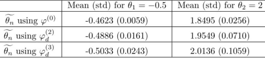
If the number of jumps is greater, e.g. for λ= 1, we see in Table 3 that using the oscillating kernels
ϕ(2)d , ϕ(3)d yields to a smaller bias than using ϕ(0), whereas it tends to increase the standard deviation
of the estimator. The estimator we get usingϕ(3)d performs well in this situation, it has a negligible bias and a standard deviation comparable to the one in the case where the process has no jump.
Mean (std) forθ1=−0.5 Mean (std) forθ2= 2
˜ θEuler
n -0.4783 (0.0213) 1.9133 (0.0856)
e
θn -0.5021 (0.0236) 2.0084 (0.0947)
Table 1: Process without jump
Mean (std) forθ1=−0.5 Mean (std) forθ2= 2 f θn usingϕ(0) -0.4967 (0.0106) 1.9869 (0.0430) f θn usingϕ (2) d -0.4990 (0.0153) 1.9959 (0.0622) f θn usingϕ (3) d -0.5006 (0.0196) 2.0023 (0.0798)
Mean (std) forθ1=−0.5 Mean (std) forθ2= 2 f θn usingϕ(0) -0.4623 (0.0059) 1.8495 (0.0256) f θn usingϕ (2) d -0.4886 (0.0161) 1.9549 (0.0710) f θn usingϕ (3) d -0.5033 (0.0243) 2.0136 (0.1059)
Table 3: Gaussian jumps withλ= 1
(a)ϕ(0) (b)ϕ(2)d withd= 3 (c)ϕ(3)d withd= 3
Figure 1: Plot of the truncation functions
5.2
Infinite jumps activity
Let us consider X solution to the stochastic differential equation (24), where the compensator of the jump measure isµ(ds, dz) =ze1+−zα1(0,∞)(z)dsdzwithα∈(0,1). This situation corresponds to the choice
of the Levy process(R0tR
R\{0}zµ˜(ds, dz))tbeing a temperedα-stable jump process. In the case of infinite
jump activity, we have no result providing approximations at any arbitrary order of mθ,∆n,i. However,
we can use Theorem 2to find some useful explicit approximation.
According to (14) and taking into account that the threshold level isc∆βn,i for somec >0, we have
mθ,∆n,i(x) =x+ ∆n,i(θ1x+θ2)−∆n,iγ Z ∞ 0 e−z zα dz+ ∆n,iγ Z ∞ 0 ϕc∆β n,i(γz) e−z zαdz+R(θ,∆ 2−2β n,i , x) =x+ ∆n,ib(x, θ1, θ2) + ∆ 1+β(1−α) n,i c 1−αγα Z ∞ 0 ϕ(v)e −cv∆ β n,i γ vα dv+R(θ,∆ 2−2β n,i , x),
where in the last line, following the notation of Remark1, we have setb(x, θ1, θ2) = (θ1x+θ2)−γ R∞
0 e−z
zαdz,
and we make the change of variable v= γz
c∆βn,i. This leads us to consider the approximation
e mθ,∆n,i(x) =x+ ∆n,ib(x, θ1, θ2) + ∆ 1+β(1−α) n,i c 1−αγαZ ∞ 0 ϕ(v) 1 vαdv, (27)
which is such that|meθ,∆n,i(x)−mθ,∆n,i(x)| ≤R(θ,∆
(2−2β)∧(1+β(2−α)) n,i , x).
For numerical simulations, we choose T = 100, n = 104, ∆i,n = ∆n = 1/100, θ1 = −0.5, θ2 = 2, X0=x0= 4,γ = 1, σ= 0.3 andα∈ {0.1, 0.3, 0.5}. To illustrate the estimation method, we focus on
the estimation of the parameterθ2 only, as the minimisation of the contrast defined by (26)–(27) yields
to the explicit estimator,
e θ2,n= Pn−1 i=0(Xti+1−Xti−∆nθ1Xti)ϕc∆βn(Xti+1−Xti) ∆n Pn−1 i=0 ϕc∆βn(Xti+1−Xti) −γ Z ∞ 0 e−z zα dz −∆β(1n −α)c1−αγα Z ∞ 0 ϕ(v) 1 vαdv =:θe2,nEuler−∆nβ(1−α)c1−αγα Z ∞ 0 ϕ(v) 1 vαdv. (28)
We can see that the estimatorθe2,n is a corrected version of the estimator eθEuler2,n , that would result from
the choice of the approximation mθ,∆n(x)≈x+ ∆nb(x, θ1, θ2)in the definition of the contrast function.
Comparing with estimators of earlier works (e.g. (Gloter, Loukianova, & Mai, 2018), (Shimizu, 2006)), the presence of this correction term appears new. In lines 2–3 of Table 4, we compare the mean and standard deviation of θe2,n and θeEuler2,n for α ∈ {0.1, 0.3, 0.5} and with the choice c = 1, β = 0.49
and ϕ = ϕ(0) (see Figure 1). We see that the estimator e
θ2,n performs well and the correction term
in (28) drastically reduces the bias present in eθEuler2,n , especially when the jump activity near 0 is high,
corresponding to larger values ofα. If we take a threshold levelc= 1.5 higher, we see in line 5 of Table
4that the bias of the estimatorθeEuler2,n increases, since the estimatorθe2,nEulerkeeps more jumps that induce
a stronger bias. On the other hand, the bias of the estimatorθe2,n remains small (see line 4 of Table4),
as the correction term in (28) increases withc.
α= 0.1 α= 0.3 α= 0.5 c=1 θe2,n 1.99 (0.0315) 1.98 (0.0340) 1.97 (0.0367) e θEuler 2,n 2.20 (0.0315) 2.37 (0.0340) 2.76 (0.0367) c=1.5 θe2,n 1.97 (0.0340) 1.96 (0.0363) 1.94 (0.0397) e θEuler2,n 2.28 (0.0340) 2.48 (0.0363) 2.90 (0.0397) Table 4: Mean (std) for the estimation ofθ2= 2
5.3
Conclusion and perspectives for practical applications
In this paper, we have shown that it is theoretically possible to estimate the drift parameter efficiently under the sole condition of a sampling step converging to zero. However, the contrast function relies on the quantity mh,θ(x) which is usually not explicit. For practical implementation, the question of
approximation of mh,θ(x)is crucial, and one also has face the question of choosing the threshold level,
characterized here by c, β andϕ. On contrary to more conventional threshold methods, it appears here that the estimation quality seems less sensitive to choice of the threshold level, as the quantity mh,θ(x)
depends by construction on this threshold level and may compensate for too large threshold. On the other hand, the quantitymh,θ(x)can be numerically very far from the approximation derived form the Euler
scheme approximation. This can be seen in the example of Section5.2, where the correction term of the estimator is, on this finite sample example, essentially of the same magnitude as the estimated quantity. A perspective, in the situation of infinite jump activity, would be to numerically approximate the function
x7→mh,θ(x), using for instance a Monte Carlo approach, and provide more precise corrections than the
explicit correction used in Section 5.2.
In the specific situation of finite activity, we proposed an explicit approximation ofmh,θ(x)with arbitrary
order. This approximation is the same one as Kessler’s approximation in absence of jumps, and it relies on the choice of oscillating truncation functions. A crucial point in the proof of the expansion ofmh,θ(x)
given in Proposition 2 is that the support of the truncation function ϕc∆β n,i
is small compared to the typical scale where the density of the jumps law varies. However, our construction of oscillating function is such that the support of ϕ= ϕ(l)d tends to be larger as the number of oscillations l is larger, which yields to restrictions for the choice of l on finite sample. Moreover, the truncation function takes large negative values as well, which makes the minimization of the contrast function unstable if the parameter set is too large. Perspective for further works would be to extend Proposition 2 for a non oscillating functionϕ. We expect that the resulting asymptotic expansion would involve additional terms related to the quantitiesR
ukϕ(u)du.
6
Limit theorems
The asymptotic properties of estimators are deduced from the asymptotic behavior of the contrast func-tion. We therefore prepare some limit theorems for triangular arrays of the data, that we will prove in the Appendix.
Proposition 3. Suppose that Assumptions 1 to 4 hold,∆n→0 andtn → ∞.
Moreover suppose that f is a differentiable function R×Θ → R such that |f(x, θ)| ≤ c(1 +|x|)c,
|∂xf(x, θ)| ≤c(1 +|x|)c and|∂θf(x, θ)| ≤c(1 +|x|)c.
Then, x7→f(x, θ)is aπ-integrable function for any θ∈Θand the following convergence result holds as
n→ ∞: (i)supθ∈Θ|1
tn Pn−1
i=0 ∆n,if(Xti, θ)1{|Xti|≤∆−n,ik} − R Rf(x, θ)π(dx)| P −→0, (ii) supθ∈Θ|tn1 Pn−1
i=0 ∆n,if(Xti, θ)ϕ∆βn,i(Xti+1−Xti)1{|Xti|≤∆−n,ik} − R
Rf(x, θ)π(dx)| P
The next proposition will be used in order to prove the consistency. First, we prepare some notations. We define
ζi:= Z ti+1 ti a(Xs)dWs+ Z ti+1 ti Z R\{0} γ(Xs−)zµ˜(ds, dz) + ∆n,i Z R\{0} z γ(Xti) [1−ϕ∆βn,i(γ(Xti)z)]F(z)dz. (29) We now observe that using the dynamic of the process X and the development (14) ofmwe get
Xti+1−mθ(Xti) +R(θ,∆ 2−2β n,i , Xti) = ( Z ti+1 ti b(Xs, θ0)ds−∆n,ib(Xti, θ)) +ζi, (30)
ifα <1 and the same but with the different rest term R(θ,∆n,i2−3β, Xti)ifα≥1. From the choice that
we have made onαandβ in Theorems2and4, the exponent on∆n,iin the rest function is always more
than1. Hence, from now on, we will call it simplyR(θ,∆n,i1+δ, Xti), withδ >0. That is the reason why
we choose such a definition forζi.
Proposition 4. Suppose that Assumptions 1 to 4 and Aβ hold, ∆n → 0 and tn → ∞ and, ∀i ∈
{0, ..., n−1},fi,n: R×Θ→R. Moreover we suppose that ∃c: |fi,n(x, θ)| ≤c(1 +|x|c)∀i, n.
Then, ∀θ∈Θ, 1 tn n−1 X i=0
fi,n(Xti, θ)ζiϕ∆βn,i(Xti+1−Xti)1{|Xti|≤∆−n,ik}
P
−→0.
The proof relies on the following lemma:
Lemma 3. Suppose that Assumptions 1 to 4 and Aβ hold. Then
1. E[ζiϕ∆β n,i(Xti+1−Xti)1{|Xti|≤∆−n,ik}|Fti] =R(θ0,∆ (1+δ)∧3 2 n,i , Xti), (31) 2. E[ζi2ϕ 2
∆βn,i(Xti+1−Xti)1{|Xti|≤∆n,i−k}|Fti] =R(θ0,∆n,i, Xti), (32)
and
3. E[(Xti+1−mθ0(Xti)) 2ϕ2
∆βn,i(Xti+1−Xti)1{|Xti|≤∆n,i−k}|Fti] =R(θ0,∆n,i, Xti), (33)
where(Fs)s is the filtration defined in Lemma 1andδis positive as defined above.
We now give an asymptotic normality result:
Proposition 5. Suppose that Assumptions 1 to 4 and Aβ hold, ∆n →0,tn→ ∞.
Moreover suppose that f is a continuous function Θ×R→R that satisfies conditions in Proposition3.
Then for allθ 1 √ tn n−1 X i=0 (Xti+1−mθ0(Xti))f(Xti, θ)ϕ∆βn,i(Xti+1−Xti)1{|Xti|≤∆−n,ik} L −→N(0, Z R f2(x, θ)a2(x)π(dx)).
7
Proof of main results
We state a proposition that will be used repeatedly in the proof of Theorems1,2,3and4. This proposition is an estimation of some expectations related to the event that increments of the process X lies where
ϕ∆n,i, that is the smooth version of the indicator function, becomes singular for ∆n →0. The proof is
postponed to SectionA.3.
Proposition 6. Suppose that Assumptions 1 to 4 andAβ hold. Moreover suppose thath:R×Θ−→R
is a function for which ∃c >0 : supθ∈Θ|h(x, θ)| ≤c(1 +|x|)c. Then ∀k≥1 ∀ >0, we have
sup u∈[ti,ti+1] E[|h(Xuθ, θ)||ϕ (k) ∆βn,i(X θ u−Xtθi)||X θ ti=x] =R(θ,∆ 1−αβ− n,i , x).
with αandβ given in the third point of Assumption 4 and Definition 1. We have usedϕ(k)
∆βn,i(y)in order
to denote ϕ(k)( y ∆βn,i)∆
−β n,i.
Proposition 6is a consequence of the following more general proposition:
Proposition 7. Suppose that Assumption 1 to 4 and Aβ hold. Forc >0, we define
Zh,c,p:=
Z= (Zθ)θ∈Θfamily of random variablesFh measurable such that sup θ∈ΘE [|Zθ|p|X0θ=x]≤c(1 +|x| c) . Then∀k≥1 we have,∀≥ 1 p, sup Z∈Zh,c,p E[|Zθ||ϕ (k) hβ(X θ h−X θ 0)||X θ 0 =x]≤R(θ, h (1−αβ)(1−), x),
whereR(θ, hδ, x)denotes any function such that ∃c >0: |R(θ, hδ, x)| ≤c(1 +|x|c)hδ uniformly inθ, with c independent of h.
7.1
Development of
m
θ,∆n,i(
x
)
In order to study the asymptotic behavior of the contrast function we need some explicit approximation ofmθ,∆n,i. We study the asymptotic expansion ofmθ,∆n,i(x)as∆n,i→0. The main tools is the iteration
of the Dynkin’s formula that provides us the following expansion for every functionf: R→Rsuch that
f is in C2(k+1): E[f(Xtiθ+1)|X θ ti=x] = k X j=0 ∆jn,i j! A jf(x) + Z ti+1 ti Z u1 ti ... Z uk ti E[Ak+1f(Xukθ+1)|X θ ti=x]duk+1...du2du1 (34) where A denotes the generator of the diffusion. A is the sum of the continuous and discrete part:
A:=Ac+Ad, with Acf(x) = 1 2a 2(x)f00(x) +b(x, θ)f0(x) and Adf(x) = Z R (f(x+γ(x)z)−f(x)−zγ(x)f0(x))F(z)dz. We setA0=Id. 7.1.1 Proof of Theorem 1:
Proof. We have to show (12). Using the formula (34) in the casek= 1, we get
E[ϕ∆βn,i(X θ ti+1−X θ ti)|X θ ti =x] = =A0ϕ∆β n,i (0) + (ti+1−ti)Aϕ∆β n,i (0) + Z ti+1 ti Z u1 ti E[A2ϕ∆βn,i(X θ u2)|X θ ti=x]du2du1. (35)
We have definedϕ as a smooth version of the indicator function, it means that in a neighborhood of0
its value is 1and so thatϕ(k)(0) = 0 for eachk≥1.
We denotefi,n(y) :=ϕ∆β
n,i(y−x) =ϕ( y−x
∆βn,i), withβ ∈(0, 1
2). By the building,fi,n(x) = 1andf (k) i,n(x) = 0
for each k≥1, so we get Acfi,n(x) = 0andAdfi,n(x) = R
R\{0}[fi,n(x+γ(x)z)−1]F(z)dz.
In the sequel the constantc >0may change from line to line.
From the definition offi,n and the fact thatϕ= 1on[−1,1]we have that fi,n(y) = 1for|y−x| ≤∆ β n,i. Thus |Adfi,n(x)| ≤ 2 ϕ∆βn,i ∞ Z {z:|zγ(x)|≥∆βn,i} F(z)dz≤ ≤2 ϕ∆βn,i ∞ Z ( z:|z|≥∆ β n,i |γ(x)| )|z|−1−αdz≤c ϕ∆βn,i ∞|γ(x)| α∆−βα n,i =R(θ,∆ −αβ n,i , x),
where the second inequality follows from point 3 of Assumption 4. Substituting in (35) we get
E[ϕ∆βn,i(X θ ti+1−X θ ti)|X θ ti =x] = 1 + ∆n,iR(θ,∆ −αβ n,i , x) + Z ti+1 ti Z u1 ti E[A2ϕ∆βn,i(X θ u2)|X θ ti=x]du2du1. (36) In order to prove (12), we want to show that the last term is negligible.
A2f
i,n(y) = (A2cfi,n)(y) +Ac(Adfi,n)(y) +Ad(Acfi,n)(y) + (A2dfi,n)(y).
We observe that we can write(A2cfi,n)(y)as 4 X j=1 ∆−n,iβjhj(y, θ)ϕ (j) ∆βn,i(y−x), where ϕ(j) ∆βn,i(y−x) =ϕ (j)((y−x)
∆βn,i ). For each j∈ {1,2,3,4},hj is a function of a,b and their derivatives
up to second order: h1 = 12a2b
00
+bb0, h2 = 12a2(a0)2+ 12a3a00+a2b0+aa0b+b2, h3 = a3a0+a2b and h4=14a4.
Using the Proposition6 we get thatsupu
2∈[ti,ti+1]|E[(A 2 cfi,n)(Xuθ2)|X θ ti =x]|is upper bounded by sup u2∈[ti,ti+1] | 4 X j=1 ∆−n,iβjE[hj(Xuθ2, θ)ϕ (j) ∆βn,i(X θ u2−X θ ti)|X θ ti=x]|= =| 4 X j=1
∆−n,iβjR(θ,∆1n,i−αβ−, x)|=R(θ,∆1n,i−αβ−−4β, x).
Let us now consider Ac(Adfi,n)(y). Substituting the definition ofAdfi,n we get
Ac(Adfi,n)(y) =Ac( Z R gn(·, z)F(z)dz)(y), (37) where gn(y, z) :=ϕ∆βn,i(y−x+zγ(y))−ϕ∆βn,i(y−x)−∆ −β n,iϕ0∆β n,i (y−x)γ(y)z (38) and where the notation used means that we are applying the differential operatorAc with respect to the
variable represented with a dot. In order to estimate it we observe that
|gn(y, z)| ≤∆− β n,ikϕ 0k ∞|z||γ(y)|, (39) | ∂ ∂ygn(y, z)| ≤∆ −2β n,i P(y)|z| and (40) |∂ 2 ∂y2gn(y, z)| ≤∆ −3β n,i P(y)(|z|+|z| 2); (41)
where P(y)is a polynomial function iny, that may change from line to line. Since the functionsa2 andbhave polynomial growth, we obtain
|Acgn(·, z)(y)| ≤∆n,i−3βP(y)(|z|+|z|
2). (42)
Using the dominated convergence theorem we get
Ac( Z R gn(·, z)F(z)dz)(y)= Z R (Acgn)(·, z)(y)F(z)dz, Therefore, using (42), |Ac( Z R gn(·, z)F(z)dz)(y)| ≤∆− 3β n,i P(y) Z R (|z|+|z|2)F(z)dz,
that is upper bounded byc∆−n,i3βP(y)sinceαis less than1. It turns
sup u2∈[ti,ti+1] |E[(Ac(Adfi,n))(Xuθ2)|X θ ti =x]| ≤ sup u2∈[ti,ti+1] |E[c∆−n,i3βP(X θ u2)|X θ ti =x]|=R(θ,∆ −3β n,i , x)
where, in the last equality, we have used the third point of Lemma1. We reason in the same way onAd(Acfi,n)(y), which is equal to
Z
R
[Acfi,n(y+zγ(y))−Acfi,n(y)−zγ(y)(Acfi,n)0(y)]F(z)dz. (43)
It is, in module, upper bounded by
c Z 1 0 Z R [|(Acfi,n)0(y+zγ(y)s)|+|(Acfi,n)0(y)|]|z||γ(y)|F(z)ds dz. (44)
We observe that,∀y0,(Acfi,n)0(y0) = (b0fi,n0 +bfi,n00 +aa0fi,n00 + 1 2a
2f000
i,n)(y0).
By the fact that|∂j ∂yjϕ∆β
n,i(y)| ≤c∆
−βj
n,i forj = 1,2,3and recallingfi,n(y) =ϕ∆β
n,i(y−x), we get that
|(Acfi,n)0(y0)| ≤c P(y0)∆−n,i3β, (45)
where we have used thatb anda2have polynomial growth. We obtain that (44) is upper bounded by
∆−n,i3β Z 1 0 Z R (P(y+zγ(y)s) +P(y))|z||γ(y)|F(z)ds dz≤∆−n,i3β Z R P(y)P(z)|z|F(z)dz≤c∆−n,i3βP(y),
where we have used the first point of Assumptions 3 and the third of Assumption 4, withα∈(0,1), in order to get R
RP(z)|z|F(z)dz≤ ∞.
Considering the controls (44) and (45) on (43) it yields, using again the third point of Lemma1,
sup u2∈[ti,ti+1] |E[(Ad(Acfi,n))(Xuθ2)|X θ ti =x]|=R(θ,∆ −3β n,i , x).
To conclude, we considerAd(Adfi,n)(y): Z
R
[Adfi,n(y+zγ(y))−Adfi,n(y)−zγ(y)(Adfi,n)0(y)]F(z)dz. (46)
Again, (46) is, in module, upper bounded by
c Z 1 0 Z R [|(Adfi,n)0(y−x+zγ(y)s)|+|(Adfi,n)0(y)|]|z||γ(y)|F(z)ds dz (47) But Adfi,n(y0) = Z R gn(y0, z)F(z)dz, (48)
withgn(y0, z)given in (38) Using control equation (40) and dominated convergence theorem, we get that
its derivative is upper bounded byc∆−n,i2βP(y0). Using also (46) and (47),
|A2dfi,n(y)| ≤∆− 2β n,i P(y) Z R |z|F(z)dz
and it turns, using third point of Lemma1,
sup u2∈[ti,ti+1] |E[(A2dfi,n)(Xuθ2)|X θ ti=x]|=R(θ,∆ −2β n , x).
By the decomposition of the generator in Ac andAd we get
sup u2∈[ti,ti+1] |E[A2fi,n(Xuθ2)|X θ ti =x]|=R(θ,∆ 1−αβ−4β− n,i , x) +R(θ,∆ −3β n,i , x) +R(θ,∆ −2β n,i , x),
with α∈ (0,1) andβ ∈(0,12), so it is R(θ,∆−n,i3β, x), since the otherR functions are always negligible compared to it. Using (36) we get E[ϕ∆βn,i(X θ ti+1−X θ ti)|X θ ti =x] = 1 + ∆n,iR(θ,∆ −αβ n,i , x) + ∆2 n,i 2 R(θ,∆ −3β n,i , x).
We deduce, using the definition of∆n,i and (11), that it is
1 +R(θ,∆1n,i−αβ, x) +R(θ,∆n,i2−3β, x) = 1 +R(θ,∆n,i(1−αβ)∧(2−3β), x),
as we wanted.
7.2
Proof of Theorem
3
Proof. Letαnow be in[1,2). In the sequel we skip the study of the caseα= 1for simplicity, in order to avoid the appearance of logarithmic functions. However, such a specific case is embedded in the case
α >1by takingα= 1 +with a choice of >0 arbitrarily small.
Using again Dynkin formula, we have that (36) is still true. Considering the generator’s decomposition, we act like in the case where αis less than 1to get that
sup u2∈[ti,ti+1] |E[(A2cfi,n)(Xuθ2)|X θ ti =x]|=R(θ,∆ 1−αβ−−4β n,i , x). (49)
ConcerningAc(Adfi,n)(y), we use (37) withgn defined in (38). Using Taylor development to the second order we get |gn(y, z)| ≤ ϕ00 ∆βn,i ∞ |∆n,i|−2β |z|2γ(y)2 2 . (50)
In the same way we get the following two estimations:
| ∂ ∂ygn(y, z)| ≤ |∆n,i| −2β ϕ00 ∆βn,i ∞ |γ(y)||γ0(y)||z|2+|∆n,i|−3β 2 ϕ000 ∆βn,i ∞ |z|2γ2(y)|1 +γ0(y)z|, | ∂ 2 ∂y2gn(y, z)| ≤ |∆n,i| −2β|z|2P(y) +|∆ n,i|−3β|P(y)(|z|2+|z|3) +|∆n,i|−4βP(y)(|z|2+|z|3). (51)
Sincea2andbhave polynomial growth, (51) provides us an estimation on|Acgn(·, z)(y)|. Using dominated
convergence theorem, (37), the estimation of|Acgn(·, z)(y)|obtained from (51) and the fact that R R(|z| 2+ |z|3)F(z)dz <∞, we get sup u2∈[ti,ti+1] |E[(AcAdfi,n)(Xuθ2)|X θ ti =x]|=R(θ,∆ −2β n,i , x)+R(θ,∆ −3β n,i , x)+R(θ,∆ −4β n,i , x) =R(θ,∆ −4β n,i , x). (52) We now consider Ad(Acfi,n)(y). Using (43) and the development to the second order of the function Acfi,n(y+zγ(y))we obtain |Ad(Acfi,n)(y)| ≤c Z R Z 1 0 |(Acfi,n)00(y+s zγ(y))||z|2|γ2(y)|F(z)dsdz. (53)
We observe that (Acfi,n)00(y0) = [b00fi,n0 + 2b0fi,n00 +bfi,n000 + (a0) 2f00
i,n +a(a00fi,n00 +a0fi,n000) + 2aa0fi,n000 + 1
2a 2f(4)
i,n](y0). By the fact that | ∂j ∂yjϕ∆β
n,i(y)| ≤c∆
−βj
n,i forj= 1,2,3and recallingfi,n(y) =ϕ∆β
n,i(y−x),
we get that
|(Acfi,n)00(y0)| ≤c P(y0)∆− 4β
n,i . (54)
Using (53) and (54) it yields
sup u2∈[ti,ti+1] |E[(AdAcfi,n)(Xuθ2)|X θ ti=x]|=R(θ,∆ −4β n,i , x). (55)
To conclude, we considerAdAdfi,n. Using (46) and the development up to the second order we get
|Ad(Adfi,n)(y)| ≤c Z R Z 1 0 |(Adf)00(y+s zγ(y))||z|2|γ2(y)|F(z)dsdz.
We recall that (48) still holds, withgn defined in (38). In order to estimate(Adf)00(y)in the case where α∈[1,2) we use therefore (51) joint with dominated convergence theorem. It provides us
sup u2∈[ti,ti+1] |E[(AdAdfi,n)(Xuθ2)|X θ ti =x]|=R(θ,∆ −4β n,i , x). (56)
Using (49), (52), (55) and (56) we put the pieces together and so we obtain
sup u2∈[ti,ti+1] |E[A2fi,n(Xuθ2)|X θ ti =x]|=R(θ,∆ 1−αβ−4β− n,i , x) +R(θ,∆ −4β n,i , x).
We replace it in the Dynkin formula (36) getting
E[ϕ∆βn,i(X θ ti+1−X θ ti)|X θ ti =x] = 1 + ∆n,iR(θ,∆−n,iαβ, x) + ∆2 n,i 2 R(θ,∆ (1−αβ−4β−)∧(−4β) n,i , x).
Using the definition of∆n,i and (11) it is
1 +R(θ,∆n,i(1−αβ)∧(3−αβ−4β−)∧(2−4β), x). (57)
Sinceis arbitrarily small, for each choice ofαandβ there existssuch that3−αβ−4β−is greater than2−4β and (15) follows.
7.3
Proof of Theorem
2
Proof. We observe that
mθ,∆n,i(x) := E[Xtiθ+1ϕ∆βn,i(X θ ti+1−X θ ti)|Xtiθ =x] E[ϕ∆βn,i(X θ ti+1−X θ ti)|X θ ti =x] =x+ E[gi,n(X θ ti+1)|X θ ti =x] E[ϕ∆βn,i(X θ ti+1−X θ ti)|X θ ti=x] , (58) withgi,n(y) = (y−x)ϕ∆β n,i (y−x).
We have already found a development for the denominator of (58) given by (12), we use again the Dynkin’s formula (34) for k = 1 in order to find a development for the numerator. By the building,
gi,n(x) = 0,gi,n0 (x) = 1 andg00i,n(x) = 0, so we get
Acgi,n(x) =b(x, θ) and Adgi,n(x) = Z R\{0} [gi,n(x+zγ(x))−zγ(x)]F(z)dz= Z R\{0} zγ(x)[ϕ∆β n,i (zγ(x))−1]F(z)dz
where we have used, in the last equality, simply the definition ofgi,n.
Substituting in the Dynkin’s formula we get
E[gi,n(Xtθi+1)|X θ ti =x] = ∆n,i(b(x, θ) + Z R\{0} zγ(x)[ϕ∆β n,i (zγ(x))−1]F(z)dz)+ + Z ti+1 ti Z u1 ti E[A2gi,n(Xu2)|Xti =x]du2du1. (59)
In order to show that the last term is negligible, we have to estimate(A2gi,n)(y)using the decomposition
in continuous and discrete part of the generator, as we have already done. Sincegi,n(y) = (y−x)ϕ∆β n,i(y−x), we have g(h)i,n(y) = h X k=0 h k ∂k ∂yk(y−x) ∂h−k ∂yh−k(ϕ∆βn,i(y−x)), with hk
binomial coefficients. So we get, observing that the derivatives of(y−x)after the second order are zero, the following useful control for h≥1:
|gi,n(h)(y)| ≤ |ϕ(h) ∆βn,i(y−x)|∆ −βh n,i |y−x|+|ϕ (h−1) ∆βn,i (y−x)|∆ −β(h−1) n,i |h|. (60)
By the definition of ϕ as a smooth version of the indicator function, we know that it exists c >0 such that if |y−x|
∆βn,i > c, thenϕand its derivatives are zero when evaluated at the point (y−x)
∆βn,i .
So we can say that |ϕ(h)
∆βn,i(y−x)||y−x| ≤c|ϕ (h)
∆βn,i(y−x)|∆ β
n,i and consequently
|gi,n(h)(y)| ≤c|ϕ(h) ∆βn,i(y−x)|∆ −β(h−1) n,i +c|ϕ (h−1) ∆βn,i (y−x)|∆ −β(h−1) n,i . (61)
Reasoning as in the proof of Theorem1, we start with(A2
cgi,n)(y)and we get that it is P4
j=1hj(y, θ)g (j) i,n(y)
where again, for eachj∈ {1,2,3,4},hj is a function ofa,band their derivatives up to second order.
We substitute in E[(A2cgi,n)(Xuθ2)|X θ ti = x], getting P4 j=1E[hj(Xuθ2, θ)g (j) i,n(X θ u2)|X θ ti = x]. Using the estimation (60) we obtain sup u2∈[ti,ti+1] |E[|A2cgi,n(Xuθ2)||X θ ti =x]| ≤ ≤ sup u2∈[ti,ti+1] | 4 X j=1 c∆−n,iβ(j−1)E[|hj(Xuθ2, θ)|(|ϕ (j) ∆βn,i(X θ u2−X θ ti)|+|ϕ (j−1) ∆βn,i (X θ u2−X θ ti)|)|X θ ti=x]|.
We observe that we can see supu2∈[ti,ti+1]|E[|h1(Xuθ2, θ)||ϕ∆βn,i(X θ u2−X θ ti)||X θ ti =x]|as R(θ,∆ 0 n,i, x) = R(θ,1, x)and we use the Proposition6 on the other terms, getting
sup u2∈[ti,ti+1] |E[|A2cgi,n(Xuθ2)||X θ ti =x]| ≤R(θ,∆ 1−αβ− n,i , x) +R(θ,1, x) + 4 X j=2 c∆−n,iβ(j−1)R(θ,∆1n,i−αβ−, x) = =R(θ,∆n,i1−αβ−−3β, x) +R(θ,1, x). (62)
Let us now consider Ac(Adgi,n)(y)
Ac(Adgi,n)(y) =Ac( Z
R
[gi,n(·+zγ(·))−gi,n(·)−zγ(·)g0i,n(·)]F(z)dz)(y). (63)
Let us denote
hi,n(y, z) :=gi,n(y+zγ(y))−gi,n(y)−zγ(y)gi,n0 (y). (64)
We observe that ∂hi,n ∂y (y, z) =g 0 i,n(y+zγ(y))−g 0 i,n(y) +zγ 0(y)(g0 i,n(y+zγ(y))−g 0 i,n(y))−zγ(y)g 00 i,n(y), (65) ∂2hi,n ∂y2 (y, z) =g 00 i,n(y+zγ(y))(1 +zγ0(y))2+g0i,n(y+zγ(y))zγ00(y)+
−gi,n00 (y)−g000i,n(y)γ(y)z−2gi,n00 (y)zγ0(y)−gi,n0 (y)zγ00(y). (66) Using the estimation (61), we have
|gi,n0 (y)| ≤c |gi,n00 (y)| ≤c∆−n,iβ |gi,n000(y)| ≤c∆−n,i2β (67)
Hence |∂hi,n ∂y (y, z)| ≤ gi,n00 ∞P(y)(|z|+|z| 2)≤(|z|+|z|2)P(y)∆−β n,i, (68) and similarly |∂ 2h i,n ∂y2 (y, z)| ≤∆ −2β n,i P(y)(|z|+|z| 2+|z|3).
Since functions a2andb have polynomial growth, we obtain
|Achi,n(y, z)| ≤∆n,i−2βP(y)(|z|+|z|
2+|z|3).
Using dominated convergence theorem we get
|Ac( Z R hi,n(·, z)F(z)dz)(y)| ≤∆− 2β n,i P(y) Z R (|z|+|z|2+|z|3)F(z)dz
and so, using also the third point of Lemma1 and (63), we get
sup u2∈[ti,ti+1] |E[Ac(Adgn,i)(Xuθ2)|X θ ti=x]|=R(θ,∆ −2β n,i , x). (69)
We reason on the same way on Ad(Acgn,i)(y):
Ad(Acgn,i)(y) = Z
R
[Acgn,i(y+zγ(y))−Acgn,i(y)−zγ(y)(Acgn,i)0(y)]F(z)dz. (70)
It is, in module, upper bounded by
c Z 1 0 Z R [|(Acgn,i)0(y+zγ(y)s)|+|(Acgn,i)0(y)|]|z||γ(y)|F(z)dsdz.
In order to estimate it we observe that,∀y0,
(Acgn,i)0(y0) = (aa0g00n,i+
1 2a
2g000
n,i+b0g0n,i+bgn,i00 )(y0).
Using (67) and the polynomial growth ofa,b and their derivatives, we get
|(Acgn,i)0(y0)| ≤c+P(y0)∆ −β n,i+P(y0)∆ −2β n,i ≤P(y0)∆ −2β n,i . It yields c Z 1 0 Z R [|(Acgn,i)0(y+zγ(y)s)|+|(Acgn,i)0(y)|]|z||γ(y)|F(z)dsdz≤ ≤∆−n,i2β Z 1 0 Z R (P(y+zγ(y)s) +P(y)]|z||γ(y)|F(z)dsdz≤∆−n,i2β Z R P(y)P(z)|z|F(z)dz≤c∆−n,i2βP(y),
where we have used the first point of Assumptions 3 and the second of Assumption 4. Hence|Ad(Acg)(y)| ≤
∆−n,i2βP(y).
Taking the expected value and using the third point of Lemma1, we obtain
sup u2∈[ti,ti+1] |E[Ad(Acgn,i)(Xuθ2)|X θ ti =x]|=R(θ,∆ −2β n,i , x).
In conclusion, we consider A2d(gn,i)(y)
A2d(gn,i)(y) = Z
R
[Adgn,i(y+zγ(y))−Adgn,i(y)−zγ(y)(Adgn,i)0(y)]F(z)dz. (71)
Again it is, in module, upper bounded by
c Z 1 0 Z R [|(Adgn,i)0(y+zγ(y)s)|+|(Adgn,i)0(y)|]|z||γ(y)|F(z)ds dz (72) But Adgn,i(y0) = Z R
[gn,i(y0+zγ(y0))−gn,i(y0)−zγ(y0)g0n,i(y
0)]F(z)dz=Z
R
hi,n(y0, z)F(z)dz, (73)
with hi,n defined in (64). Using control equation (68) and dominated convergence theorem, we get that
(73) is upper bounded byP(y0)∆−β n,i.
It follows from (71) and (72) that
|A2dgn,i(y)| ≤c∆−n,iβP(y) Z
R
P(z)F(z)dz
and it turns, using again the third point of Lemma1,
sup u2∈[ti,ti+1] |E[(A2dgn,i)(Xuθ2)|X θ ti=x]|=R(θ,∆ −β n,i, x).
Pieces things together we get
sup u2∈[ti,ti+1] |E[A2gn,i(Xuθ2)|X θ ti =x]|=R(θ,∆ 1−αβ−−3β n,i , x) +R(θ,∆ −2β n,i , x) +R(θ,∆ −β n,i, x) = =R(θ,∆−n,i2β, x),
where R(θ,∆1n,i−αβ−−3β, x)is negligible compared toR(θ,∆−n,i2β, x)because, for each choice ofαandβ, we can find anarbitrarily small such that1−αβ−−β is more than0. We substitute it in Dynkin’s formula and we obtain
E[gn,i(Xtθi+1)|X θ ti =x] = = ∆n,i(b(x, θ) + Z R\{0} zγ(x)[ϕ∆β n,i (zγ(x))−1]F(z)dz) +∆ 2 n,i 2 R(θ,∆ −2β n,i , x). (74)
We use the definition of∆n,i and the property (11) onR, then we substitute in (74) getting (13).
We now want to prove (14). From the expansion (13) and the property (10) ofR, there exists k0 >0
such that for |x| ≤ ∆k0
n,i, E[ϕ∆βn,i(X θ ti+1−X θ ti)|X θ ti =x]≥ 1
2 ∀n, i≤n: we are avoiding the possibility
that the denominator is in the neighborhood of 0. Using (58), (74) and (12) we have that
mθ(x) =x+ ∆n,i(b(x, θ) +RR\{0}zγ(x)[ϕ∆β n,i (zγ(x))−1]F(z)dz) +R(θ,∆2n,i−2β, x) 1 +R(θ,∆(1n,i−αβ)∧(2−3β), x) . (75)
Now we can use thatRin the denominator is a rest function and so we obtain
1 1 +R(θ,∆(1n,i−αβ)∧(2−3β), x) ∼1−R(θ,∆n,i(1−αβ)∧(2−3β), x). (76) Replacing (76) in (75) we get mθ(x) =x+[∆n,i(b(x, θ)+ Z R\{0} zγ(x)[ϕ∆β n,i (zγ(x))−1]F(z)dz)+R(θ,∆n,i2−2β, x)](1−R(θ,∆n,i(1−αβ)∧(2−3β), x)).