Commodity risks and the crosssection of
equity returns
Article
Accepted VersionBrooks, C., FernandezPerez, A., Miffre, J. and Nneji, O.
(2016) Commodity risks and the crosssection of equity
returns. The British Accounting Review, 48 (2). pp. 134150.
ISSN 08908389 doi: https://doi.org/10.1016/j.bar.2016.03.001
Available at http://centaur.reading.ac.uk/59125/
It is advisable to refer to the publisher’s version if you intend to cite from the work. To link to this article DOI: http://dx.doi.org/10.1016/j.bar.2016.03.001 Publisher: Elsevier All outputs in CentAUR are protected by Intellectual Property Rights law, including copyright law. Copyright and IPR is retained by the creators or other copyright holders. Terms and conditions for use of this material are defined in the End User Agreement .www.reading.ac.uk/centaur
CentAUR
Central Archive at the University of Reading
1
Commodity Risks and the Cross-Section of
Equity Returns
Chris Brooks, Adrian Fernandez-Perez, Joëlle Miffre and Ogonna Nneji*
Abstract
The article examines whether commodity risk is priced in the cross-section of global equity returns. We employ a long-only equally-weighted portfolio of commodity futures and a term structure portfolio that captures phases of backwardation and contango as mimicking portfolios for commodity risk. We find that equity-sorted portfolios with greater sensitivities to the excess returns of the backwardation and contango portfolio command higher average excess returns, suggesting that when measured appropriately, commodity risk is pervasive in stocks. Our conclusions are robust to the addition to the pricing model of financial, macroeconomic and business cycle-based risk factors.
Keywords: Long-only commodity portfolio, term structure portfolio, commodity risks, cross-section of equity returns
JEL classifications: G12, G13 This version: March 2016
Chris Brooks (corresponding author), ICMA Centre, Henley Business School, University of Reading, Whiteknights, Reading RG6 6BA, UK; tel: (+44) 118 3787809; fax: (+44) 118 931 31 4741; e-mail: [email protected]
Adrian Fernandez-Perez, Department of Finance, Auckland University of Technology, Private Bag 92006, 1142 Auckland, New Zealand. tel: (+64) 9 921 9999; fax: (+64) 9 921 9940; e-mail: [email protected]
Joëlle Miffre, EDHEC Business School, 392 Promenade des Anglais, Nice, France; tel: (+33) (0)4 9318 3255; e-mail: [email protected]
Ogonna Nneji, ICMA Centre, Henley Business School, University of Reading, Whiteknights, Reading RG6 6BA, UK; tel: (+44) 118 3787809; fax: (+44) 118 931 31 4741; e-mail: [email protected]
2
1. Introduction
Following a bear market that lasted two decades during the 1980s and 1990s, commodity prices rose phenomenally in the early years of the new millennium. For instance, the value of crude oil increased five-fold between the start of 2002 and mid-2008 while the price of gold also quintupled between 2000 and 2011, although the prices of both have slumped again more recently. The prices of other commodities, including energy, some foodstuffs, metals and other minerals, rose in tandem. Not only did prices rise substantially, the volatility of price changes was argued to have increased too (see Orberndorfer, 2009).
To what extent have these enormous changes in the state of the commodity markets affected stocks? The relationship between the prices of commodities and of equities is a complex, multi-faceted one. Leaving aside that they represent substitute investments,1 at the same time,
commodity and stock prices are linked, both directly and indirectly, as a result of the important use of commodities in production processes. The direct effect occurs when changes in the costs of commodities affect a firm’s profitability.2 The indirect impact of commodity price rises takes
place through their effects on the inflation rate via the costs of goods, and the resulting fall in consumers’ purchasing powers will then adversely affect their demand for end products and services. Eventually, this will feed through to firms’ cashflows (see Jones and Kaul, 1996).3
Thus, through their impacts on the real economy via effects on firms’ cost bases and consumers’ purchasing powers, commodity price shocks should have pervasive effects on the prices of the
1 Albeit constituting a small proportion of typical investor portfolios. See, for example, Gorton and Rouwenhorst
(2006) and Erb and Harvey (2006) for a discussion of commodities from the investment perspective as an asset class.
2 Companies in some industries (e.g., refined food producers, airlines, and paint manufacturers) are very heavy users
where commodities are a significant proportion of their overall costs. Such firms, in the absence of any insurance or hedging, will be hit hard when commodity prices spike upwards. By contrast, companies in the commodity production industries (e.g. miners, oil companies, farmers) will benefit from such rises. Another group comprising almost all other firms (which we might term light physical resource users) will face modest commodity price exposure since their production involves transportation, heating, construction and so on.
3 Hou and Szymanowska (2013) argue that commodity futures prices and consumption are highly correlated since
3 vast majority of stocks and not just on those of heavy users such as airlines or those of producers such as oil and gas extractors. We therefore believe that changes in commodity prices should constitute priced risk factors in the sense of the arbitrage pricing theory of Ross (1976), first empirically tested in Chen, Roll and Ross (1986).4
Given this important link between commodity and stock prices, it is perhaps expectable that the latter will command a positive premium for exposure to changes in the former. A recent strand of the asset pricing literature argues that commodity risk has a role to play in pricing traditional assets. For example, Boons, de Roon, and Szymanowska (2014) find that stocks with high-commodity betas underperform by 8% a year pre-2003 and outperform by 11% post-2003,5
while Hou and Szymanowska (2013) show that a commodity-based consumption tracking portfolio explains the cross-section of average stock returns.6
This article tests whether two commodity portfolios – a long-only equally-weighted portfolio of commodity futures (AVG hereafter), and a term structure portfolio (TS hereafter) that is long backwardated commodities and short contangoed commodities – explain the pricing of the 25 size and book-to-market (SBM) sorted global equity portfolios of Fama and French (1998). A key characteristic of this paper is that it attempts to capture directly, through the use of varying time frames for commodity yields, the impact of backwardation and contango on the premia that
4 Commodity variables have also been shown to act as leading economic indicators. For example, Hamilton (1983),
Jones and Kaul (1996) and Driesprong, Jacobsen and Maat (2008) argue that oil price rises contribute to economic recessions and to falling stock prices. Jacobsen, Marshall and Visaltanachoti (2013) demonstrate that industrial metal price movements forecast economic growth, with Hu and Xiong (2013) also ascribing such a barometric role to copper and soybean prices and Bakshi, Panayotov and Skoulakis (2014) to a measure of shipping freight activity (the Baltic Dry Index). Commodity open interest and phases of backwardation and contango in commodity futures markets have also been shown to matter as indicators of forthcoming changes in investment opportunities (Hong and Yogo, 2012; Bakshi, Gao and Rossi, 2015; Miffre et al., 2015).
5 They attribute the reversals in signs to the financialization of commodity futures markets that lowered participation
costs and thus enabled investors to hedge commodity risk directly using futures post-2003 as opposed to indirectly using stocks beforehand.
6 Along the same lines, Miffre, Fuertes and Fernandez-Perez (2015) document that commodity risk factors relating to
4 investors demand in equity markets.7 The rationale for treating the commodity-based TS portfolio
as a risk factor that is potentially priced follows from the theory of storage of Kaldor (1939), Working (1949) and Brennan (1958). The theory of storage argues that backwardation (as evidenced by a downward-sloping TS of commodity futures prices) signals scarce supply and forthcoming price rises, while contango (supported by an upward-sloping TS) translates into abundant supply and upcoming price falls (see also Fama and French, 1987; Erb and Harvey, 2006; Gorton and Rouwenhorst, 2006; Gorton, Hayashi and Rouwenhorst, 2013).
Assuming that the number of firms consuming commodities exceeds the number producing them, phases of backwardation could be considered as bad news to equity investors as rising commodity prices would then translate into potentially falling net profit margins. Vice versa, phases of contango could be considered as good news to equity investors as falling commodity prices could translate into potentially rising net profit margins. Other things being equal, equity investors would be expected to demand greater expected returns on stocks that are more sensitive to backwardation, lower expected returns on stocks that are more sensitive to contango and thus the TS portfolio that is long backwardated commodities and short contangoed commodities would then command a positive risk premium in the cross-section of stock returns.8 The question of the
sign and statistical significance of the AVG, and TS risk premia in the cross-section of equity returns thus needs to be empirically tested, which is the primary objective of this paper.
We present evidence in support of the hypotheses that AVG is not priced and that the TS
portfolio commands a positive and significant price of risk in global equity markets. This
7 In a production economy commodity prices have differentiated effects through the cross section of asset returns and
the degree of premia required by a well-diversified investor for commodity risk allows a policy maker to understand the impact, cross-sectionally, on firms from shocks to prices.
8 Alternatively, rising commodity prices could signal improved economic prospects (Hu and Xiong, 2013; Jacobsen
et al., 2013) and thus potentially higher firm profits. Under this alternate setting, the AVG and TS commodity portfolios would be priced negatively. We could therefore argue that the impact of commodity price changes will be dependent upon whether they are the cause (due to a commodity supply shock) or effect (due to changes in commodity demand) of changes in economic activity.
5 highlights the importance of both backwardation and contango phases as important in constructing a risk factor. Other things being equal, equity investors are willing to pay less for stocks that are more exposed to commodity risks. Our conclusions are not an artifact driven by crude oil, nor are they due to a specific formulation of the asset pricing model (Fama and French, 1993; Chen et al., 1986) and nor to the inclusion of a composite leading indicator in the asset pricing model. In a further robustness analysis, we find this positive relationship between commodity risks and equity returns is stronger in recent years. These results are in line with those of Boons et al. (2014) showing that the effect of the hedging of commodity risk with commodity futures is also a phenomenon present in international equity portfolios.
Since commodities have important uses in numerous production processes, it is intuitive to think that commodity risk could affect the pricing of stocks, which is the focus of our paper. However, two important questions to ask at the outset are first, whether investors can diversify away commodity price risk, and second, whether firms themselves are able to hedge this risk. If the answer to either or both of these questions is affirmative, we would not expect commodity risk to be priced. Concerning the issue relating to diversification, there is convincing evidence that commodity variables predict the business cycle (Hamilton, 1983; Jones and Kaul, 1996; Hu and Xiong, 2013; Bakshi et al., 2014; Miffre et al., 2015), suggesting that commodity risk affects economic output and consumer demand and therefore firms’ profits. Thus commodity risk is expected to be pervasive and could be priced cross-sectionally.
When it comes to the question pertaining to hedging, the positions of energy producers, refiners and consumers highlight selective hedging and some speculation (Dewally, Ederington and Fernando, 2013). Even among oil and gas producers, who have clear, identifiable and significant commodity price exposures, around a third of a sample of 330 firms was found not to hedge exposures to changes in either oil or gas prices (Jin and Jorion, 2006). Considering more
6 widely the universe of firms which we capture in our stock portfolios, there are many reasons to believe that commodity producers, processors and consumers cannot hedge price risk fully. Complete hedging would be too expensive in terms of both transaction costs and losses incurred from not benefiting from anticipated price changes. Besides, it may be seen as simply impossible for a producer to fully hedge the indirect effects that commodity price shocks have on the real economy and thereby on consumers’ demand for the products and services that this specific firm offers.9 For example, a widely cited 1998 survey demonstrated that a surprisingly small
percentage of firms engage in any hedging activities (Bodnar, Hayt and Marston, 1998).10 More
recently, a survey reported in El-Masry (2006) suggests that a third of their sample of UK non-financial companies do not hedge at all. The non-hedging issue is particularly pressing for small firms as only 10% engage in hedging according to El-Masry (2006, Figure 3). More specifically, only around 20% of UK FTSE350 firms hedged using commodity derivatives in 2010 (Panaretou, 2014, Table 1) Consumers are also affected by commodity price changes, in particular due to their expenditure on fuel and food. Thus if hedging is – as it seems – incomplete, investors in the cross-section should demand, as we hypothesize, a premium for holding commodity risk.
Given the obvious importance of the relationship between commodity prices and economic activity (see, for example, Driesprong et al., 2008), it is perhaps surprising to see that only a few studies tested for a commodity risk premium in stock returns with the majority of existing research examining the link at the aggregate equity market level and focusing exclusively on
9 Producers’ hedging demand has been shown to relate to distress and default risks, with safer producers presenting a
lower propensity to hedge (Haushalter, 2000; Acharya, Lochstoer and Ramadorai, 2013).
10 The most commonly cited reason in Bodnar et al. (1998) for not hedging was that the direct exposures were
7 oil.11 The closest study to our own is that of Boons et al. (2014), which estimates the
compensation that investors demand when holding stocks with high commodity betas – we explain below how our research differs from theirs.
We contribute to this literature in several important ways. First, existing studies have essentially employed commodity futures price indices as the basis for measuring risk but they do not capture the market’s expectation of whether commodity prices are likely to rise or fall in the future compared with current prices. By using a measure of the extent to which the commodity markets are on aggregate backwardated or contangoed, by contrast our measure of commodity price risk has a dimension that reflects both current underlying demand and supply conditions and investor beliefs about how they will change in those markets. Our study is the first to propose such a measure as a factor to explain the cross-sectional variation in asset returns. Second, since the factor is based on the returns to portfolios of commodities, while the dependent variables are the returns to portfolios of stocks, our study is not beset by the ‘near tautology problem’ that may arise in existing research where the dependent variables are portfolios of stocks sorted on commodity price risks. Third, our research differs from existing work in terms of the test assets used, which in our case are global size and book-to-market portfolios. We would argue that in the context of commodities, which are used around the world and traded on global markets, the relevant set of test assets would involve stocks from the entire global universe rather than being drawn from a single country. Fourth, we employ a two-step time-series of cross-sections approach which also provides a contrast with the generalized method of moments, not used here but present in several existing studies; further details on the two approaches are given in the methodology section below.
11 On the cross-sectional side, early research by Chen et al. (1986) suggested that changes in oil prices were not
significantly priced in the cross-section of returns on size-sorted portfolios, although it is possible that any oil price effects were subsumed by inflation, which was also included in their specification.
8
2. Methodology
There are broadly two approaches that have commonly been employed in the empirical asset pricing literature: the Fama-MacBeth two-step procedure based on a time-series of cross-sections and a single-step Generalized Method of Moments (GMM) estimator of a stochastic discount factor, which is an extension of Hansen (1982) – see also Cochrane (1996; 2001; 2005). The one-step GMM technique is arguably now more prevalent, in part due to its improved efficiency.12
However, there is a lack of consensus in the literature regarding the appropriate estimation approach, and by contrast with several other existing studies but in common with Boons et al. (2014), we employ a variant of the standard two-step Fama and MacBeth (1973) methodology rather than GMM. In the first step, we run regressions of the excess returns of size and book-to-market (B/M) ratio-sorted global equity portfolios on a set of risk premia or a set of unexpected risk factors
𝑅𝑃,𝑡= 𝛼𝑃+ 𝛽𝑃𝐹𝑡+ 𝜀𝑃,𝑡 (1)
where 𝑅𝑃,𝑡 are the time t excess returns of size- and book-to-market (B/M) sorted portfolios of Fama and French (1998), 𝑃 𝜖 {1,2, … ,25} as described above, 𝐹𝑡 is a vector of 𝐾 risk premia or a set of 𝐾 unexpected risk factors that are known, or assumed, to explain the cross-section of global equity returns, 𝛽𝑃 is a vector of sensitivities of portfolio 𝑃 to these 𝐾 risk premia or risk factors, 𝛼𝑃 is a constant and 𝜀𝑃,𝑡 is an error term.
We use a rolling estimation approach with a five-year window, updated annually. Regression (1) is first estimated over the sample January 1991 to December 1995. The measures of risk (𝛽𝑃,𝑡)
12 However, the superiority of GMM is by no means universally accepted – it is intuitively and computationally more
complex, and more importantly there is suggestion that in some circumstances it will be inferior. In particular, there are issues when the factors are not IID normal and both the betas as well as the risk premia are time-varying (Cochrane, 2001).
9 are used in a second step to explain the cross-section of mean excess returns in each month 𝑘 from January 1996 to December 1996. The cross-sectional regression in a given month 𝑡 + 𝑘 is:
𝑅𝑃,𝑡+𝑘 = 𝜆0,𝑡+𝑘+ 𝜆𝑡+𝑘𝛽𝑃,𝑡+ 𝜗𝑃,𝑡+𝑘 (2) where 𝜆 is a 𝐾-vector of prices of risk associated with 𝐹𝑡, 𝜆0 is an intercept and 𝜗𝑃 is an error term.13 This step produces 12 estimates of the vector {𝜆0, 𝜆}. Finally, the sample is rolled-over by 12 observations at a time, with each repetition of the two steps producing 12 new estimates of each of the factor risk premia.
While testing significance, we employ the adjustment of Shanken (1992) to the second-stage standard errors which takes into account the estimation error in the betas from the first stage. To further enhance the robustness of the results to non-normality and other issues, we also implement a bootstrap procedure in the second step of the Fama-MacBeth procedure which is a variant of that proposed by Kosowski, Timmerman, Wermers, and White (2006) and Bakshi et al. (2015). The bootstrap is conducted as described in an appendix.
3. Data
3.1. Base assets
As outlined above, our base assets are the 25 size- and B/M-sorted global portfolios whose returns in excess of the one-month US Treasury-bill rate from January 1991 to December 2012 are obtained from K. French’s website. The global portfolios include all 23 countries in the four regions: Australia, Austria, Belgium, Canada, Denmark, Finland, France, Germany, Greece, Hong Kong, Ireland, Italy, Japan, Netherlands, New Zealand, Norway, Portugal, Singapore,
13 Note that we follow the standard approach of the two-step estimation procedure as in the existing literature. In
essence this is an in-sample model fitting exercise rather than out-of-sample forecasting experiment which would have required the computation of both the betas and the lambdas at time t, which would then be rolled onto the excess returns at t+k. Instead we are estimating both the beta and the lambda coefficients on the same set of data.
10 Spain, Switzerland, Sweden, the United Kingdom, and the United States. This is one of the key differences between our article and Boons et al. (2014) which studies the performance of equity portfolios sorted on commodity betas. We argue that commodity risk is expected to be priced in the cross-section of stock returns because it is a pervasive risk that will affect the vast majority of firms to some extent. That is, commodity price risk will affect not only the returns of commodity-related companies (including heavy users such as airlines and producers such as oil extractors) but those of all companies. Details on the independent variables that enter equation (1) follow.
3.2. Commodity risk premia
As the sample of global equity portfolios begins in January 1991, our dataset for commodities runs from that date up to December 2012. End-of-month settlement prices are obtained from
Thomson Datastream on 27 commodities. These include 12 agricultural commodities (cocoa, coffee C, corn, cotton n°2, frozen concentrated orange juice, oats, rough rice, soybean meal, soybean oil, soybeans, sugar n° 11, wheat), five energy commodities (blend stock RBOB gasoline, electricity, heating oil n° 2, WTI light sweet crude oil, natural gas), four livestock commodities (feeder cattle, frozen pork bellies, lean hogs, live cattle), five metal commodities (copper, gold, palladium, platinum, silver) and random length lumber. As is standard in the literature, futures returns are calculated using the settlement prices of front contracts up to one month prior to maturity and the settlement prices of second nearest contracts in months when front contracts mature.
We calculate the roll-yields of each commodity as the price differentials between the front and second nearest contracts at the end of each month. These roll-yields are argued to contain information regarding the market’s expectation of the subsequent direction of spot price changes: positive roll-yields imply backwardation, scarce inventories and anticipated rises in futures
11 prices, while negative roll-yields indicate contango, abundant inventories and subsequent falls in futures prices. The slope of the term structure of commodity futures prices thus provides information about the supply of and demand for the physical asset (as predicted by the theory of storage of Kaldor, 1939; Working, 1949; and empirically validated in e.g., Fama and French, 1987; Gorton et al., 2013).
The 27 commodities are ordered according to their monthly roll-yields averaged over the previous R months (𝑅 = 1, 3, 6, 12).14 We consider relatively long ranking periods of up to 12 months to account for the fact that inventory levels are slow to replenish or deplete; the relatively long moving average employed is thus deemed appropriate to capture the slow changes in the slope of the term structure over time in reference to the theory of storage – see, for example, Gorton et al. (2013). Other existing studies also take an average, such as Basu and Miffre (2013). We then buy the front contracts of the 25% of the cross-section of commodities with the highest average roll-yields and sell the front contracts of the 25% of the cross-section of commodities with the lowest average roll-yields. We also form a fully-collateralized TS portfolio that includes both long positions in the 25% most backwardated commodities and short positions in the 25% most contangoed commodities. The positions are held for one month, the sample is shifted by one month and a new set of backwardated, contangoed and TS portfolios is formed. We use the excess returns of these three portfolios as separate sources of commodity price risk.
A benefit of using portfolios made of commodities with extreme roll-yields is that our portfolios will hone in on the commodities with the greatest expected future price changes. These portfolios will also capture the extent of systematic hedging pressure (Cootner, 1960; Hirshleifer, 1988; Bessembinder, 1992; Basu and Miffre, 2013) since commodities that are in backwardation
14 Thus R = 1 refers to the roll yield at the end of the most recent month (as in Daskalaki et al., 2014; Szymanowska
12 (respectively, contango) according to their inventory or roll-yields typically tend to also be in backwardation (contango) with respect to their hedging pressures (Dewally, Ederington and Fernando, 2013). In order to test this possibility directly, we also build a HP-mimicking portfolio
à-la Basu and Miffre (2013). The HP signal for the ith commodity combines the hedging pressure of hedgers (𝐻𝑃𝐻,𝑖) and of speculators (𝐻𝑃𝑆,𝑖) defined as 𝐻𝑃𝐻,𝑖 ≡𝐿𝑜𝑛𝑔𝐿𝑜𝑛𝑔𝐻,𝑖
𝐻,𝑖+𝑆ℎ𝑜𝑟𝑡𝐻,𝑖 and
𝐻𝑃𝑆,𝑖 ≡ 𝐿𝑜𝑛𝑔𝑆,𝑖
𝐿𝑜𝑛𝑔𝑆,𝑖+𝑆ℎ𝑜𝑟𝑡𝑆,𝑖, where 𝐿𝑜𝑛𝑔𝐻,𝑖 denotes the open interest of long hedgers, 𝑆ℎ𝑜𝑟𝑡𝐻,𝑖 denotes the open interest of short hedgers, and so forth. As before for roll-yields, the HP signals are averaged over various ranking periods ranging from 1 to 12 months. The HP portfolio then buys the 25% of backwardated contracts with the lowest average 𝐻𝑃𝐻,𝑖 value and the highest average 𝐻𝑃𝑆,𝑖 value; shorts the 25% contangoed contracts with the highest average 𝐻𝑃𝐻,𝑖 and lowest average 𝐻𝑃𝑆,𝑖 values (HP hereafter) and holds the long-short positions for one month.15 Then the sample is shifted by one month and a new set of backwardated, contangoed and HP
portfolios is formed. Finally, in order to proxy for commodity market prices more generally, we also employ a long-only monthly-rebalanced equally-weighted portfolio of all commodities (AVG
hereafter).
Table I, Panel A presents summary statistics for the excess returns of the fully-collateralized backwardated, contangoed and long-short portfolios based on TS signals over the period January 1991 to December 2012. Table I, Panel B reports similar information for the backwardated, contangoed and long-short portfolios based on hedging pressure signals. Clearly the TS and HP
strategies work well in the sense that forming portfolios in this fashion generates positive mean excess returns, as Erb and Harvey (2006), Gorton and Rouwenhorst (2006) and Basu and Miffre
15 According to the hedging pressure hypothesis of Cootner (1960) and Hirshleifer (1988), as validated in
Bessembinder (1992) or Basu and Miffre (2013) amongst others, backwardation (contango) occurs when hedgers are net short (long) and speculators are net long (short).
13 (2013), amongst others, previously documented. The long-short fully-collateralized TS portfolios generate average excess returns that range between 3.84% and 8.61% a year, with significant Sharpe ratios between 0.40 and 0.99. A monthly-rebalanced equally-weighted portfolio of the four long-short TS portfolios, labeled 𝐸𝑊(𝑅 = 1, 3, 6, 12), earns a mean excess return of 5.95% a year, significant at the 1% level and a Sharpe ratio of 0.73, which is also significant at the 1% level. Likewise, the long-short fully-collateralized HP portfolios generate average excess returns between 2.48% and 6.95% a year, with Sharpe ratios between 0.31 and 0.84, most of them being significant. This performance compares well to that of AVG, the long-only commodity portfolio, which stands at -2.47% a year (t-statistic of -1.11). This highlights the importance of taking a long-short approach to commodity investing. The AVG, TS and HP portfolios have been shown to explain the cross-section of commodity futures returns (Basu and Miffre, 2013; Szymanowska, de Roon, Nijman and Van Den Goorbergh, 2014; Bakshi et al., 2015). The key question of our article is whether they are similarly able to explain the cross-section of global equity returns.
< Insert Table I around here >
3.3. Traditional risk factors
Aside from these commodity portfolios, we employ two separate sets of variables for inclusion in the matrix 𝐹 in equation (1). The first set includes the global equivalent of the Fama and French (1993) and Carhart (1997) risk premia: the global equity risk premium, ERM; the global size premium, SMB (small-minus-big); the global value premium, HML (high B/M-minus-low B/M) and the global momentum premium (UMD, up-minus-down). The value-weighted return of all stocks included in the 23 countries mentioned above, in excess of the one-month US Treasury bill rate, is used as a proxy for the global market risk premium. Data on global ERM, SMB, HML and
14 Upward commodity price shocks are drivers of upward movements in the costs of production and therefore general price levels; consequently, the periods of historically very high commodity prices (during the 1970s in particular) were associated with high inflation and reduced economic activity. It is thus plausible that the commodity price effects assumed to be present in the cross-section of equity portfolios are merely an indirect way to capture premia relating to macroeconomic risks. In an attempt to test this empirically, we employ factors that capture unexpected changes in the macroeconomic environment as a second set of independent variables. Following Chen et al. (1986), these include: the monthly growth in industrial production (IP), the changes in expected inflation (DEI), unexpected inflation (UI), shocks to default (UDS) and term (UTS) spreads,16alongside with shocks to a composite leading indicator index (UCLI) obtained
from the OECD website. On the grounds that commodity prices are affected by global supply and demand factors, we opt for the World UCLI figures – this is discussed in more detail in Section 5.4 below.
Table II, Panel A (Table II, Panel B) presents the correlations between the traditional risk premia on the one hand and the AVG, backwardated, contangoed and long-short portfolios based on TS signals (HP signals) on the other hand. The correlations between the AVG, backwardated, contangoed and long-short portfolios and the traditional return-based risk factors are low, ranging from -0.17 to 0.46. Yet, some of the correlations are statistically significant at the 1% level,
16 The IP series is computed by taking the log differences of US industrial production. To derive the DEI series, we
first calculate the inflation rate by taking log changes in the consumer price index. Then, we calculate expected inflation to be the 3-month moving average of the inflation rate series. UI is estimated by deducting the expected inflation rate from the observed inflation rate. The difference between Moody's seasoned Baa corporate bond yield and long-term government bond yields (10-years) gives the UDS series whilst the UTS measure is the difference between long-term government bond yields (10-year) and the yield on 3-month Treasury bills. All the financial and macroeconomic series used in the aforementioned calculations are retrieved from the Federal Reserve Economic Data website. Given the importance of the US economy in global wealth, we believe these US financial and macroeconomic variables are suitable proxies for their global counterparts.
15 suggesting that phases of backwardation and contango or the general level of commodity prices might proxy for risk in a manner akin to ERM, SMB,HML or UMD.
< Insert Table II around here >
As expected, the correlations are positive and highly significant between the excess returns on the equally-weighted portfolio of all commodities (AVG) and the excess returns of the backwardated portfolios, with coefficients around 0.8. The same conclusion applies to the return correlations between AVG and the contangoed portfolios. Given that both the TS and HP signals are deemed to capture phases of backwardation and contango, it is not surprising to see that the return correlations between the backwardated (contangoed and long-short) portfolios based on the
TS and HP signals are high, around 0.65. Therefore, in the following regressions we analyze the effect of the TS signals after accounting for AVG and HP by systematically considering as independent variables the residuals from regressions of the excess returns of the backwardated (contangoed and long-short, respectively) TS portfolios onto a constant, the excess returns of the
AVG portfolio, and the excess returns of the backwardated (contangoed and long-short, respectively) HP portfolios. Likewise, we model the residual impact of HP after accounting for
AVG and TS.
4. Empirical Results
Table III presents the average values (and associated t-statistics) for the risk premia obtained when the global risk premia of Fama and French (1993) and Carhart (1997) enter equation (1) alongside the AVG and the orthogonalized backwardated (contangoed or long-short) TS and HP
portfolios. The first row of Panel A shows the prices of risk associated with only the market, size, value and momentum risk premia, excluding any commodity risk measures at all; in the second
16 row the equally-weighted commodity portfolio AVG is also added to regressions (1) and (2). The results in the first row show that the risks associated with the market and value portfolios are priced according to Shanken’s t-statistics (reported in parentheses) but not according to the bootstrap p-values (reported in brackets). The result remains unchanged when the AVG excess returns are treated as an additional independent variable. AVG is not priced either.
< Insert Table III around here >
The remainder of Table III presents similar results when the pricing model includes not only
AVG and the traditional risk premia, but also the TS and HP risk premia. Panel B (C and D, respectively) treats as additional risk premia the backwardated (contangoed and long-short, respectively) TS and HP portfolios in regressions (1) and (2). The estimated 𝑇𝑆 coefficients shown in Panel B of Table III are positive and mostly statistically significant, indicative that backwardation represents bad news to equity investors; equities with high sensitivity to backwardation are priced down, with investors demanding yearly mean returns that are, all else equal, 18.1% higher on these stocks. Therefore, this relationship is economically as well as statistically significant. By contrast, the results in Panel C show that, as we anticipated, contango represents good news to equity investors: Other things being equal, equities with high sensitivity to contango are more highly priced with investors demanding yearly expected returns that are 4.31% lower on these stocks. Nevertheless, this relationship is statistically insignificant. The long-short TS portfolios (i.e. when both backwardation and contango are considered together in forming the portfolios) in Panel D command a positive annualized risk premium of 13.5% that is statistically significant at the 12.55% level or better for the longer term portfolios and for the long-short portfolio that equally-weights all four ranking periods. The pricing of the TS signal goes well beyond the role played by average commodity price levels (AVG). The latter is found to command a negative risk premium that is statistically insignificant. Moreover, as stated above,
17 these TS portfolios are able to capture the extent of systematic hedging pressure, and therefore the long-short HP portfolios are not priced and have no consistent signs in any of panels B to D.
Overall, the results of Table III clearly suggest that commodity risks are priced in global equity markets: investors demand more for stocks that are sensitive to the risk that commodity prices may change. The results pertaining to the backwardated, contangoed and long-short portfolios based on TS also suggest that the slope of the term structure of commodity futures prices has a role to play beyond that embodied in both the AVG and HP commodity portfolios. The 𝐴𝑉𝐺 coefficients are less significant than the 𝑇𝑆 coefficients, despite the excess returns of the backwardated, contangoed and long-short TS portfolios having all been orthogonalized with respect to the AVG excess returns.17 All in all, it appears that global equity markets price the
commodity-based TS portfolios separately to the traditional market, size, value and momentum risk premia. It is also worth noting that we use returns on portfolios of commodities rather than stock-based portfolio returns as explanatory variables, which may explain why our conclusions differ from those of Boons et al. (2014).
To get a better understanding of the fit of the various models, Figure 1 plots actual and fitted mean excess returns for the 25 global SBM portfolios, where the fitted values are obtained either from the traditional model of Carhart (1997) (Table III, Panel A, row: ‘Without AVG, TS and
HP’) or from an augmented version thereof that includes AVG, as well as the equally-weighted long-short TS and HP portfolios (Table III, Panel D, row: 𝐸𝑊 (𝑅 = 1,3,6,12)). It is entirely evident that the model fit improves when the commodity risk premia are included (triangles)
17 Similar unreported results were obtained when the excess returns of the backwardated (contangoed and long-short)
TS portfolios were forced to be orthogonalized to the excess returns of the AVG portfolio, to the excess returns of the backwardated (contangoed and long-short) HP portfolios and to global versions of the Carhart (1997) traditional risk premia.
18 relative to the case when they are excluded (squares); the former are indeed closer to the 45 degree line than the latter.
<Insert Figure 1 around here>
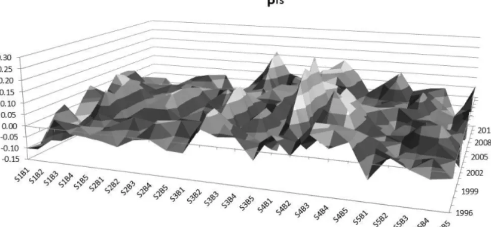
Table IV presents the full-sample beta estimates of the 25 global SBM portfolios relative to the excess returns of the AVG and long-short TS portfolios; the TS portfolio used in this regard is that of Table III, Panel D, row: 𝐸𝑊 (𝑅 = 1,3,6,12).18 High book-to-market and small stocks tend to have higher exposures to both commodity risk premia; however, these results may mask variations in betas over time which we allow for in our empirical procedure. The time-varying betas of the 25 global SBM portfolios and their t-ratios relative to the TS risk premium are presented in Figures 2 and 3 respectively; the variations are captured by rolling the regressions (1) and (2) forward using the procedure described in Section 2. We can see that both the betas and their t-ratios are stable over time for given portfolios and that the t-ratios present a slight tendency to increase over time.
< Insert Table IV and Figures 2 and 3 around here >
5. Robustness Checks and Additional Analysis
5.1. Sub-Sample Analysis
We repeat the analysis reported in Panels B to D of Table III over two consecutive sub-samples spanning January 1991 – December 1999 and January 2000 – December 2012, respectively.19
The choice of sub-samples is somewhat arbitrary but splits the overall data period available roughly in half. The risk premia associated with the backwardated and long-short TS portfolios for the sub-samples are mostly positive although the results for the early sub-sample are weaker
18 In order to preserve space, we do not present these estimates for all the regressors.
19 than for the whole sample. Likewise, the prices of risk associated with the contangoed portfolios are negative. For the most part, the magnitudes of the prices of commodity risk are similar to those reported in Table III. This indicates that investors persistently require rewards for holding stocks exposed to commodity risks. We note, however, a considerable reduction in the statistical significance of all prices of risk in the first sub-sample. We conjecture that this fall in statistical significance is at least in part a function of the fall in sample size from the regressions using the whole sample. This has obvious implications for the magnitudes of the standard errors that are inversely related to number of data points, all else equal.
Boons et al. (2014) argue that financialization led to lower participation costs and a reversal in signs of the premium earned on high-minus-low commodity beta stocks (from negative at -8% pre-2004 to positive at 11% post-2004). Their results are not directly comparable to ours because of differences in methodologies, base assets and commodity risks.20 However, this
notwithstanding, we also find much stronger evidence of a significant commodity risk premium in the second part of the sample.
5.2. Are the Commodity Risk Premia an Oil Risk Premium?
Crude oil makes up the majority of most weighted commodity index baskets. Increases in crude oil prices are also likely to have a more perilous impact on economic output, consumer price levels and firms’ profits than comparable rises in the prices of other less traded commodities such as frozen pork bellies. Hamilton (2009) provides a demonstration of the importance of oil for the economy through its effect on consumer purchasing power, arguing that oil price increases in
20 Our methodology differs from that of Boons et al. (2014) inasmuch as we use Fama and MacBeth (1973) two-step
approach to explain the pricing of size- and value-sorted global equity portfolios, when Boons et al. measure the difference in performance of equity portfolios sorted on commodity betas. Another key difference relates to the portfolios employed to proxy for commodity risks: we use AVG and TS when Boons et al. consider only one commodity portfolio which is similar in spirit to AVG.
20 2007-8 were a primary contributor to the ensuing recession even though the cause (increasing demand especially from China against a backdrop of flat supply) was fundamentally different to that of previous oil price spikes (which were primarily the result of significant supply interruptions). As a result, it is reasonable to question whether the observed premium which investors require for holding equities susceptible to commodity price changes is actually a noisy way to proxy for the impact of crude oil rather than that of a broader class of commodities.21 In
order to test this, we replicate the analysis reported in Table III but we now orthogonalize the excess returns of our commodity portfolios22 to the excess return of crude oil so that the former
are linearly purged of any influence coming from the latter. The results, reported in Table V, indicate that our main conclusions regarding the signs and statistical significances of the prices of
TS risk are fully robust to the exclusion of crude oil. We conclude therefore that the results reported thus far are not an artifact of crude oil.
< Insert Table V around here >
5.3. Financial and Macroeconomic Risk Factors
As discussed in Section 3, it may be that commodity price changes are merely capturing information that could be modeled more directly using macroeconomic variables, including most notably exposures to unexpected inflation. In order to test this, Table VI presents the averages of the prices of risk estimated from second-stage cross-sectional regressions that employ shocks to a set of financial and macroeconomic variables as risk factors. It is clear from the parameter estimates and their t-statistics that the key messages from the above analysis remain. The
21 Chen et al. (1986) originally test for, and find evidence against, an oil term being significant in pricing the
cross-section of equity returns. They surmise that the effect of oil price rises could be picked up more cleanly by other variables such as national output.
22 The orthogonalization is applied to AVG, to the backwardated, contangoed, and long-short portfolios based on the
21 estimated TS risk premia are of similar magnitude as in Table III, with unchanged levels of statistical significance for the long and long-short portfolios; the contangoed portfolios now attract negative and often statistically significant risk premia. Therefore, we conclude that the proposed commodity risks command premia in the cross-section of equity returns that are distinct from, and more important than, those obtained from exposure to inflationary or financial factors. Interestingly, among the financial and macroeconomic factors themselves, only changes in expected inflation are positively and significantly (at the 5% level) priced in the cross-section of the 25 global SBM portfolios; none of the other financial and macroeconomic risk premia is significant even at the 10% level. These conclusions hold irrespective of the statistic considered (Shanken’s t-statistic or bootstrap p-value).
< Insert Table VI around here >
5.4. Are AVG and TS Proxies for Future Economic Activity?
The motivation for a link between equity and commodity returns presented above presumes that rises in commodity prices are unambiguously negative due to the adverse impact that they will have on firm profitability and general economic inflation, with consequent reductions in consumer purchasing power.23 However, it has also been argued that commodity price rises may
be a positive signal of increasing economic activity in the future.24 It is also possible that the
23 This is the case of rises in crude oil prices that are deemed to contribute to a reduction of economic growth and
falling stock prices (Hamilton, 1983, 2009; Jones and Kaul, 1996; Driesprong et al., 2008).
24 Hu and Xiong (2013) argue that the positive correlation between commodity futures overnight returns and next
day East Asian stock price changes is indicative of the information-content of the former concerning world economic activity. Similarly, Bakshi, Panayotov and Skoulakis (2014) suggest that increases in the Baltic Dry Index might occur at the same time as rises in commodity and stock prices in anticipation of a subsequent increase in economic growth.
22 relationship between commodity prices and the business cycle is time-varying.25 There exists a
substantive and entirely separate literature that investigates the properties of certain time-series to predict future levels of industrial production several quarters ahead.26 Since these series are noisy
and their individual forecasting power may vary over time, a set of composite leading indicators, combining several individual leading series in a weighted fashion, are also constructed. The most commonly used such composite leading indicator (CLI) is the World CLI produced by the OECD.27
We rerun the two-step regression procedure, using all financial and macroeconomic indicators in Table VI discussed above alongside the monthly unexpected change in the OECD World CLI (UCLI) for the entire 1991-2012 sample period. The results for the lambda estimates are presented in Table VII. The risk premia for UCLI are not statistically significant even at the 10% level. Of particular interest to the present study is whether the coefficients on the AVG and
TS portfolios differ compared with the corresponding values reported in Table VI. There is clearly no reduction in the strength of the long, short and long-short risk premium based on TS. This suggests that the two commodity portfolios we propose (AVG and TS) are entirely separate sources of risk compared with that embodied in UCLI.
< Insert Table VII around here >
6. Conclusions
This article studies the pricing of two hypothesized commodity risks in the cross-section of equity returns. The first commodity risk is modelled as exposure to a long-only equally-weighted
25 Specifically focusing on industrial metals, Jacobsen et al. (2013) suggest that during recessions, a rise in
commodity prices is a positive signal of increasing subsequent economic activity, while the reverse is true during expansions when the level of activity is already high and further price rises are considered as signs of “overheating”.
26 See, for example, Bandholz and Funke (2003), Banerjee and Maellino (2006).
27The CLI series comprises: Dwellings started (number), Net new orders for durable goods (USD), Share prices:
NYSE composite (2010=100), Consumer sentiment indicator (normal = 100), Weekly hours of work: manufacturing (hours), Purchasing managers index (% balance), Spread of interest rates (% p.a.).
23 portfolio of commodity futures (AVG); the second commodity risk is measured as sensitivity to a long-short term structure portfolio (TS) that captures phases of backwardation and contango in commodity futures markets. Our motivation for studying this question comes from the ambiguous impact of commodity risk on stock returns. While they could signal worsening cost bases and reductions in profitability, rising commodity prices could also indicate improving expected growth in the real economy and thus potentially higher firm profitability. The question of the sign and statistical significance of the AVG and TS risk premia in the cross-section of equity returns thus needs to be tested empirically.
We present evidence that exposures to the TS of commodities command positive and statistically significant risk premia in the cross-section of the excess returns of the 25 global SBM equity portfolios of Fama and French (1998). The signs obtained on the risk premia indicate that investors perceive periods of expected rising commodity prices as bad news; they then demand compensation for exposure to commodity price risk. Vice versa, periods of expected falling commodity prices are perceived as good news; investors are then happy to earn lower expected returns on equities that are sensitive to commodity price risks. Further evidence suggests that the conclusions are not an artifact of crude oil. They are also robust to the analysis of sub-samples and to several specifications of the asset pricing model employed such as those developed by Carhart (1997) or Chen et al. (1986).
While our research presents a clear demonstration that commodity risks are priced in global financial markets, an obvious question for future research is why this is the case. Commodity and stock prices are linked, both directly and indirectly, as a result of the important use of commodities in production processes. The direct effect of commodity price rises occurs when changes in the cost of commodities affect a firm’s profitability where commodities are a significant proportion of their overall costs. The indirect impact takes place through their effects
24 on the inflation rate via the costs of goods, and the resulting fall in consumers’ purchasing power will then adversely affect their demand for end products and services. Eventually, this feeds through to firms’ cash-flows (see Jones and Kaul, 1996). It would be of interest to investigate which of these two channels is the more prominent in driving commodity risk premia.
Acknowledgements
The authors are grateful to two anonymous referees and the Editor, Nathan Joseph, for useful comments on a previous version of the paper.
25
REFERENCES
Acharya, V., Lochstoer, L. and Ramadorai, T. (2013). Limits to arbitrage and hedging: Evidence from commodity markets. Journal of Financial Economics, 109, 441–465.
Bakshi, G., Gao, X., and Rossi, A. (2015) Understanding the sources of risk underlying the cross-section of commodity returns, Unpublished Working Paper, University of Maryland.
Bakshi, G., Panayotov, G. and Skoulakis, G. (2014). The Baltic dry index as a predictor of global stock returns, commodity returns and global economic activity. Working paper, Smith School of Business, University of Maryland.
Bandholz, H. and Funke, H. (2003). In search of leading indicators of economic activity in Germany. Journal of Forecasting, 22, 277–297.
Banerjee, A. and Marcellino, M. (2006). Are there any reliable leading indicators for US Inflation and GDP growth? International Journal of Forecasting, 22, 137–151.
Basu, D. and Miffre, J. (2013). Capturing the risk premium of commodity futures: The role of hedging pressure. Journal of Banking and Finance, 37, 2652–2664.
Bessembinder, H. (1992). Systematic risk, hedging pressure, and risk premia in futures markets. Review of Financial Studies, 5, 637–667.
Bodnar, G.M., Hayt, G.S. and Marston, R.C. (1998). Wharton survey of financial risk management by US non–financial firms. Financial Management 27(4), 70–91.
Boons, M., de Roon, F. and Szymanowska, M. (2014). The price of commodity risk in stock and futures markets. Working paper, Nova School of Business and Economics.
Brennan, M. (1958). The supply of storage. American Economic Review, 48, 50–72.
Carhart, M.M. (1997). On persistence in mutual fund performance. Journal of Finance, 52, 57– 82.
Chen, N–F., Roll, R. and Ross, S.A. (1986). Economic forces and the stock market. Journal of Business, 59, 383–403.
Cochrane, J.H. (1996). A cross–sectional test of an investment–based asset pricing model. Journal of Political Economy, 104, 572–621.
Cochrane, J.H. (2001). A rehabilitation of the stochastic discount factor methodology. Working paper, University of Chicago.
Cochrane, J.H. (2005). Asset Pricing. Princeton University Press, Princeton, NJ.
Cootner, P. (1960). Returns to speculators: Telser vs. Keynes. Journal of Political Economy, 68, 396–404.
26 Daskalaki, C., Kostakis, A., and Skiadopoulos, G. (2014). Are there common factors in
commodity futures returns?. Journal of Banking and Finance, 40(3), 346–363.
Dewally, M., Ederington, L. and Fernando, C. (2013). Determinants of trader profits in commodity futures markets. Review of Financial Studies, 26, 2648–2683.
Driesprong, G., Jacobsen, B. and Maat, B. (2008). Striking oil: Another puzzle. Journal of Financial Economics, 89, 307–327.
El-Masry, A.A. (2006). Derivatives use and risk management practices by UK nonfinancial companies. Managerial Finance, 32(2), 137–159.
Erb, C. and Harvey, C. (2006). The strategic and tactical value of commodity futures. Financial Analysts Journal, 62, 69–97.
Fama, E. and French, K. (1987). Commodity futures prices: Some evidence on forecast power, premiums, and the theory of storage. Journal of Business, 60, 55–73.
Fama, E. F. and French, K.R. (1993). Common risk factors in the returns on stocks and bonds.Journal of Financial Economics, 3, 3–56.
Fama, E. F. and French, K.R. (1998). Common risk factors in the returns on stocks and bonds. Journal of Finance, 53, 1975–1999.
Fama, E. F. and MacBeth, J. D. (1973). Risk, returns, and equilibrium: Empirical tests. Journal of Political Economy, 81, 607–636.
Gorton, G., Hayashi, F. and Rouwenhorst, G. (2013). The fundamentals of commodity futures returns. Review of Finance, 17, 35–105.
Gorton, G. and Rouwenhorst, G. (2006). Facts and fantasies about commodity futures. Financial Analysts Journal, 62, 47–68.
Hamilton, J.D. (1983). Oil and the macroeconomy since World War II. Journal of Political Economy, 91, 228–248.
Hamilton, J.D. (2009). Causes and consequences of the oil shock of 2007–08. Brookings Papers on Economic Activity, Spring, 215–283.
Hansen, L.P. (1982). Large sample properties of generalized method of moments estimators. Econometrica 50(4), 1029–1054.
Haushalter, G.D. (2000). Financing policy basis, risk, and corporate hedging: Evidence from oil and gas producers. Journal of Finance, 55, 107–152.
Hirshleifer, D. (1988). Residual risk, trading costs, and commodity futures risk premia. Review of Financial Studies, 1, 173–193.
27 Hong, H. and Yogo, M. (2012). What does futures market interest tell us about the
macroeconomy and asset prices? Journal of Financial Economics, 105, 473–490.
Hou, K. and Szymanowska, M. (2013). Commodity–based consumption tracking portfolio and the cross–section of average stock returns. Working Paper, Rotterdam School of Management, Erasmus University.
Hu, C. and Xiong, W. (2013). Are commodity futures prices barometers of the global economy. In Après le Deluge: Finance and the Common Good after the Crisis, E.G. Weyl, E.L. Glaeser and T. Santos, eds. University of Chicago Press, forthcoming.
Jacobsen, B., Marshall, B.R. and Visaltanachoti, N. (2013). Stock market predictability and industrial metal returns. Working Paper, School of Economics and Finance, Massey University.
Jin, Y. and Jorion, P. (2006). Firm value and hedging: evidence from oil and gas producers. Journal of Finance, 61(2), 893–918.
Jones, C.M. and Kaul, G. (1996). Oil and the stock markets. Journal of Finance, 51, 463–491. Kaldor, N. (1939). Speculation and economic stability. Review of Economic Studies,7, 1–27. Kan, R. and Zhou, G. (1999). A critique of the stochastic discount factor methodology. Journal of
Finance 54(4), 1221–1248.
Kosowski, R., Timmerman, A., Wermers, R. and White, H. (2006). Can mutual fund “stars” really pick stocks? New evidence from a bootstrap analysis. Journal of Finance, 61(6), 2551– 2595.
Lo, A. W. (2002). The Statistics of Sharpe Ratios. Financial Analysts Journal, 58(4), 36–52. Miffre, J., Fuertes, A–M. and Fernandez–Perez, A. (2015). Commodity markets, long-horizon
predictability and intertemporal pricing. Review of Finance, forthcoming.
Newey, W. K., West, K. D., (1987). Hypothesis testing with efficient method of moments estimation. International Economic Review 28, 777-787.
Orbendorfer, U. (2009). Energy prices, volatility and the stock market: Evidence from the Eurozone. Energy Policy, 37, 5787–5795.
Panaretou, A. (2014) Corporate risk management and firm value: evidence from the UK market. European Journal of Finance, 20(12), 1161–1186.
Ross (1976). The arbitrage theory of capital asset pricing. Journal of Economic Theory, 13(3), 341–360.
Shanken, J. (1992). On the estimation of beta–pricing models. Review of Financial Studies, 5, 1– 33.
28 Szymanowska, M., de Roon, F., Nijman, T. and Van Den Goorbergh, R. (2014). An anatomy of
commodity futures risk premia. Journal of Finance, 69, 453–482.
29 Figure 1: 45 Degree Line for Commodity versus non-Commodity Models
30 Figure 2: Surface Plot for Rolling Betas on the Term Structure Portfolio
36 Table I. Summary statistics for the excess returns of long backwardated, short contangoed and long-short commodity portfolios
The table shows summary statistics for the monthly returns of long, short and long-short commodity portfolios. The three sets of columns headed ‘Long backwardation’, ‘Short contango’, and ‘Long-short portfolio’ refer to the three different approaches to forming the commodity portfolios by taking the 25% of most backwardated or/and most contangoed commodities. The sorting criterion in Panel A (Panel B) is the roll-yields (hedging pressure of hedgers and speculators) averaged over the previous R months with R= 1, 3, 6 and 12 months. EW (R=1, 3, 6, 12) stands for the excess returns of a portfolio that equally weights and monthly rebalances the backwardated (contangoed and long-short, respectively) portfolios with the four different horizons. Mean and SD stand for annualized mean excess returns and annualized standard deviation of excess returns, respectively; Sharpe equals Mean/SD, Lo’s (2002) t-statistics are in parentheses. Estimation period: January 1991-December 2012. SD Sharpe t -Sharpe t - SD Sharpe t -Sharpe SD Sharpe t -Sharpe t
-Panel A: Sorting based on the slope of the term structure
R=1 0.0184 (0.44) 0.1946 0.0948 (0.44) -0.0670 (-1.89) 0.1665 -0.4023 (-1.88) 0.0427 (1.89) 0.1059 0.4031 (1.88) R=3 0.0909 (2.48) 0.1717 0.5294 (2.47) -0.0812 (-2.45) 0.1554 -0.5227 (-2.44) 0.0861 (4.64) 0.0869 0.9903 (4.55) R=6 0.0711 (1.98) 0.1682 0.4228 (1.98) -0.0704 (-2.15) 0.1534 -0.4589 (-2.14) 0.0708 (3.61) 0.0919 0.7697 (3.57) R=12 0.0312 (0.83) 0.1758 0.1775 (0.83) -0.0456 (-1.38) 0.1554 -0.2932 (-1.37) 0.0384 (1.97) 0.0916 0.4192 (1.96) EW (R=1, 3, 6, 12) 0.0529 (1.52) 0.1637 0.3232 (1.51) -0.0660 (-2.10) 0.1472 -0.4485 (-2.09) 0.0595 (3.42) 0.0817 0.7283 (3.38)
Panel B: Sorting based on the hedging pressure of hedgers and speculators
R=1 0.0369 (1.04) 0.1661 0.2223 (1.04) -0.0398 (-1.22) 0.1526 -0.2606 (-1.22) 0.0383 (2.18) 0.0823 0.4657 (2.17) R=3 0.0134 (0.38) 0.1653 0.0812 (0.38) -0.0361 (-1.12) 0.1517 -0.2379 (-1.11) 0.0248 (1.47) 0.0789 0.3137 (1.47) R=6 0.0298 (0.90) 0.1550 0.1921 (0.90) -0.0446 (-1.30) 0.1611 -0.2771 (-1.30) 0.0372 (2.05) 0.0850 0.4377 (2.04) R=12 0.0607 (1.74) 0.1632 0.3717 (1.74) -0.0783 (-2.29) 0.1603 -0.4885 (-2.28) 0.0695 (3.96) 0.0823 0.8441 (3.90) EW (R=1, 3, 6, 12) 0.0352 (1.07) 0.1548 0.2273 (1.07) -0.0497 (-1.58) 0.1479 -0.3359 (-1.57) 0.0424 (2.72) 0.0733 0.5790 (2.70) Long-short portfolio
Mean Mean Mean
Short contango Long backwardation
37 Table II. Correlations between traditional and commodity risk factors
The table presents correlations between the excess returns of equally-weighted (AVG), backwardated, contangoed and long-short commodity portfolios on the one hand and the excess returns of various traditional risk premia on the other hand. The AVG portfolio is an equally-weighted monthly-rebalanced portfolio that is long all 27 commodities. The backwardated, contangoed and long-short portfolios are formed by taking the 25% most backwardated or/and most contangoed commodities based on roll-yields in Panel A (based on the positions of hedgers and speculators in Panel B) averaged over the previous R months. EW (R=1, 3, 6, 12) stands for the excess returns of a portfolio that equally weights and monthly rebalances the backwardated (contangoed and long-short, respectively) portfolios with R= 1, 3, 6 and 12 months. ERM, SMB, HML, and UMD are global market, size, value, and momentum risk premia. ***, ** and * indicate statistical significance at the 1%, 5% and 10% levels, respectively. Estimation period: January 1991-December 2012.
Panel A: Sorting based on the slope of the term structure (TS)
AVG 0.77 *** 0.76 *** 0.74 *** 0.78 *** 0.82 *** 0.75 *** 0.76 *** 0.74 *** 0.72 *** 0.79 *** 0.13 * 0.07 0.06 0.14 ** 0.12 * ERM 0.46 *** 0.30 *** 0.33 *** 0.38 *** 0.41 *** 0.38 *** 0.35 *** 0.34 *** 0.35 *** 0.33 *** 0.37 *** 0.00 0.02 0.05 0.11 * 0.05 SMB 0.14 ** 0.21 *** 0.17 ** 0.14 ** 0.11 * 0.17 ** 0.02 0.01 0.05 -0.01 0.02 0.19 *** 0.16 ** 0.08 0.11 * 0.15 ** HML -0.04 -0.08 -0.08 -0.13 ** -0.02 -0.08 -0.13 * -0.06 -0.07 0.00 -0.07 0.03 -0.02 -0.06 -0.02 -0.02 UMD -0.04 0.09 * 0.08 0.00 -0.02 0.04 -0.12 ** -0.12 ** -0.17 ** -0.15 ** -0.15 ** 0.19 *** 0.19 *** 0.14 ** 0.11 * 0.18 *** HP 0.64 *** 0.66 *** 0.65 *** 0.69 *** 0.74 *** 0.60 *** 0.60 *** 0.60 *** 0.60 *** 0.68 *** 0.13 ** 0.11 * 0.15 ** 0.18 *** 0.19 ***
Panel B: Sorting based on the hedging pressure of hedgers and speculators (HP)
AVG 0.81 *** 0.81 *** 0.80 *** 0.82 *** 0.85 *** 0.74 *** 0.76 *** 0.76 *** 0.76 *** 0.80 *** 0.14 0.11 * 0.01 0.07 0.09 ERM 0.46 *** 0.42 *** 0.40 *** 0.42 *** 0.37 *** 0.42 *** 0.37 *** 0.37 *** 0.39 *** 0.30 *** 0.38 *** 0.08 0.07 0.02 0.07 0.07 SMB 0.14 ** 0.13 ** 0.17 ** 0.19 *** 0.19 *** 0.18 *** 0.08 0.05 0.04 0.05 0.06 0.05 0.13 ** 0.13 ** 0.15 ** 0.13 ** HML -0.04 -0.04 -0.06 -0.08 -0.06 -0.06 -0.01 0.01 0.04 0.05 0.02 -0.03 -0.07 -0.11 * -0.10 * -0.09 UMD -0.04 -0.01 0.01 -0.03 -0.01 -0.01 -0.08 -0.08 -0.06 -0.04 -0.07 0.06 0.09 0.03 0.03 0.06 TS 0.64 *** 0.66 *** 0.65 *** 0.69 *** 0.74 *** 0.60 *** 0.60 *** 0.60 *** 0.60 *** 0.68 *** 0.13 ** 0.11 * 0.15 ** 0.18 *** 0.19 *** R=1 EW (R=1, 3, 6, 12) R=1 Panel I: AVG
Panel III: Short contango Panel II: Long backwardation
R=1
Panel IV: Long-short portfolio
R=3 R=6 R=12 R=12 EW (R=1, 3, 6, 12) EW (R=1, 3, 6, 12) R=3 R=6 R=12 R=3 R=6