Optimizing Liquidity Usage and Settlement Speed in Payment Systems

BANK OF FINLAND

DISCUSSION PAPERS

16/99

Harry Leinonen – Kimmo Soramäki

Financial Markets Department 12.11.1999

Optimizing Liquidity Usage and

Settlement Speed in Payment Systems

BANK OF FINLAND DISCUSSION PAPERS 16/99

Harry Leinonen – Kimmo Soramäki

Financial Markets Department 12.11.1999

Optimizing Liquidity Usage and

Settlement Speed in Payment Systems

The views expressed here are those of the authors and do not necessarily correspond those of the Bank of Finland.

ISBN 951-686-636-0 ISSN 0785-3572

Suomen Pankin monistuskeskus Helsinki 1999

Optimizing Liquidity Usage and Settlement Speed

in Payment Systems

Bank of Finland Discussion Papers 16/99

Harry Leinonen – Kimmo Soramäki

Financial Markets Department

Abstract

The operating speed of a payment system depends on the stage of technology of the system’s communication and information processing environment. Frequent intraday processing cycles and real-time processing have introduced new means of speeding up the processing and settlement of payments. In a real-time envi-ronment banks face new challenges in liquidity management. They need to plan for intraday as well as interday fluctuations in liquidity. By employing various types of hybrid settlement structures, banks may be able to even out intraday fluctuations in liquidity demand. The aim of this study is to develop a framework for analysing fluctuations in liquidity demand and assessing the efficiency of dif-ferent settlement systems in terms of speed and liquidity needs.

In this study we quantify the relationship between liquidity usage and set-tlement delay in net setset-tlement systems, real-time gross setset-tlement systems and hybrid systems, as well as the combined costs of liquidity and delay in these sys-tems. We analyse ways of reducing costs via optimization features such as netting of queues, offsetting of payments and splitting of payments. We employ a pay-ment system simulator developed at the Bank of Finland, which enables us to evaluate the impact of changes in system parameters and thus to compare the ef-fects of alternative settlement schemes with given payment flows. The data used covers 100 days of actual payments processed in the Finnish BoF-RTGS system.

Our major findings relate to risk reduction via real-time settlement, effects of optimization routines in hybrid systems, and the effects of liquidity costs on banks’ choice of settlement speed. A system where settlement takes place con-tinuously in real-time and with queuing features is more efficient from the per-spective of liquidity and risks than a net settlement system with batch processing. Real-time processing enables a reduction in payment delay and risks without nec-essarily increasing liquidity needs. Participants will operate under immediate payment/settlement if liquidity costs are low enough relative to delay costs and if the liquidity arrangements are sufficiently flexible. The central bank can therefore support risk reduction and payment speed objectives by providing low cost intra-day liquidity as well as more flexible ways for participants to add or withdraw liquidity from the system. Optimizing and gridlock solving features were found to be effective at very low levels of liquidity. The efficiency of the different optimi-zation methods for settlement systems are affected by the actual flow of payments processed. Gains from netting schemes with multiple daily netting cycles were found to be somewhat more limited.

Likviditeetin ja selvitysnopeuden optimointi

maksujärjestelmissä

Suomen Pankin keskustelualoitteita 16/99

Harry Leinonen – Kimmo Soramäki

Rahoitusmarkkinaosasto

Tiivistelmä

Maksujärjestelmien toimintanopeus riippuu järjestelmän tiedonvälityksen ja -käsit-telyn teknisestä tasosta. Lukuisat päivänsisäiset käsittelykerrat ja reaaliaikaiset jär-jestelmät ovat mahdollistaneet maksujen aiempaa nopeamman välityksen ja sel-vityksen. Reaaliaikaisessa ympäristössä pankkien likviditeetinhallintaan kohdistuu uusia haasteita, kun päivänsisäisen suunnitteluperiodin merkitys on kasvanut päiväkohtaisen suunnittelun lisäksi. Erilaisilla hybridi-järjestelmillä päivänsisäisen likviditeetintarpeen vaihteluita voidaan tasoittaa. Tämän tutkimuksen tavoitteena on luoda kehikko likviditeetin vaihteluiden analysointia ja erilaisten maksujärjestel-mien likviditeettiä ja toimintanopeutta parantavien menetelmaksujärjestel-mien arviointia varten

Tutkimuksessa arvioidaan likviditeetin käytön ja selvitysviipeen suhdetta nettoselvitysjärjestelmissä, reaaliaikaisissa bruttoselvitysjärjestelmissä ja hybridi-järjestelmissä sekä myöskin likviditeetin ja viipeen yhteiskustannuksia näissä. Kus-tannusten pienentämistä tutkitaan erilaisten optimointimenetelmien, kuten jonotta-vien maksujen nettoutuksen, vastakkaisten maksujen kumoamisen ja maksujen pilk-komisen avulla. Tutkimuksessa käytetään Suomen Pankissa kehitettyä maksu-jär-jestelmäsimulaattoria, joka mahdollistaa järjestelmäteknisten muutosten ja erilaisten selvitystapojen vaikutusten arvioinnin samaa maksuaineistoa käyttäen. Mak-suaineistona käytetään 100 päivän aikana Suomen Pankin sekkitilijärjestelmässä suoritettuja maksuja.

Tutkimuksen päätulokset liittyvät reaaliaikaisen selvityksen tuomaan riskien pienentämiseen, optimointimenetelmien vaikutuksiin hybridijärjestelmissä ja suh-teellisten likviditeettikustannusten vaikutukseen pankkien käyttäytymisessä. Reaali-aikainen ja jatkuva selvitysjärjestelmä, jossa on käytössä jonotusmekanismi, on likviditeetin ja riskien näkökulmasta tehokkaampi kuin eräpohjaiset nettoselvi-tysjärjestelmät. Reaaliaikaisuudella voidaan vähentää viivettä maksujen lopullisessa selvityksessä ja järjestelmän riskipitoisuudessa ilman että likviditeetintarve kasvaa. Järjestelmän osallistujat toimivat ilman selvitysviivettä, mikäli likviditeetti-kustannukset ovat tarpeeksi pienet viivekustannuksiin verrattuna. Joustavammat likviditeettijärjestelyt alentavat likviditeetin kustannuksia. Keskuspankit voivat vähentää maksujärjestelmän riskejä ja nopeuttaa maksujen selvitystä tarjoamalla edullista päivänsisäistä likviditeettiä ja järjestämällä osallistujille entistä joustavam-pia tapoja lisätä ja vetää pois likviditeettiä järjestelmästä. Likviditeetin optimointi-menetelmät ja järjestelmän lukkiutumistilanteiden (gridlock) syntymistä estävät ja purkavat ominaisuudet havaittiin tehokkaammiksi, mikäli osallistujilla oli vain vähän likviditeettiä käytössä. Päivänsisäisten nettoutuskertojen lisäämisestä koitu-vat edut havaittiin nettojärjestelmien kannalta vähäisiksi.

Contents

Abstract 5

Tiivistelmä 6

1 Introduction 9

2 Interbank payment settlement designs 10 3 Previous research on payment systems 12

4 Simulation framework 14

4.1 Payment and settlement delay 14

4.2 Concepts of liquidity 14

4.3 Cost components in settlement systems 16 4.4 The payment systems simulator 17 4.5 Simulated settlement systems 18

4.6 Data 20

5 Simulations results 22

5.1 Relationship between liquidity usage and settlement delay 22 5.2 Combined cost of liquidity and delay 23 5.3 Gridlocks in RTGS systems 26 5.4 Optimizing an RTGS system 28 6 Applicability of the findings and some conclusions 31

References 33

1

Introduction

The operating speed of a payment system has always depended on the stage of technology of the system’s communication and information processing environ-ment. The use of information technology in batch processing has enabled a reduc-tion in payment processing time from several days in the forgone manual era to typically one day. Frequent intraday processing cycles, and especially real-time processing, have introduced new means of further speeding up payment process-ing and settlement. With increasprocess-ing payment volumes, there is now a need to reas-sess risk management in existing payment settlement systems. One way to reduce interbank settlement risks is to speed up the settlement process.

In a real-time environment banks face new challenges in liquidity manage-ment. They need to plan for intraday as well as interday fluctuations in liquidity. Not all payments in a real-time environment require immediate processing. This gives system participants the opportunity to employ different types of hybrid set-tlement structures, which enables the evening out of intraday fluctuations in li-quidity demand. The aim of this study is to develop a framework for analysing fluctuations in liquidity demand and assessing the efficiency of different settle-ment systems, particularly from the viewpoint of liquidity and settlesettle-ment speed.

In this study we try to determine system-level cost-optimal liquidity usage for various settlement systems and compare the systems as they operate with op-timal amounts of liquidity. We quantify the relationship between liquidity usage and settlement delay in net settlement systems, real-time gross settlement systems and hybrid systems, as well as the combined costs of liquidity and delay in these systems. We analyse ways of reducing costs via optimization features such as netting of queues, offsetting of payments and splitting of payments. Whether the system-level cost-optimum is reached through independent decisions of system participants is not discussed here. Our major findings relate to risk reduction via real-time settlement, effects of optimization routines in hybrid systems, and the effects of liquidity costs on banks’ choice of settlement speed. Whether the opti-mal settlement mode is real-time or delayed depends on the cost relationships between these factors. The study focuses on the optimization of settlement proc-esses under normal operating conditions. Exceptional situations relating to par-ticipant failures and general system crises are beyond the scope of the analysis. However, the risk reduction measures studied would also be helpful in these kinds of exceptional situations.

In the empirical part of our study, we employ a payment system simulator developed at the Bank of Finland. The simulator enables us to evaluate the impact of changes in system parameters and thus to compare the effects of alternative settlement schemes with given payment flows. The random and structural char-acteristics of payment flows have major effects on the results. A payment sys-tem’s liquidity need, assuming a given processing speed, is determined by the payment flows and by the specific settlement structure. The study is organized as follows. The next two sections provide a brief overview of alternative settlement designs and a summary of related research. In section 4, the terminology, methods and data are described. In section 5, we present our results concerning settlement speed, liquidity usage, risk and cost components as well as gridlock issues and optimization possibilities. Section 6 concludes with a summary of the key findings and a discussion of related limitations and applicability.

2

Interbank payment settlement designs

A major distinction between different interbank payment systems is whether a system is operating on a net or gross basis and whether payments are processed individually or in batches. The most common three pure implementations of these principles are real-time gross settlement, time-designated net settlement and con-tinuous or secured net settlement. Systems combining net and gross settlement or individual and batch processing are often referred to as hybrid systems.

A pure real-time gross settlement (RTGS) system is defined as a system in which, for each transaction, delivery of payment information and final settlement in central bank money take place simultaneously and continuously. Transfers are settled individually during the day without netting debits against credits. An RTGS system provides continuous intraday finality for the processed transfers (BIS 1997). In a time-designated net settlement (TDNS) system, the settlement of payments occurs on a net basis at predefined points of time during the day or at the end of the day. The net position, ie the sum of payments the bank has received up to the end of the settlement period minus the payments it has sent, can either be calculated on a bilateral or multilateral basis. Although many G10 countries have introduced real-time gross settlement systems, according to Folkerts-Landau et al (1996) most of the payment volume in the industrialized countries is settled by multilateral netting.

After the interbank payment transfer is initiated and the customer’s account debited, the settlement process is generally separated into two sub-processes: final customer crediting and final interbank settlement. Except in pure RTGS systems, the payment information and settlement are processed in separate systems and there is a need for synchronization at certain points of time. A counterparty or settlement risk will arise if the customer payment becomes final before the inter-bank settlement. In such case, settlement of the payment is delayed and the coun-terparty risk will include the total or net amount of outstanding delayed settle-ments, depending on the legal rules for netting claims. In order to reduce the risk, the receiving bank can delay payment to the customer. When this is the general practice, final settlements are processed simultaneously or prior to final crediting of the customer. In a system with rapid payment information processing, this will entail the delay payments in order to allow the slower settlement process to catch up with the payment process. With the same payment flows and settlement times, the amount of delayed payments in a system without settlement risk will equal the total settlement delays in a system with settlement risk. We will refer to settlement delay and payment delay respectively in distinguishing between systems with and without settlement risk.

In continuous net settlement (CNS) systems, payments are credited indi-vidually and immediately to receivers’ accounts, but final settlements occur peri-odically or at the end of the day. These systems entail settlement delay, and the amount of risk depends on the total or net value of delayed settlements. To control the risks, participants usually have credit limits, which may be partly or com-pletely collateralized. An RTGS system with queuing arrangements operating with central bank money is analytically equivalent to a secured CNS system (SNS) with fully collateralized debt limits. In both designs, payments are credited to the receiver’s accounts only if there are sufficient covering funds or collateral. If the bank does not have sufficient liquidity to settle the payment, the payment is delayed and credited to the customer’s account only after settlement. When we

refer later to a CNS system, we will assume that it entails counterparty risk, ie that settlements are delayed.

Hybrid settlement systems try to combine elements from several of the above systems in order to achieve better performance than with pure systems. Hy-brid systems are designed to optimize with respect to the different settlement de-lay and liquidity costs associated with the pure systems. An RTGS system with queuing, for example, can be considered a hybrid system.

3

Previous research on payment systems

Previous research on payment systems is generally policy oriented, much of it being conducted by central banks around the world, mainly in Italy, the United Kingdom and the United States. Most of the research on payment settlement sys-tems can be included in one of the following three categories: descriptions of cur-rent arrangements, analysis of the risks associated in these systems and central bank policy issues and comparisons of net and gross settlement systems.

The settlement systems in use in different countries have evolved for the most part independently of each other. Until recently there has been little effort to harmonize or standardize these systems. The first category consists of studies that attempt to describe systems in use in different countries. The goal has been to find a common structure and the key similarities and differences among these systems. The study by Borio, Russo and Bergh (1992) provides an overview of the com-mon structure underlying different settlement systems. Another earlier study is the survey by the Committee on Payment and Settlement Systems (CPSS) 1 on large-value funds transfer systems in the G10 countries (BIS 1990). The report by CPSS on Real-time gross settlement (BIS 1997) is a good review of the concepts relat-ing to RTGS systems.

BIS (1989), Borio and Van den Bergh (1993) and Angelini et al (1996) pro-vide good analyses of issues concerning systemic risk in payment systems, the emphasis being on netting systems. From the viewpoint of this study, the most interesting papers are those on systemic risk that simulate situations in which one or more system participants fail to settle their obligations. The data used in Hum-phrey (1986) are from the Clearinghouse Interbank Payment System (CHIPS)2. McAndrews and Wasilyew (1995) build on Humphrey (1986) and use generated data to study factors that affect the systemic risk in a payment system. In Kuus-saari (1996) the extent and effects of a systemic crisis in Finland are analysed em-pirically by using simulated bank failures. These studies use the same methodol-ogy, ie they use ex post settlement data to assess the impacts of bank failures on other system participants. The simulation model used in this study differs from the model used in those studies in that it simulates the operation of a settlement sys-tem rather than specific events occurring in a syssys-tem. In our simulations, a bank may fail to settle, but this would be a simulation output rather than input.

The central bank policy issues studied include inter alia the central bank’s intraday credit policy (eg Humphrey 1990, Furfine and Stehm 1997), the possible emergence of private intraday money markets (Rossi 1995), and the effects of these on monetary policy (Dale and Rossi 1996). The issue of externalities in payment systems, ie third party effects not internalized in the payment system (eg the effects of payment delays), have been studied by Schoenmaker (1993). The studies by Angelini (1998) and Kahn and Roberds (1998b) also deal with exter-nalities; these studies analyse the effects on banks’ settlement behaviour of insuf-ficient or costly liquidity in an RTGS system. The common goal of this research has been to find methods by which the central bank can ensure the stability and smooth functioning of the payment system.

1

The Committee on Payment and Settlement Systems (CPSS) is a working group under the Bank for International Settlement (BIS). It was established by the governors of the central banks of the G10 countries to monitor and analyse developments in payment and settlement systems.

2

CHIPS is an interbank settlement and payment transfer system organized by the New York Clearing House Association, a group of the largest banks in the city.

The third body of literature comprises studies that compare the efficiency of net settlement and real-time gross settlement systems. However, efficiency com-parisons between different implementations of net or real-time gross settlement systems with queuing facilities are rare. These studies are generally analytical. Schoenmaker (1995) uses an analytical model to compare pure RTGS systems with net settlement systems with caps and loss sharing rules. Kahn and Roberds (1998a) compare the merits of net and gross systems in a framework of bank in-centives and moral hazard problems. Kobayakawa (1997) probes whether there is a rationale for gross and net settlement systems to coexist in the same economy. A recent study by Freixas and Parigi (1998) analyses the tradeoff between risks and efficiency in net and gross settlement.

Simulations that compare and quantify the efficiency of different imple-mentations of real-time gross settlement systems or net settlement systems have been very rare, perhaps due to data security issues and the demanding processing requirements of simulations. However, some studies have been done. Günzter et al (1997) present several heuristic algorithms for bilateral and multilateral netting of payments in reference to the German payment settlement system Elektronische Abrechnung mit Filetransfer 2 (EAF-2)3. Ganz et al (1998) simulate the efficiency of these algorithms in securities settlement. An earlier study by Boeschoten (1989) uses simulations to assess the impacts of different queuing mechanisms on the Dutch interbank payment system, which operates on the basis of real-time gross settlement. Non-academic simulation exercises in the planning phase of a new system or in assessing the efficiency of existing systems have been done in several countries. The Swiss National Bank has used simulations in assessing the queuing mechanism in SIC4 (Vital and Mengle 1988, Vital 1990 and 1994), the Association for Payment Clearing Services (APACS)5 in refining the CHAPS6 system (Bowman 1995), and recently the Banque de France in introducing its new RTGS system. For the Continuous Linked Settlement (CLS) system, which will be operational in mid-2000, simulations have been run with different settlement volumes in order to assess its operational capacity and the planned paying sched-ules.

3

The Elektronishce Abrechnung mit Filetransfer 2 (EAF-2, currently Euro Access Frankfurt) is the largest interbank settlement system in Germany and is operated by the Hessian branch of the Bundesbank.

4

SIC (Swiss Interbank Clearing) is a payment settlement system operated by Telekurs SIC AG under the authority of the Swiss national Bank (SNB).

5

APACS (Association for Payment Clearing Services) is the industry body for the UK’s major banks and building societies and has 29 members. It oversees money transmission and has respon-sibility for the co-operative aspects of the UK payments industry.

4

Simulation framework

4.1

Payment and settlement delay

The unit of analysis in this study is a settlement system comprising banks and non-bank entities, which are referred to system participants. The participants are continuously sending and receiving payments during the day, and the settlement of these payments is recorded, according to established settlement rules, in the settlement accounts.

In this study, the payment or settlement delay for each payment is calculated as the time difference between payment origination by the sending bank and final and irrevocable settlement of the payment. The cost of delay is likely to depend on the value of the delayed payment as well as the duration of the delay. The de-lay indicator, ρ, is calculated as the ratio of the cumulative sum of payments that have entered the system but remain unsettled (4) to the absolute cumulative value of outgoing payments (₉2_{) up the end of the day:}

∑

∑

If all payments are settled immediately upon entry into the system, ρ = 0; if all payments are delayed until the end of the day, ρ = 1. A possible interpretation of the indicator would be the share of payments that are settled at the end of the day instead of immediately.

4.2

Concepts of liquidity

In modern payment systems where payments are processed in real-time or in batches during the day, liquidity not only has end-of-day value but also intraday value. We analyse a settlement period of one day, during which the liquidity available to the participants is either employed for settlement purposes or remains idle on participants’ settlement accounts. The amount of liquidity being employed by a participant, /H, at a moment W when payments are settled immediately upon entry to the system depends on the flow of incoming and outgoing payments. The amount of liquidity employed at any moment in the day equals the excess cumu-lative value of outgoing payments, VO, as compared to incoming payments, VI at each point of time W:

7 W 9 9 / W L W L 2 L , L H W min(0, ) , 0,1,2,..., 0 0 = − =

∑

∑

One of the main decision variables in the study is the amount of liquidity available to the participants initially at the start of the day, for which we use the theoretical bounds of liquidity as calculated in Koponen and Soramäki (1998). To calculate these bounds, it is assumed that the external liquidity source for any participant

during the day is limited to its initial liquidity, ie the initial balance on its central bank settlement account and a possible intraday overdraft. Because the delaying of payments and settlements are analytically equivalent in this context, we use payment delay to describe both situations where payments are delayed to allow the settlement process to catch up and situations where only the final settlements are delayed. If account holders are required only to have sufficient funds at the end of the day (W 7 ), they can delay their payments until the end of the day and need only enough liquidity to cover the net amount of all incoming and outgoing payments at the end of the day, ie the lower bound (//) of liquidity:

H 7 / _/

/ = (3)

If during the day sufficient liquidity is not available, payments are delayed. At the lower bound of liquidity, payment delay is at its maximum and any reduction in liquidity would mean a failure to settle one or more payments during the day. The liquidity need for an end-of-day net settlement system equals the lower bound of liquidity. In fact, the lower bound of liquidity marks the minimum external li-quidity needed in all settlement systems where payments can be delayed eg by queuing, whether operating on a net or gross basis.

The upper bound (/8) of liquidity equals the amount of liquidity that must be available to the participants for immediate settlement throughout the day. Any additional liquidity above the upper bound remains idle on participants’ settlement accounts for the whole day. If payments are settled immediately upon entry to the system, the upper bound equals the maximum amount of liquidity employed at any time during the day (t=0,1,2,...,T):

) max( H_W

8 _/

/ = (4)

In pure real-time gross settlement systems without the possibility of delaying payments, participants’ need liquidity at least equal to the upper bound in order to completely avoid settlement failure of any payment during the day.

Settlement system participants can acquire liquidity from many sources. For simplicity, we assume that all liquidity is in the form of funds available in central bank settlement accounts. These funds can be made available through different types of credit and reserve arrangements. For the designated liquidity indicator,

G

π , we assume that a pre-specified amount of funds is deposited at the central bank at time W = 0 and these cannot be withdrawn or increased during the day. πG is calculated for each system participant as the ratio of its available liquidity to the total value of its outgoing payments (₉2_{) during the day and is equivalent to the}

inverse of the turnover ratio:

∑

For the continuous liquidity indicator, πF , we assume that participants can in-crease and reduce the external funds in the system (eg by changing the intraday overdraft limit) without frictions. The opportunity cost of having liquidity in this flexible regime equals the amount of liquidity actually employed for settlement at

liquidity. If alternative profitable investment opportunities for these funds or the collateral employed exist, liquidity costs can be reduced. The indicator for con-tinuous liquidity usage, πF equals the ratio of cumulated value of employed li-quidity to cumulated value of outgoing payments up to the end of day:

∑∑

∑

Both indicators of liquidity usage range from zero to one. If π =0, a participant’s external liquidity need is zero and it receives all the liquidity it needs for immedi-ate payment settlement from incoming payments. If π =1, the participant’s li-quidity usage equals the gross value of its payments. We will refer to rigid and flexible liquidity regimes on the basis of the liquidity usage indicator employed:

G

π for a rigid liquidity regime and for a flexible regime.

4.3

Cost components in settlement systems

In the model we distinguish between costs of obtaining liquidity and costs related to delaying payments or settlements. The cost differences in the settlement sys-tems studied depend on the amount of liquidity used, on the resulting payment or settlement delay, and on the relative costs of these. We assume that the operating costs for the different systems are equal. Traditionally netting systems have been considered operationally more efficient and this is still probably true for batch-based retail payment systems. Real-time processing and continuous risk manage-ment features required in these systems have evened out the operational efficiency differences between gross and net settlement in large-value payment and settle-ment systems. As no fundasettle-mental difference exists between large-value and retail payment systems, except for the number of transactions processed, it is foresee-able that with further advances in computer and communication technologies the efficiency differences between the two types of systems will also diminish.

The cost of obtaining liquidity depends on a number of market-specific factors. Liquidity obtained from the central bank entails explicit interest costs and/or implicit opportunity costs. Reserve requirements and collateral require-ments for overdrafts impose opportunity costs, whereas intraday overdrafts can be explicitly priced. Central bank overdraft and collateral policy will therefore affect settlement costs and choice of settlement scheme. Because of the inverse relation-ship between liquidity and delay costs, central banks can promote risk reduction and settlement speed by providing low cost liquidity. A versatile and broad collat-eral base reduces opportunity costs. A flexible collatcollat-eral management process that enables rapid and inexpensive transfer of collateral during the day makes it possi-ble for central bank counterparties to use their trading portfolios as collateral. In the case of an intraday interbank money market, the available funds will normally be explicitly priced.

We calculate the cost of liquidity as π*U, where π G is used in case of a rigid liquidity regime and πF in the case of flexible liquidity regime. We assume that the interest costs in both regimes are equal and use an interest rate of 2.5 %. This is roughly the average Eonia rate for the period studied.

Costs related to settlement delays consist of credit risk and possible oppor-tunity costs. When the receiving bank agrees to credit the customer finally before receiving the interbank settlement, it implicitly agrees to accept an interbank credit risk. If the receiving bank has income-generating investment opportunities for the delayed funds, the delay will also mean forgone income possibilities. In our model we assume for simplicity that in payment systems operating with set-tlement delay the costs can be estimated as a linear function of delayed value and total delay. The cost of settlement delay will thereby take the form of an interest cost. The probability that settlement risks will be realized is not considered here.

Costs related to payment delays arise when the receiving bank interrupts customer payment processing until it receives the interbank settlement. Some customer payments are likely to be time-critical and any delays are likely to gen-erate costs to the receiving and/or sending bank. To the receiving bank, these costs may be implicit, in the form of a deterioration in customer service; to the sending bank, they may be explicit, in the form of sanctions governing payment services. The interest cost of payment delay is assumed to increase linearly with the amount of payments delayed, but the other costs are more likely to rise at an increasing rate (Schoenmaker 1995, Angelini 1998). There is often a threshold beyond which delays are sanctioned more strongly. However, in our model the cost of the delay is calculated as ρ*U for payment systems operating with pay-ment delay.

In both gross and net settlement systems, there is a clear relationship be-tween liquidity usage and settlement/payment delay. The more the liquidity that is used, the speedier the final settlements, up to the upper liquidity bound. If the cost of liquidity and delay are equal, the cost-optimal level of liquidity is likely to be that for which no payments are delayed. A delay in settlement reduces the sender’s liquidity costs but increases both its delay costs and the receiver’s liquidity costs. This creates a dead-weight loss at system level (Angelini 1998). On the other hand, in a rigid liquidity regime some participants may be able to delay their payments and use the receiver’s idle liquidity without incurring costs. The amount of dead-weight loss at system level depends on the relative costs of liquidity and delay. If the sum of the delay costs to the sender and the average delay imposed on the receiver is smaller than the sender’s cost of liquidity, the system-level cost-optimum is something other than the zero-delay level of liquidity. In terms of this study, dead-weight loss occurs at system level only if the combined cost of the system liquidity and delay increases as system liquidity is reduced. If the total cost decreases, the banks are able to utilize their idle liquidity and more efficient settlement of payments is achieved by delaying payments.

4.4

The payment systems simulator

The simulator was originally designed to estimate the impact of EMU on Finnish payment systems and it is described in detail in Koponen and Soramäki (1998). The simulator is an explanatory model of payment settlement systems. It includes procedures for handling payments of actual payment systems and hence it pro-duces exactly the same outcomes as an actual system with the same properties using the same input data. The simulator enables the study of the effects of differ-ent technical and policy features of a paymdiffer-ent settlemdiffer-ent system. The simulator is not in itself an optimization model in that it only produces statistics for a given

functions as a stand-alone application. It requires about 10 MB of hard disk space and output databases take from 1 to 4 MB per 1000 payments settled, depending heavily on the settlement system simulated. The speed, using a standard PC with Pentium 2 chip and Windows NT, is about 3 to 5 minutes per day simulated with daily settlement volumes between 1000 and 2000 payments. Screenshots of the simulator are provided in the appendix.

The whole payment system in the simulator is divided into three logical scenarios, each with its own properties. Properties of each scenario can be se-lected independently of each other. The parameters of each of the scenarios can be altered freely in order to test the effects of structural changes (account holder sce-nario), policy changes (settlement scenario) or changes in optimization routines (system scenario). A simulation run incorporates a combination of scenario set-tings as well as the input data.

In the account holder scenario the properties of account holders participat-ing in the payment system are defined. Properties of account holders include ac-count limits and starting balances. The amount of liquidity available for the bank at the start of the settlement day is the sum of its starting balance plus its account credit limit. If no credit limit is set on its intraday overdrafts, the account holder has in effect unlimited liquidity during the day. Changes in the values of account limits in the RTGS/CNS system during a simulation day can be pre-programmed.

In the settlement scenario the payment classes used in the simulations and the settlement procedures for each of the payment classes are defined. Payment classes can be given priorities and maximum queuing times after which liquidity must be raised. Each payment class is assigned a set of settlement procedures and during the day any combination of the available settlement procedures may be used. Procedures available are RTGS/CNS settlement, TDNS settlement, RTGS/CNS queuing and not settled. In the TDNS system, the execution time for the net settlement, the type of settlement (bilateral or multilateral) and the settle-ment algorithm (partial or full) are defined.

In the systems scenario the properties of the RTGS and CNS systems are de-fined. Queuing of payments can be organized according to two different princi-ples: 'first in, first out' (FIFO) or ‘Bypass FIFO’. Optimization routines included are net settlement of queued transfers and splitting of payments. In this scenario, one can set the time of the first attempt at net settlement of queued transfers, the time interval between subsequent attempts and the algorithm used in selecting the payments and in calculating the net positions. The parameters relating to the split-ting of payments are the minimum value of payments for triggering payments splitting in the event of a liquidity shortfall and the type of splitting.

4.5

Simulated settlement systems

The settlement systems studied here are net settlement with different netting in-tervals, real-time gross settlement with and without queuing and hybrid systems with optimization features (netting of queues, offsetting of payments and splitting of payments).

The net settlement systems simulated are summerized in table 1. These sys-tems are simulated with settlement cycles only at the end of the day, three times a day (every 6 hours), 5 times a day (every 3 hours) and 12 times a day (every 1 hour). In the simulations each participant has just enough liquidity to settle all its net positions during the day.

Table 1 6LPXODWLRQVRIQHWVHWWOHPHQWV\VWHPV

Settlement periods End-of-day, every 6h, every 3h and every 1h Settlement algorithm Full

Intraday credit limits Enough to succeed

Simulation period 100 days: 4 Jan – 21 May 1999

Real-time gross settlement is simulated with and without queuing of payments. The pure RTGS system without queuing is simulated only with the upper bound of liquidity because not all payments can be settled immediately with less liquid-ity. In the simulations with queuing in RTGS, we assume that banks do not queue their payments internally but enter them into the system immediately upon receipt of payment order and that there is no special prioritization of payments. In order to assess the relationship between liquidity usage and payment delay, the simula-tions are run with eleven different available liquidity levels (in 10 %-point inter-vals) for each account holder, between the pre-calculated lower and upper liquid-ity bounds. The queuing algorithm used is based on the first-in-first-out (FIFO) principle. After the settlement of a payment, the algorithm checks whether pay-ments from the receiver of the payment can be settled with the liquidity received with the incoming payment. The procedure is continued until no payments are queued or no payments can be settled with the available liquidity. The latter hap-pens if all participants with queued payments are illiquid or if the system is grid-locked.

In hybrid systems, features from net and gross settlement are combined to improve settlement performance. The optimization methods analysed are the ting of queued payments and splitting of payments. The algorithms used for net-ting queued payments are full and partial multilateral netnet-ting and bilateral netnet-ting of offsetting payments. The full multilateral netting algorithm fails and all pay-ments are left queued if there is insufficient liquidity available for settling the net positions of all account holders. When the partial netting algorithm is applied, payments are inactivated until the system finds a feasible subset of payments that can be settled with the available liquidity. Inactivated payments are left queued and settled normally when cover becomes available or when they are included in the next netting. The partial net settlement used is a part of the multilateral netting algorithm used in EAF-2 and corresponds to the algorithm inactivation run with criterion two in Güntzer et al (1998). In the bilateral offsetting of payments each queued payment is checked for offsetting payments in the receiver’s queue. The offsetting payments are removed from the receiver’s queue, and the value of the processed payment is reduced by the value of the offsetting payments. The total value of offsetting payments can exceed the value of the processed payment so long as the sender of the offsetting payments has enough liquidity for immediate settlement.

Table 2. 6LPXODWLRQVRIUHDOWLPHJURVVVHWWOHPHQWV\VWHPVDQG

K\EULGV\VWHPV

Optimization methods

Top 10 %, 5 %, 1 % and 1 ‰ of payments split Netting of queues every 20 and 5 minutes and bilateral offsetting of payments

Settlement scenarios RTGS with queuing and without payment prioritization

Intraday credit limits 10 %- point intervals between lower and upper bounds of liquidity Simulation period 100 days: 4 Jan – 21 May 1999

In payment splitting, a payment is split if it cannot be settled immediately and its value exceeds the splitting minimum. The processed payment is split into the minimum number of payments such that all subpayments are of equal value and do not exceed the splitting limit. The calculation of settlement delay in this case is based on the time span between payment initiation and transferral of full cover of the complete original payment.

4.6

Data

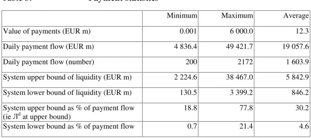
The data used in the simulations were collected from the Bank of Finland’s set-tlement account system. They cover all payments transferred in the Bank of Fin-land’s real-time gross settlement system (BoF-RTGS) between 4 January and 21 May 1999. The data cover the payments of 14 account holders and a dummy bank representing participants of the TARGET network. During the analysed period, the daily average number of payments was 1.790 and the average value was EUR 18.265 million. There are two peak times for payments in the system: one in the morning and one before the system closes. Between these peaks, the arrival rate of payments is rather stable, at 20-30 payments per minute. The settlement process starts each day at 8 am Finnish time and all payments entered into the system must be settled by the end of the day, at 7 pm. The characteristics of the data are summarized in table 3.

The large variations in number and settlement value of daily payments are due to the extended TARGET opening days. On national holidays, the domestic volumes are negligible and the volume of international transactions is also small. This also partly explains the variation in liquidity bounds. During the simulation period, the liquidity employed in BoF-RTGS averaged EUR 7.224 million and con-sisted of fully collateralized credit extended by the Bank of Finland worth EUR 5.664 million and compulsory reserve requirements worth EUR 1.560 million. The actual liquidity available to the participants was EUR 1.382 million more than the average upper bound, which indicates the existence of idle liquidity on some par-ticipants’ accounts. This resulted in quick settlements. The relatively large amount of liquidity used is due to the characteristics of the national settlement process. The very small number of participants combined with large differences in size and spe-cialization of system participants resulted in large fluctuations in payment flows. Some net settlement arrangements also ‘froze’ liquidity for the period for which the net settlement is calculated. The security settlement process in particular demands a large amount of liquidity for several hours during the day.

Table 3. 3D\PHQWVWDWLVWLFV

Minimum Maximum Average

Value of payments (EUR m) 0.001 6 000.0 12.3

Daily payment flow (EUR m) 4 836.4 49 421.7 19 057.6

Daily payment flow (number) 200 2172 1 603.9

System upper bound of liquidity (EUR m) 2 224.6 38 467.0 5 842.9

System lower bound of liquidity (EUR m) 130.5 3 399.2 846.2

System upper bound as % of payment flow

LH d

at upper bound)

18.8 77.8 30.2

System lower bound as % of payment flow 0.7 21.4 4.6

To some extent the Finnish figures are overstated, as some participants use the system as a liquidity source for euro outside Finnish markets and Finnish sectors of international markets.

The banks’ choice of payments to be settled at each moment depends inter alia on their available liquidity. In the data used, the choice of payments and the timing of settlement were recorded, as was the case for the actual settlement bal-ances and intraday credit limits. If an account holders’ liquidity changes, it is likely to settle its payments differently. The choice of settlement process is also likely to affect participants’ behaviour. However, for the purpose of this study we considered the payment data to be exogenously determined and not affected by the settlement structure or the liquidity available.

5

Simulations results

5.1

Relationship between liquidity usage and

settlement delay

The relationship between liquidity usage and settlement delay is analysed for re-gimes with rigid and flexible liquidity management systems. Figure 1 shows the relationship for a regime with rigid liquidity management for net and real-time gross settlement systems. A bank’s liquidity need in a multilateral net settlement system with end-of-day settlement is given by point A in the figure. In the simu-lations the system πG, ie participants’ total liquidity need as a share of total value of payments, was on average 5.1 %. If the number of net settlements during the day is increased, payment delay can be reduced in exchange for greater liquidity needs. Curve segment AC shows this tradeoff. If the number of settlements is in-creased to the point where net settlement is executed after each transaction (against earlier netted payments), the liquidity usage and settlement delay corre-spond to those of a real-time gross settlement system without queuing as well as to a CNS system with fully collateralized debt limits. This is shown as point C in figure 1, where πG equals 37.1 %.

Figure 1. 5HODWLRQVKLSEHWZHHQOLTXLGLW\XVDJHDQGVHWWOHPHQW GHOD\ULJLGOLTXLGLW\UHJLPH every 6h every 3 hours every hour 50% extra liquidity* 20% extra liquidity* lower bound C end-of-day B upper bound 0 % 20 % 40 % 60 % 80 % 100 % 0 % 5 % 10 % 15 % 20 % 25 % 30 % 35 % 40 %

Liquidity usage (_πd ) as % of total value of payments

1. Net settlement with different netting intervals

2. RTGS/CNS with queueing 1 2 A continuous S e tt lement delay , ρ

In an RTGS system with queuing facility, banks that are willing to accept more delay in their payments can reduce their liquidity usage by moving northwest on the tradeoff curve. This applies to CNS systems as well. The system level tradeoff curve, constructed by summing participants’ tradeoff curves, is shown as segment CB in figure 1. Liquidity must remain at least at the lower bound of liquidity (point B) if all payments during the day are to be settled. A bank can theoretically choose any point on its curve segment BC according to its preferences and esti-mate of relative costs of liquidity and delay. A bank that weights the cost of li-quidity high relative to that of settlement delay will choose a point near B and vice versa. The degree to which a system participant knows the shape of the curve before the end of the day will depend on its information as to incoming and out-going payments during the day. The range at which liquidity can be substituted for settlement delay is rather wide in our case, 32 % of the daily value of payments, on average. The curve is convex, with its slope being steeper than -1 up to the 70 % liquidity level and between -0.5 and -0.6 thereafter. Up to the 70 % liquidity level, an increase in liquidity usage is compensated by a larger relative reduction in settlement delay, after which the tradeoff becomes more gradual.

The curve representing different netting intervals in a net settlement system lies above the curve representing an RTGS system with queuing at all points be-tween the upper and lower bounds of liquidity. An RTGS (CNS) system can op-erate on the same amount of liquidity as any of the netting systems, with reduced payment (settlement) delay. In comparing end-of-day net and real-time gross set-tlement (both systems operating without counterparty risk), payment delay was found to be 62 % less for the RTGS system. Analogously, in comparing CNS systems, risks could be reduced by at least 62 %. The relative reduction in pay-ment or settlepay-ment delay was even larger in our comparison of an RTGS system operating on the same liquidity as netting systems with more frequent settlement intervals. At the six-hour interval the reduction amounted to 69 % and at the three- and one-hour intervals 84 %.

The relationship between liquidity usage and payment delay in a system with flexible liquidity management is very similar to that in the rigid regime. In the RTGS/CNS system, liquidity usage at the upper bound of liquidity was re-duced from 37.1 % to 27.5 % and at the lower bound from 5.1 % to 4.5 %. This is explained by the absence of idle liquidity in the flexible regime. The delays in payments are identical in both regimes. For net settlement systems the notion of flexible and rigid liquidity management was not considered relevant.

5.2

Combined cost of liquidity and delay

In figure 2 equal interest charges are applied to liquidity usage and to settlement (or payment) delay, and the total cost is plotted as a function of available liquidity. The reason for equal charges is that we would argue that the value of liquidity should be the same for the receiving and sending banks. An increase in the rela-tive price of liquidity bends the curves up on the right side and an increase in the relative cost of delay bends them up on the left side. If the relative price of liquid-ity (delayed payments) is high enough, the system-level cost-optimal liquidliquid-ity level is the lower (upper) bound of liquidity. An increase in either liquidity or delay costs will shift the curve up and a decrease will shift it down. An equal change in the cost elements does not affect the optimal allocation of liquidity.

combined cost is at its maximum with end-of-day net settlement, in which case all payments are delayed until the end of the day and liquidity usage equals the lower bound of liquidity. Reducing the interval of net settlements reduces the combined cost since the cost increase on liquidity usage is less than the cost reduction on settlement delay. The combined costs are thus minimized when net settlements are executed as often as possible, ie after each transaction, against previously settled payments.

The combined cost for an RTGS system with queuing in a rigid liquidity re-gime is shown as curve 2 in figure 2. At the lower bound of liquidity, delay costs are maximized and liquidity costs minimized. At the upper bound, costs stem solely from liquidity usage. System costs are minimized when the participants post liquidity worth 27 % of the total value of payments and liquidity is optimally allocated among participants. Below this level, dead-weight losses raise the com-bined costs; above it, the burden of increased idle liquidity reduces the costs.

Figure 2. &RPELQHGGDLO\FRVWRIOLTXLGLW\DQGVHWWOHPHQWGHOD\ ZLWKHTXDOLQWHUHVWFKDUJHVVKDUHRIGDLO\YDOXHRI SD\PHQWV end-of-day every 6h every 3h every hour continuous lower bound 3 0,000 % 0,001 % 0,002 % 0,003 % 0,004 % 0,005 % 0,006 % 0,007 % 0,008 % 0,009 % 0,010 % 0 % 5 % 10 % 15 % 20 % 25 % 30 % 35 % 40 %

Liquidity available as % of total value of payments

D a ily c o s t as % of t o ta l v a lue of pay ment s

1. Net settlement with different netting intervals 2. RTGS/CNS with queuing, rigid liquidity regime 3. RTGS/CNS with queuing, flexible liquidity regime

1

2

upper bound

The relative cost reduction in our case (with equal interest charges), as between real-time gross settlement and multilateral net settlement ranges from 59 % for end-of day net settlement to 20 % for netting at one-hour intervals. The only cost level at which the costs for net and gross settlement are equal is where payment delay does not entail any cost, ie where there is no need for intraday delivery. In this case end-of-day net settlement minimizes the costs for netting systems and the use of lower bound liquidity for real-time gross settlement systems.

The cost curves for RTGS systems operating under flexible and rigid li-quidity regimes are shown as curves 2 and 3 in the figure. The relative cost ad-vantage of the flexible liquidity regime compared to a rigid regime ranges from only 1 % at the lower bound of liquidity to 25 % at the upper bound. At the lower

bound the participants have very little idle liquidity on their settlement accounts; the amount of idle liquidity increases as more liquidity is made available. Intro-ducing flexibility when banks are operating at minimum liquidity has only a mi-nor impact on costs. It is presumably also the case that when banks operate with ample liquidity the reason is that they must have relatively low liquidity costs. Flexibility is a feature that can help banks overcome wider variations in liquidity demands at certain times of the day.

In systems where either payments or settlements can be delayed, partici-pants have the possibility to adapt to changes in relative costs of delay and liquid-ity. As the relative costs change, the cost curve shifts and a new optimal allocation of liquidity emerges. In net settlement systems based on end-of-day netting or pure RTGS systems without queuing, both liquidity need and settlement delay are determined solely by payment flows and hence the combined cost of settlement cannot be influenced by participants’ decisions. System-level cost-optimal liquid-ity usage for an RTGS system with queuing as a function of relative delay costs vs liquidity costs is shown in figure 3, for both flexible and rigid liquidity regimes. When the relative cost of settlement delay increases, banks find that reducing de-lay is more favourable and thus increase their liquidity holdings. In a flexible li-quidity regime when the cost of delay is equal to or less than 37 % of the cost of liquidity, the optimal allocation of liquidity is the lower bound. The cost of delay is small enough for participants to minimize their costs by simply posting just enough liquidity to enable settlement of all payments up to the end of the day. Between relative costs of 37 % and 75 %, participants will choose to delay a por-tion of their payments: the more, the less costly the payment delays relative to liquidity. If the cost of payment delays exceeds 76 % of the costs of liquidity, the optimum is to settle all payments immediately, in which case liquidity usage equals the upper bound.

Figure 3. /LTXLGLW\XVDJHLQDQ57*6V\VWHPZLWKTXHXLQJDV DIXQFWLRQRIUHODWLYHLQWHUHVWFRVWVRIGHOD\WROLTXLGLW\ 1 2 0 % 5 % 10 % 15 % 20 % 25 % 30 % 35 % 40 % 45 % 50 % 0 % 50 % 100 % 150 % 200 %

Relative interest cost of delay to liquidity

S ystem l iqui di ty usage,

1. RTGS/CNS with queuing, flexible liquidity regime 2. RTGS/CNS with queuing, rigid liquidity regime

lower bound upper bound

In a rigid liquidity regime, participants will operate at the lower bound of liquidity if the interest cost of delay is less then 52 % of the interest cost of liquidity. If the delay costs increase banks, will use more liquidity, which will reduce the delays. If delay costs are about twice as high as liquidity costs, the system-level cost-optimum is for each participant to post enough liquidity to settle its payments immediately. In a rigid liquidity regime, participants will tend to delay payments and thus incur higher delay costs because part of the delay cost is absorbed by the use of idle liquidity. In a flexible liquidity regime, the full costs are experienced by the receiver when payments are delayed and with more than 76 % of delay costs to liquidity costs, the system-level cost-optimum is not to delay payments.

5.3

Gridlocks in RTGS systems

Systems that operate with queuing face the risk of gridlock. In systems with cen-trally managed queues, the gridlocks are visible, whereas in systems with decen-tralized queue management they are normally hidden. We define gridlock as a situation where each participant of the settlement system is liquid, but not all payments can be settled immediately via the queuing algorithm due to the settle-ment order of paysettle-ments. In our model a participant is considered liquid during the analysed time period if its net liquidity position (the sum of incoming and outgo-ing queued payments combined with the available liquidity) is positive. If at least one of the system participants is illiquid, ie its net liquidity position is negative, the cause of any delays in settlement is not considered to be gridlock but rather insufficient funds. Our intention is to analyse how the system can be designed to prevent or solve gridlocks that occur despite the presence of sufficient liquidity.

The amount of gridlocks with the studied payment flows in an RTGS sys-tem with queuing is shown in table 4. Finnish banks operate at or above the upper bound of liquidity so that actual gridlocks were rare. As liquidity was reduced in the system, more gridlocks occurred, but even at the lowest levels of liquidity gridlocks were rather rare.

Table 4. *ULGORFNGXUDWLRQVDWGLIIHUHQWOHYHOVRIOLTXLGLW\LQ 57*6ZLWKTXHLQJ Lower bound (0 %) Low levels (10 %–30 %) Middle levels (40 %–60 %) High levels (70 %–90 %) Upper bound (100 %) Days experiencing gridlocks

(%) 28.0 7.3 5.3 5.0 0.0

Maximum time in gridlock

(tot. days, min) 35 35 70 73 0.0

Average time in gridlock

(of tot. days, min) 4.2 1.3 1.9 1.1 0.0

Average time in gridlock

(of days with gridlocks, min) 15.0 17.4 35.1 21.3 0.0

The average total duration of daily gridlocks was only 4.2 minutes at the lower bound of liquidity and 1.1 minutes at high levels of liquidity. On the worst day of the simulation period, with low levels of liquidity, the system was gridlocked for 73 minutes. With low levels of liquidity, the total duration of daily gridlocks was smaller but gridlocks occurred on more days, whereas at higher levels of liquidity

gridlocks occurred only on a few days but the duration was longer. Thus the over-all benefit of employing gridlock-solving algorithms is quite limited here.

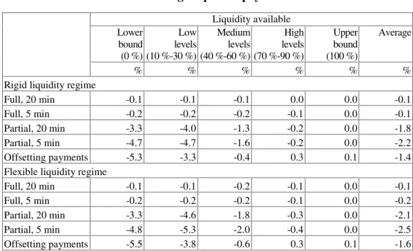
Gridlocks can be solved or prevented by using optimization methods like netting of queued payments or splitting large payments into several smaller ones. The effects of these optimization methods on gridlocks are summerized in table 5.

Table 5. &KDQJHVLQGDLO\JULGORFNGXUDWLRQZLWKGLIIHUHQW RSWLPL]DWLRQPHWKRGVLQ57*6V\VWHPV Liquidity available Lower Bound (0 %) Low levels (10 %-30 %) Middle levels (40 %-60 %) High levels (70 %-90 %) Upper bound (100 %) Upper bound (100 %) % % % % % %

Netting of queued payments

Full, every 20 min -41 -41 -73 -64 0 -57

Full, every 5 min -80 -83 -92 -84 0 -86

Partial, every 20 min -83 -94 -96 -88 0 -92

Partial, every 5 min -97 -98 -98 -91 0 -96

Offsetting payments -60 -75 -73 -100 0 -80 Splitting of payments Top 1‰ split 0 -3 0 0 0 -1 Top 1 % split -25 -82 -78 -55 0 -67 Top 5 % split -52 -100 -100 -98 0 -95 Top 10 % split -64 -100 -100 -98 0 -96

The netting of queued payments was simulated with full and partial netting and with 5- and 20-minute netting intervals. With full netting of queues every 20 minutes, the reduction in gridlocks amounted on average to 57 % and was maximized at medium and high levels of liquidity. If the netting was executed every 5 minutes, the reduc-tion averaged 86 % and the level of liquidity had less effect. The use of the partial netting algorithm reduced gridlocks still further. At the 20-minute netting interval, the average reduction was 92 % and at the 5-minute interval 96 %. Bilateral offset-ting of payments solved all gridlocks at the high levels of liquidity but was not as effective in reducing gridlocks when less liquidity was available to the participants. At the low and medium levels of liquidity, the reductions in daily duration of grid-locks were 60 % and 75 % respectively. Both full and partial netting substantially reduced the maximum daily time the system was gridlocked. The resulting total duration of gridlocks was reduced to approximately the time interval between the nettings. Only with bilateral offsetting of payments did the maximum total duration of daily gridlocks remain greater than a half hour at low levels of liquidity.

Splitting large payments into several smaller ones helps prevent the forma-tion of gridlocks. When the size of the payments is smaller, the amount of idle liquidity is less and a greater share of the available liquidity is employed for set-tlement. The effects of payment splitting on gridlocks are presented in table 5. Because only queued payments were split, the actual number of payments split varied according to the amount of liquidity available to the participants. At the lower bound of liquidity, the number of payments split was at its maximum, ie about half of the payments eligible for splitting. At the upper bound of liquidity,

of liquidity, but differences in efficiency were substantial. Splitting only the very large top 1‰ of payments (16 payments eligible for splitting during the 100-day period) had almost no effect on gridlocks, but splitting the top largest 1 % (1.733) already provided good results. Splitting the top 5 % (8.948) of payments was al-most as good as splitting the top 10 % (17.906) of payments even though the number of payments eligible for splitting more than doubled. With splitting of the top 5 % and top 10 % of payments, all gridlocks were eliminated at low and me-dium levels of liquidity, and at high of levels of liquidity the total duration of gridlocks was reduced by 98 %. This suggests that splitting of payments is techni-cally a very efficient method of alleviating the gridlock problem. Here, it was in many cases more effective than the netting algorithms, especially when over 5 % of transactions were split and when more than the lower bound of liquidity was available to the participants.

5.4

Optimizing an RTGS system

There are basically two ways to optimize settlement in real-time gross settlement systems: to clear gridlocks (and thus reduce delay costs) or to minimize the amount of idle liquidity. The latter applies to rigid liquidity regimes only because in flexible regimes banks can withdraw the idle liquidity from the system. For optimization methods such as payment splitting and netting queued payments, the curve representing the tradeoff between liquidity usage and settlement delay (fig-ure 1) can be shifted toward the origin and each participant can effect faster set-tlements with a given amount of liquidity.

The simultaneous settlement of several queued payments via netting clears gridlocks and thereby reduces settlement delay. However, in a real-time environ-ment there are some technical processing problems in applying netting algorithms, especially if these require prolonged calculation times. As payments are entered continuously into the system, the liquidity position of a participant might change as a result of payments settled while the net position is being calculated, if the system accepts new payments during the netting process. On the other hand, if the real-time process is suspended while netting is in process, there is a risk that pay-ments/settlements will be delayed. This requires rapid netting algorithms, espe-cially in systems with large volumes and many participants.

Table 6 summarizes the changes in the total cost of liquidity and delay with full or partial net settlement, 5- and 20-minute netting intervals, and bilateral offset-ting of payments. The results are calculated for both rigid and flexible liquidity re-gimes. The cost reduction was found to be similar for the two regimes, albeit the flexible regime resulted in a slight cost advantage. At the upper bound of liquidity, no queuing took place and the optimization methods had no effect. The effective-ness of full netting algorithms was very modest at all levels of liquidity: A reduction of only 0.1 % compared to non-netting was achieved at the 20-minute interval and a reduction of 0.2 % at the 5-minute interval. By using the partial netting algorithm for netting queued payments, costs were reduced substantially at low levels of li-quidity. The reduction was in the range of 4 % to 4.6 % for the non-netting scenario at the 20-minute interval and 4.7 % to 5.3 % at the 5-minute interval, depending on the liquidity regime. The bilateral netting of offsetting payments reduced the costs most at the lower bound of liquidity but was not as efficient as the partial netting algorithm at low and medium liquidity levels. At high levels of liquidity and at the upper bound of liquidity, the costs actually rose marginally. This can be ascribed to a change in the settlement order of payments that increased the liquidity needs.

Table 6. 5HODWLYHFKDQJHLQWRWDOFRVWVRIOLTXLGLW\DQGGHOD\ ZLWKQHWWLQJRITXHXHGSD\PHQWV Liquidity available Lower bound (0 %) Low levels (10 %-30 %) Medium levels (40 %-60 %) High levels (70 %-90 %) Upper bound (100 %) Average % % % % % %

Rigid liquidity regime

Full, 20 min -0.1 -0.1 -0.1 0.0 0.0 -0.1

Full, 5 min -0.2 -0.2 -0.2 -0.1 0.0 -0.1

Partial, 20 min -3.3 -4.0 -1.3 -0.2 0.0 -1.8

Partial, 5 min -4.7 -4.7 -1.6 -0.2 0.0 -2.2

Offsetting payments -5.3 -3.3 -0.4 0.3 0.1 -1.4

Flexible liquidity regime

Full, 20 min -0.1 -0.1 -0.2 -0.1 0.0 -0.1

Full, 5 min -0.2 -0.2 -0.2 -0.1 0.0 -0.2

Partial, 20 min -3.3 -4.6 -1.8 -0.3 0.0 -2.1

Partial, 5 min -4.8 -5.3 -2.0 -0.4 0.0 -2.5

Offsetting payments -5.5 -3.8 -0.6 0.3 0.1 -1.6

The splitting of payments prevents the formation of gridlocks and reduces the upper bound of liquidity, as the maximum liquidity constraint imposed by a pay-ment is reduced from its original value to the value of the splitting limit. Settle-ment delay is reduced as gridlocks are prevented but also because a part of the cover is available sooner to counterparties for settling their payments. Because, in the flexible regime, interest is calculated on the actual amount of liquidity em-ployed for settlement, the liquidity costs increase due to the fact that some of the liquidity is used sooner. The changes in total cost of liquidity and delay are sum-marized in table 7. Table 7. 5HODWLYHFKDQJHLQWRWDOFRVWVRIOLTXLGLW\DQGGHOD\ ZLWKSD\PHQWVSOLWWLQJFRPSDUHGWRDVFHQDULR ZLWKQRRSWLPL]DWLRQ Liquidity available Lower bound (0 %) Low levels (10 %-30 %) Medium levels (40 %-60 %) High levels (70 %-90 %) Upper bound (100 %) Average % % % % % %

Rigid liquidity regime

Top 0.1 % split -0.5 -0.7 -0.2 0.0 0.0 -0.3

Top 1 % split -4.6 -4.5 -1.6 -0.3 0.0 -2.1

Top 5 % split -9.3 -7.2 -2.7 -0.6 0.0 -3.7

Top 10 % split -10.7 -8.1 -3.1 -0.7 0.0 -4.2

Flexible liquidity regime

Top 1 ‰ split -0.5 -0.8 -0.1 0.0 0.0 -0.3

Top 1 % split -3.7 -0.5 3.2 1.6 0.0 0.8

Top 5 % split -6.6 1.2 5.6 2.9 0.0 2.0

In the rigid regime, costs are reduced more when a larger share of payments is split and when less liquidity is available to the participants. At the upper bound of liquidity all payments were settled immediately and no splitting was necessary. At high levels of liquidity the effects of all splitting limits were marginal, under 1 %. Also splitting the top 1‰ of payments had only minor effects on the costs. Split-ting the top 1 % of payments already provided notable results and a reduction in total cost of up to 4.6 % at the lower bound of liquidity, compared to a scenario without splitting.

From table 7 one can also see that in the flexible liquidity regime the total costs decline with payment splitting at low levels of liquidity but increase when more liquidity is available to the participants. Earlier use of liquidity increases the liquidity costs and, because the funds are available sooner to the receivers, the delay time and delay costs are reduced. At higher levels of liquidity the increase in liquidity costs is not fully compensated by the reduction in settlement delay costs and hence total costs are higher. With a flexible liquidity regime, a cost re-duction of 7.2 % could be achieved by splitting the top 10 % of payments, but a cost increase of 6.2 % occurred at medium levels of liquidity. When less pay-ments were split, both the reduction in costs at lower levels of liquidity and the increase in costs at medium and higher levels of liquidity were more modest.

Payment splitting entails some problems. Splitting can be achieved through an agreed upper limit for payment size (Humphrey 1996). It can also be imple-mented via an implicit and automated function within the settlement system and can be designed to be more or less transparent to the participants. For a system with payment splitting, the legal rules must take into account special situations in which payment processing is halted when only some parts of individual transac-tions have been processed.

6

Applicability of the findings and some

conclusions

The pattern of payment flows affects liquidity usage and the efficiency of the op-timization methods. The variations over time in payment flows can also lead to different results for different time periods. The characteristics of payment flows depend very much on market conventions and customer behaviour.

In addition to the simulations reported here, we have run simulations using Finnish payment data from other time periods and with artificially constructed payment flows. All of our key findings were supported by the results from these simulations. The absolute amounts of delay and liquidity usage varied but, in terms of efficiency, the rankings of different systems remained the same. Simula-tion is the best tool for determining exact properties of special types of settlement systems.

A further limitation is the exogenous character of payment flows. If the features of the settlement system were changed as drastically as in our models, it is likely that this would affect customer and system participant behaviour, which in turn would affect payment flows. We have not attempted to include these kinds of considerations in this study. Nonetheless, we feel that our approach is able to offer suggestions as to what kinds of enhancements to a given settlement system are worthy of deeper analysis.

The costs involved in payment systems are difficult to measure, especially delay costs, costs associated with settlement risk and, to an extent, liquidity costs. We have used simple linear cost functions, but in fact cost functions are probably highly nonlinear in some cases. However, even the rough cost estimates obtained here can be helpful in assessing the relative importance of different parameters. It is not a problem to include more realistic data in the model when these are avail-able.

Our main findings are as follows:

− A real-time system with queuing (ie RTGS/CNS or hybrid system) is always more efficient than a net settlement system with batch processing. For a given level of liquidity, the payment or settlement delay is always reduced by real-time processing, as compared to a time designated net settlement system.

− If liquidity costs are low enough relative to delay costs in an RTGS system, participants operate under immediate payment/settlement. Within a narrow range of relative costs of liquidity and delay, participants switch from maximum delay to immediate settlement. The central bank can support risk reduction and rapid payment targets by providing low cost intraday liquidity as well as more flexible ways for participants to add or withdraw liquidity from the system. Because the Finnish banking system is operating at or above the upper bound of liquidity, the current liquidity scheme adopted by the European System of Central Banks is providing efficient levels of li-quidity in terms of risk reduction.

− Optimizing and gridlock solving features are needed and effective only when liquidity is scarce. In the Finnish case, a splitting of the top 5–10 % of payments or partial netting of queues would be very efficient. The impact of different netting schemes is somewhat more limited. The available netting

− The costs of the settlement process can be reduced by applying optimization methods in situations with limited amounts of available liquidity. At very low levels of liquidity, these methods can be effective. The overall benefit depends of course also on the extra development and processing costs. The efficiency of the different optimization methods for settlement systems are affected by the actual flow of payments processed.

Our impression is that a simulation model similar to the one developed at the Bank of Finland is a useful tool for evaluating the properties of different settle-ment systems and processes s well as the impacts of changes in important system characteristics such as payment flows, settlement processes, cost and risk pa-rameters, and optimization methods.