Estimation of the Euro Area Output Gap Using the NAWM

(1)

WORKING PAPER SERIES

No 5 / 2009

ESTIMATION OF THE EURO AREA

OUTPUT GAP USING THE NAWM

(2)

WORKING PAPER SERIES

No 5 / 2009

ESTIMATION OF THE EURO AREA

OUTPUT GAP USING THE NAWM

1_{European Central Bank. The views expressed are those of the authors and do not} necessarily represent those of the European Central Bank.

2_{Bank of Lithuania. For correspondence: Economics Department, Bank of Lithuania,} Totorių g. 4, LT-01121 Vilnius, Lithuania; e-mail: [email protected]

(3)

© Lietuvos bankas, 2009

Reproduction for educational and non-commercial purposes is

permitted provided that the sourceis acknowledged.

Address

Totorių g. 4

LT-01121 Vilnius

Lithuania

Telephone +370 5 268 0132

Fax +370 5 212 4423

Internet

http://www.lb.lt

Statement of purpose

Working Papers describe research in progress by the author(s) and are

published to stimulate discussion and critical comments.

The Series is managed by Economic Research Division of Economics

Department

All Working Papers of the Series are refereed by internal and external

experts Disclaimer

The views expressed are those of the author(s) and do not necessarily

represent those of the Bank of Lithuania.

(4)

Estimation of the Euro Area Output Gap Using the NA WM / G. Co enen, F. Smets and I. V etlov

This paper presents preliminary estimates of the euro area flexible-price output gap using the estimated version of the New Area-Wide Model (NAWM) – a large-scale DSGE model of the euro area developed and maintained by ECB staff. Following a definition of the flexible-price output gap frequently used in the literature, we show that the NAWM-based measure may at times differ quite considerably from more traditional output gap measures and may display fluc-tuations of larger amplitude. The dynamics of flexible-price output is mainly driven by shocks to technology, whereas fluctuations in the output gap can be attributed equally to supply and demand shocks. We analyse how robust this output gap estimate is with respect to new incoming data and compare it’s inflation forecast performance with alternative measures.

Keywords: output gap, DSGE modelling, Bayesian inference, euro area.

JEL classification: C11, C32, E31, E32.

Santrauka

Pasitelkiant empirini˛ dinamini˛ stochastini˛ bendrosios pusiausvyros modeli˛ New Area-Wide Model (NAWM), šiame darbe pateikiami euro zonos gamybos atotr¯ u-kio esant lanksčioms kainoms i˛verčiai ir nagrin˙ejamos ju˛ savyb˙es. Taikant NAWM nustatyti 1998–2006 m. laikotarpio i˛verčiai reikšmingai skiriasi nuo i˛verčiu˛, gaunamu˛ taikant i˛prastini˛ gamybos atotr¯ukio skaičiavimo b¯udą, jie pasižymi didesniais svyravimais. Gamybos lygio kitimas esant lanksčioms kai-noms labiausiai priklauso nuo technologin˙es pažangos šoku˛, o gamybos atotr¯ukiui i˛takos turi tiek pasi¯ulos, tiek paklausos šokai. Nustatyti gamybos atotr¯ukio rekursiniai i˛verčiai yra gana pastov¯us, o tai rodo ju˛ dideli˛ patikimumą skai-čiuojant gamybos atotr¯uki˛ realiuoju laiku. Palyginus pateikiamus i˛verčius su i˛prastiniais gamybos atotr¯ukio vertinimais, matyti, kad šiame darbe pateikia-mas gamybos atotr¯ukio skaičiavimas teikia daugiau vidutinio laikotarpio in-fliacijos prognozavimo galimybiu˛.

(6)

1 Introduction

An increasing number of central banks, including the European Central Bank (ECB), are using calibrated or estimated New Keynesian Dynamic Stochastic General Equi-librium (DSGE) models as useful tools for monetary policy analysis and economic projections.1 _{These models typically combine a neo-classical Real Business Cycle}

model with sticky nominal prices and wages that can lead to inefficient business cy-cle fluctuations in response to various economic shocks. Endowed with a sufficient number of structural shocks, they also provide a relatively good empirical fit.2 _As

argued by Woodford (2003) and, more recently Galí and Gertler (2007), in the New Keynesian framework natural (i.e. flexible-price equilibrium) values of both output and the real interest rate can provide important reference points for monetary pol-icy for two reasons. First, those natural rates may reflect the constrained efficient level of economic activity and therefore may feature in the objective functions of welfare maximising central banks. Second, monetary policy cannot create persistent departures from those natural levels without inducing either inflationary or defla-tionary pressures. In spite of the increasing use of New Keynesian DSGE models in policy institutions, there has been relatively little analysis of the properties of the flexible-price output and interest rate levels in estimated models. One reason may be that those estimates are quite a bit different from more traditional estimates of potential output or the equilibrium real interest rate, which typically are modelled as smoothed trends.3

In this paper we analyse a notion of flexible-price output and output gap based on the estimated New Area-Wide Model (NAWM) developed at the ECB.4 _{The output}

gap notion used in the monetary policy reaction function of the current specification of the estimated NAWM is closely related to traditional measures of the output gap. It is defined in terms of the deviation of actual output from trend output, which captures the permanent component of the actual output series. In documenting properties of this output gap measure, Coenen and Vetlov (2008) find that this measure is highly correlated with measures of the euro area output gap derived from more traditional macroeconometric and unobserved component models. However, the NAWM-based measure displays business-cycle fluctuations of considerably larger amplitude. In this paper, we confront this more traditional measure with a version of a flexible-price output gap. More specifically, in line with the related DSGE

1_{Early examples of New Keynesian DSGE policy models are Ramses at the Sveriges Riksbank}

(see Adolfson, Laseén, Lindé, and Villani (2007) for details) and ToTEM at the Bank of Canada (see Murchison and Rennison (2006) for a detailed description).

2_{See, for example, Smets and Wouters (2005) for a more elaborate description of the advantages}

of Bayesian New Keynesian DSGE models.

3_{See, for example, Smets and Wouters (2003), Edge, Kiley, and Laforte (2007) and Justiniano}

and Primiceri (2008).

(7)

Bank of Lithuania W orking P ap er Series No 5 / 2009

literature, the baseline flexible-price output gap is defined as the deviation of actual output from the counterfactual level of output that would prevail in an environment of full nominal flexibility in goods and labour markets and absent shocks to price and wage markups (Woodford (2003)). This notion was also used in Smets and Wouters (2003), Edge, Kiley, and Laforte (2007) and, very recently, in Justiniano and Primiceri (2008). As argued by Neiss and Nelson (2005), this concept of the output gap implied by DSGE models is not a measure of the business cycle. Instead, its primary role is to inform policymakers about disequilibria in goods and labor markets that are implied by the presence of nominal rigidities.5

Conceptual differences in defining potential output and output gaps have im-portant implications for the time-series properties of output gap estimates implied by different approaches. Compared to the traditional approaches, which implic-itly assume that potential output is driven by permanent technology shocks, the DSGE approach assumes that other shocks, for example temporary productivity shocks, various demand shocks and terms-of-trade shocks, can also affect potential (i.e. flexible-price) output dynamics over the business cycle. As a result, applications of the DSGE approach may produce more volatile estimates of potential output, and smaller and less persistent estimates of the output gap, when compared to the cor-responding estimates obtained using the traditional approaches. Whether this is the case will, however, depend on the specification of the model and the stochastic pro-cesses governing the structural shocks. For example, Justiniano and Primiceri (2008) argue that the flexible-price output gap they derive for the US is quite similar to more traditional measures of the output gap, as long as the effects of price and wage mark-up shocks on the flexible-price level of output are excluded.

As discussed above, despite theoretical appeal and impressive advancements in building empirical DSGE models, active use of flexible-price output gap in policy-making institutions remains limited. To some extent this seems to reflect the fact that the operational definition of flexible-price output gap has not been settled yet by the profession. There are remaining issues regarding the robustness of the flexible-price gap estimates with respect to alternative model structures, shock identification schemes, data revisions, etc. Moreover, when compared to the traditional methods, the DSGE approach to output gap estimation is more involved technically and, in some cases, may appear less transparent for non-modelers. Arguably, there is large scope for more empirical work on flexible-price output gaps as relevant existing litera-ture remains scarce. The contribution of this paper, therefore, is to further illustrate the empirical properties of the flexible-price output gap in a particular estimated DSGE model that is designed to be used in a policy environment. In addition, we investigate how robust this estimate is with respect to new incoming data and analyse how useful these measures are in predicting inflation.

(8)

In the remainder of the paper, we first summarize the structure of the estimated NAWM. Section 3 then presents estimates of the flexible-price level of output and the associated output gap based on the NAWM. In this section, we examine the various sources of fluctuations in the output gap and investigate the robustness with respect to real time estimation and the inclusion of alternative sets of shocks. In Section 4, we then investigate the usefulness of our baseline estimate of the flexible-price output gap for gauging inflationary pressures in the euro area. This is based on a forecast comparison exercise for inflation at various horizons. Finally, the paper concludes by summarizing the key findings and by discussing remaining open issues.

2 The NAWM: Specification and Estimation Issues

In this section we give a quick overview of some of the important features of the NAWM.6 _{The NAWM is a micro-founded open-economy model of the euro area}

under development at the ECB, which is primarily designed for use in the (Broad) Macroeconomic Projection Exercises regularly undertaken by ECB/Eurosystem staff. The model in its log-linearized form is estimated with Bayesian techniques using 18 macroeconomic variables over the sample period ranging from 1985q1 to 2006q4 (utilizing the period 1980q2 to 1984q4 as training sample).

Regarding the NAWM structure, there are four types of economic agents in the domestic (euro area) economy: households, firms, a fiscal authority and a mone-tary authority. Households make optimal choices of consumption and investment in physical capital; they supply differentiated labour services, set wages, and trade in domestic and foreign bonds. Regarding firms, there is a distinction between domestic monopolistically competitive producers of tradable differentiated intermediate goods and competitive producers of three non-tradable final goods: a private consumption good, a private investment good, and a public consumption good. Intermediate-good firms use labour and capital as inputs to produce their differentiated good, which they sell both domestically and abroad. They also set the prices of those goods. In addition, there are foreign intermediate-good producers that sell their differentiated goods in domestic markets, and a foreign retail firm that combines the exported do-mestic intermediate goods for final consumption abroad. Final-good firms combine domestic and foreign intermediate goods into private and public consumption goods and private investment goods. The fiscal authority purchases public consumption goods, issues bonds, and levies different types of taxes.7 _{The monetary authority}

sets the nominal interest rate by following a Taylor-type interest-rate rule. Interna-tional linkages arise from the trade of intermediate goods and internaInterna-tional assets, allowing for limited exchange-rate pass-through and imperfect risk sharing.

6_{Full documentation of the model’s estimation procedure and properties is provided by}

Christof-fel, Coenen, and Warne (2008).

(9)

Households and firms face nominal and real frictions, which render re-adjustments of intertemporal decisions costly and give rise to plausible adjustment dynamics. Real frictions are introduced via external habit formation in consumption, gen-eralised adjustment costs in investment and in the import content of final goods, fixed costs in intermediate-good production and through monopolistic competition in intermediate-goods and labour markets. Nominal frictions arise from assuming sticky prices and wages á la Calvo and (partial) dynamic indexation. In addition, there are financial frictions in the form of an exogenous "external finance premium" and intermediation costs for trading foreign bonds.

While the euro area economy in the NAWM is characterized by a detailed micro-founded structure, the rest-of-the-world block is represented by a structural vector-autoregressive (SVAR) model explaining the dynamics of foreign variables: demand, output prices, interest rate, competitors’ export price and oil price. The SVAR is estimated separately from the core NAWM and features no spill-overs from the euro area block to the rest of the world.

The NAWM incorporates numerous stochastic processes: 12 structural shocks (permanent technology, transitory technology, investment-specific technology, do-mestic risk premium, import demand, export preference, interest rate, external risk premium, wage markup, price markup of domestic goods sold domestically, price markup of domestic goods sold abroad, and price markup of foreign goods sold do-mestically), 5 shocks in the SVAR model capturing the rest of the world (foreign de-mand, foreign interest rate, foreign price, competitors’ export price, oil price shocks) and 1 shock in a univariate autoregressive (AR) model for government consumption (government consumption shock). All shocks are assumed to follow first-order au-toregressive processes, except for the interest rate shock and the shocks in the AR and SVAR models, which are assumed to be serially uncorrelated.8

The model features two unit root processes. The first one underlies the evolu-tion of labour-productivity growth. In line with the balanced-growth property of the model, all real variables, with the exception of hours worked, share a common real stochastic trend. The second unit root process arises due to the fact that the monetary authorities aims at stabilising inflation relative to its objective, rather than the price level, thus, all nominal variables share a common nominal stochastic trend. In this regard, in order to render the model stationary, when estimating the model, all variables that contain a real trend are scaled with the level of productivity zt, while all variables that contain a nominal trend are scaled with the price of the con-sumption good. Furthermore, to account for demographic trend in the data, all real

8_{In addition, measurement error is introduced in extra-euro area trade data (both volumes and}

prices) in view of the fact that they are prone to large revisions. Small errors in the measurement of real GDP and the GDP deflator are allowed for to alleviate differences between the national accounts framework underlying the construction of official GDP data and the NAWM’s aggregate resource constraint.

(10)

variables, are also scaled by an assumed deterministic trend in labour force. The latter is calibrated to grow at 0.2 per cent each quarter.

Focusing on the level of productivity, more formally, z_t is defined as a random walk with drift:

zt = gz,tzt−1, (1) gz,t = ρgzgz+ (1−ρgz)gz,t−1+η

gz

t , (2)

wheregz,trepresents the (gross) rate of labour-augmenting productivity growth with steady-state valueg_z,ρ_g_z measures the degree of persistence of changes in trend pro-ductivity growth, and ηgz

t denotes i.i.d. innovations to trend productivity growth. The deterministic part of the labour productivity process,gz, is fixed at 0.3 per cent per quarter which approximates the average quarterly growth rate of labour produc-tivity observed over 1990–2006. The stochastic part of the producproduc-tivity process,ηgz

t , is identified from the smoothed estimates of the state shocks using the Kalman filter when inverting the model on a given set of observed variables.

As a result, the real steady state level of the NAWM is given by essentially a stochastic trend comprising a drift component given by deterministic trends in the labor force and labor productivity (implying 2 per cent deterministic growth in output on annual basis) and a stochastic component represented by a sequence of shocks to technology (labor-augmenting technological progress). For the rest of the paper, unless otherwise indicated, the NAWM-based real variables will be reported in percentage deviation from the stochastic trend just defined.

3 Output Gap Estimates Based on the NAWM

In this section, we analyse the characteristics of the flexible-price output gap derived from the NAWM over the European Monetary Union (EMU) period. Following a section on the definition of the flexible-price output gap, we analyse the properties of the flexible-price output level, the associated output gap and its robustness with respect to real-time estimation and the inclusion of various shocks.

3.1 Definition of Flexible-Price Output (Gap)

As in Smets and Wouters (2003), Edge, Kiley, and Laforte (2007) and Justiniano and Primiceri (2008), we define the baseline flexible-price output gap as the deviation of actual output from the counterfactual level of output that would prevail in an environment of full nominal flexibility in goods and labour markets and absent shocks to price and wage markups. In terms of practical modeling, a flexible-price block has been added to the original model as a parallel economy in which price and wage

(11)

setting is fully flexible and there are no shocks to wage and price markups. All other (or efficient) shocks identified in the original model are allowed to affect output in the flexible-price block. Compared to the original model structure, there is no monetary policy rule in the flexible-price block. The real interest rate is obtained implicitly via the consumption Euler equation, while the growth rate of the numeraire price (the price of the consumption good) is set to zero.

More formally, assuming full nominal flexibility, the wage curve in the flexible-price block is reduced to the following expression:

ˆ wt = µ 1 1−¯τN₋_τ_¯W h ¶ (ˆτ_tN + ˆτ_tW h) +mrsdt, (3) where wˆt is gross real labor compensation, τˆtN and τˆtW h denote the labor income tax rate and social security tax rate respectively paid by households, and mrsdt is marginal rate of substitution between consumption and leisure. A hat on top of the variable denotes that the variable is expressed in terms of the logarithmic deviation from its steady state value.

Prices of domestic intermediate goods sold domestically and abroad as well as prices of foreign goods sold domestically are set equal to nominal marginal cost of respected production so that real marginal cost measures do not deviate from their steady state value:

ˆ

pt = mcct, (4)

wherepˆ_t is the relative price, andmcc_t is nominal marginal cost of production. Three issues are worth mentioning in relation to this definition of the flexible-price output gap. First, although the flexible-flexible-price economy is run in parallel to the actual sticky-price economy, the state or predetermined variables of the flexible-price economy are set to their actual realisations in the sticky-flexible-price economy. In the NAWM, those state variables do not only include the capital stock, but also many lagged variables such lagged consumption, investment, wages and inflation. This assumption is similar to more traditional production function approaches where the capital stock is often assumed to be given by its historical value. Our definition is similar to what Woodford (2003) defines the natural rate of output and Adolf-son, Laseén, Lindé, and Svensson (2008) call the conditional output gap. AdolfAdolf-son, Laseén, Lindé, and Svensson (2008) distinguish the conditional output gap, which takes the pre-determined variables as given and assumes that prices and wages sud-denly become flexible in the current period and are expected to remain flexible in the future, from the unconditional output gap, which assumes that the economy has always featured flexible wages and prices but was subject to the same shocks as the actual economy. The latter definition resembles the notion of natural rate of output

(12)

consistent with the natural interest rate provided by Neiss and Nelson (2003). Adolf-son, Laseén, Lindé, and Svensson (2008) study how the use of these different notions of the output gap in a central bank loss function affect optimal policy projections.9

Second, following Smets and Wouters (2003) it has become common to exclude the stationary exogenous stochastic component of wage and price mark-ups from the definition of the flexible-price level of output. Justiniano and Primiceri (2008) call this potential output, as opposed to natural output in which also wage and price mark-up shocks affect the flexible-price output level. In line with the analysis in Woodford (2003), Smets and Wouters (2003) argue that from a monetary policy point of view the notion excluding mark-up shocks is more appropriate because these shocks give rise to inefficient variations in the flexible-price level of output and thus monetary authorities should not try to accommodate such variations. Of course, in this case mark-up shocks will give rise to a potential trade-off between inflation stabilisation and output gap stabilisation. In the context of a model that is very similar to that in Smets and Wouters (2007), Justiniano and Primiceri (2008) make a somewhat different argument in favour of excluding the price and wage mark-up shocks. They argue that the price and wage mark-mark-up shocks are not very well micro-founded and show that a model with measurement error in the price and wage equations without mark-up shocks does a somewhat better job in fitting the data.10

Finally, a third issue of estimating the flexible price output gap using the NAWM arises due to the open-economy nature of the model. As the rest of the world is modelled through a reduced-form model, it is not possible to distinguish efficient from inefficient variations in foreign variables (with the exception of price setting on foreign goods sold in the euro area for which a structural relationship is explicitly defined). In the baseline definition of the flexible-price output gap, we treat all foreign variables as exogenous and let them affect the flexible-price output level in the euro area.

3.2 Trend and Flexible-Price Output Level

In this section, we first look at estimates of the flexible-price output level itself. Figure 1 displays the NAWM-based estimates of the euro area flexible-price and trend output level as well as actual real GDP over the EMU sample of 1999q1–2006q4. As discussed in above, trend output refers to the stochastic balanced-growth path of the model comprising a drift component given by deterministic trends in the labor force and labor productivity and a stochastic component represented by a sequence of permanent technology shocks.

9_{From a loss function perspective, the unconditional output gap may be more appropriate than}

the conditional output gap because the latter lets bygones be bygones, i.e. policy mistakes that have led to deviations of predetermined variables from their efficient levels are accommodated.

10_{A similar criticism of the wage mark-up shocks can be found in Chari, Kehoe, and McGrattan}

(13)

Figure 1 shows that estimated trend output displays a high degree of smooth-ness, similar to traditional estimates of potential output based on univariate linear de-trending techniques. This can be explained by the fact that the NAWM-based estimates of the permanent technology shocks are relatively small in size and display a substantial degree of persistence.

Figure 1: Estimates of flexible-price output in the NAWM (on a logarithmic scale)

Figure 2: Decomposition of flexible-price output in the NAWM (in per cents)

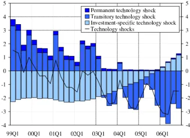
In contrast, the estimated flexible-price output level features distinct short-run fluctuations, but similar to the stochastic trend it does not reveal much of a cyclical pattern. Most strikingly, the flexible-price output level displays a distinct downward shift relative to trend output over the EMU period. The sources of this downward shift can be further investigated by inspecting the contributions of the NAWM-based structural shocks to the deviation between trend and flexible-price output, as displayed in Figure 2. For expositional clarity, the shocks are grouped into two cate-gories: technology shocks (permanent, transitory and investment-specific technology

(14)

shocks) and other shocks (essentially demand and foreign shocks). As expected, the slowdown in flexible-price output is mostly due to the overall negative impact of technology shocks.

A further breakdown of the technology shocks shown in Figure 3 reveals that most of the gradual slowdown over this period is due to a series of transitory, but persistent, technology shocks. In the first half of the sample, positive shocks were largely offset by negative investment-specific technology shocks. In the later part of the sample, a series of negative temporary technology shocks is the main source of the slowdown (see Figure 4). These negative shocks are associated with a strong pick-up in investment and employment since 2003, which was not equally matched by a recovery in domestic consumption.

Figure 3: Decomposition of technology shocks’ contribution to flexible-price output in the NAWM (in per cents)

Figure 4: Smooth estimates of the transitory technology shock and flexible-price output in the NAWM (in per cents)

(15)

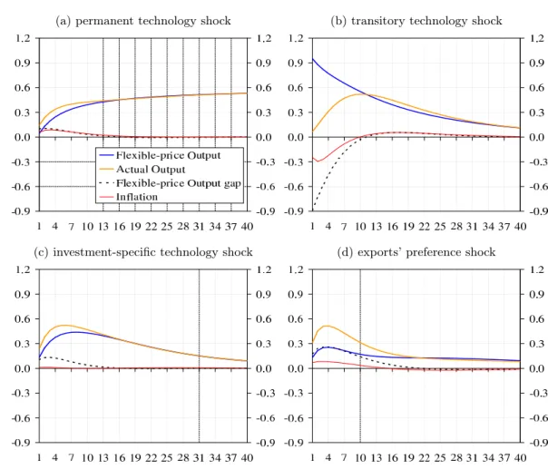
In order to better understand the impact of the various shocks on the flexible-price output level, Figures Ia-Ic and Figure Id in the Annex show the response of actual and flexible-price output to respectively three technology shocks and one typi-cal demand-side shock (an export-preference shock). In all cases the size of a shock is given by one standard deviation. Several observations are worth mentioning. First, differences in the responses of actual and flexible-price output are short-run phe-nomena that gradually vanish over the longer horizon. Second, within the group of technology shocks, the largest difference in response is found in the case of a transi-tory technology shock. This shock has a considerably quicker and larger impact on the flexible-price output as compared to actual output for which the impact is signif-icantly reduced and delayed by the presence of nominal rigidities. Nominal rigidities appear to limit the spill-over of the volatility in the marginal costs of production, induced by the shock, on the rest of the economy, thus, facilitating smoother overall macroeconomic dynamics. Third, demand-side shocks, as exemplified by response to an export preference shock, have clearly smaller and a less persistent impact on flexible-price output compared to their impact on actual output. This also explains why, as expected, demand-type shocks play only a limited role in driving estimates of the flexible-price output level.

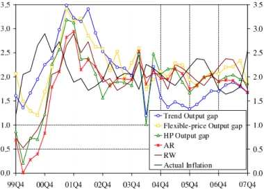
3.3 Flexible-Price Output Gap

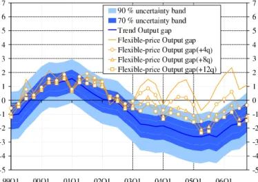
Next, we analyse the NAWM-based estimate of the flexible-price output gap. Figure 5 displays this estimate as well as the NAWM-based trend output gap and a more traditional output gap derived by applying the Hodrick-Prescott (HP) filter with a smoothness parameter set to 1600. In addition, we report the 90 and 70 percent confidence set of the estimated flexible-price output gap.

Figure 5: Estimates of flexible-price output gap in the NAWM (in per cents)

(16)

flexible-Estimation of the Euro Area Output Gap Using the NA WM / G. Co enen, F. Smets and I. V etlov

price output gap features a relatively high degree of volatility, mostly reflecting the higher volatility of the flexible-price output level discussed in the previous section. Interestingly, while all measures have a similar hump-shaped profile and appear to be highly correlated in the earlier period (1999–2002), since 2003 the wedge between the alternative output gap estimates increased. Moreover, due to the downward shift in the flexible-price output level in the latter period, the flexible-price output gap level is mostly positive since 2002, whereas the more traditional output gaps indicate a negative gap.

This different behaviour can be better understood by analysing the historical de-composition of the flexible-price output gap level with respect to the various struc-tural shocks, as displayed in Figure 6 (see also the corresponding decomposition of four-quarter change in the output gap in Figure II in the Annex). For expositional clarity, the shocks are grouped into five categories: technology, demand, markups, monetary policy, and foreign shocks.11

Figure 6: Decomposition of flexible-price output gap in the NAWM (in per cents)

In the first half of the EMU period, the output gap is mostly driven by demand and foreign shocks associated with the bursting of the dot-com bubble and the early millenium slowdown, which may explain why all three measures give similar indi-cations. Since 2003, the euro area seems to have been hit by negative productivity developments, which push down the estimated flexible-price output level and drive

11_{The technology shocks include permanent technology shock, transitory technology shock, and}

investment specific technology shock. The demand shock category includes domestic risk premium shock, import demand shock, and innovation to government consumption. The markup shocks include wage markup shock, domestically sold home goods price markup shock, and exports price markup shock. The monetary shock is given by an interest rate shock. The foreign shocks include external risk premium shock, innovation to foreign demand, innovation to foreign inflation, innova-tion to foreign interest rate, export preference shock, imports price markup shock, and innovainnova-tion to competitors’ prices. Possible discrepancies between the sum of the contributions and the esti-mate of the output/growth gap in a given quarter may arise due to impact of the initial state, the contribution of which is not reported in the charts for presentational purposes.

(17)

an increasing wedge between the flexible-price output gap and the more traditional measures of the output gap. According to the estimates of the NAWM, the negative contribution of demand shocks following the economic growth slowdown in 2002–2004 are mostly offset by positive contributions from monetary policy. The net effect is an estimated positive output gap through most of the latter period.

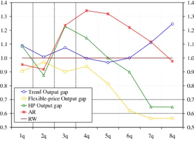
Figure 7: Convergence of the medium-term notion of the flexible-price output gap towards the trend output gap level (in per cents)

Note: The uncertainty bands refer to estimates of the trend output gap. The medium-term notion of the flexible output gap obtained by considering 4, 8, and 12 quarter ahead model-based forecast of the flexible-price output level.

As discussed in the previous section, the downward shift of flexible-price output relative to trend is mostly due to the immediate, but temporary effects of temporary productivity shocks on flexible-price output. The impact of those shocks fades away over time. One way of reducing the difference between the flexible-price and the trend output gap is therefore to use forecasts of the flexible-price level of output as potential output. This will tend to make estimates of the flexible-price output level smoother. Moreover, as the forecast horizon lengthens, the corresponding flexible-price output gap will converge to the trend output gap. Indeed, Figure 7 shows that the medium-term notion of the flexible-price output gap gravitates towards the trend output gap as forecast horizon increases. In fact, except for a very few quarters, the flexible-price output gap computed on the basis of 8 quarter ahead forecast of the flexible-price output is not significantly different from the trend output gap.

3.4 Robustness

How robust are the estimates of the flexible-price output gap? As discussed above, domestic demand or foreign shocks have only limited impact on the flexible-price level of output. As a result, excluding those shocks from affecting the flexible-price output level does not have much of an effect on the properties of the resulting

(18)

output gap. What turns out to be of much greater importance is whether one allows markup shocks to affect the flexible-price output level. In this case, two changes become apparent. First, the volatility of the estimated output gap increases a lot. A similar, but more extreme, finding has been reported by Justiniano and Primiceri (2008) when deriving natural output estimates in a version of the Smets and Wouters (2007) model for the United States. Differently from their finding, we find that the output gap estimates are sensitive to the inclusion of not only wage mark-up shocks, but also price mark-up shocks. The primary explanation behind this high sensitivity of the volatility of the estimated output gap to the inclusion of mark-up shocks is the high estimated volatility of those shocks. Justiniano and Primiceri (2008) argue that a part of the so-called mark-up shocks may capture measurement error in prices and wages.

Second, in the euro area also the level of the output gap is affected. Since the mid-1990s, the wage mark-up shocks have systematically been negative reflecting a falling labour share and a period of wage moderation (see Figure 8). This tends to push up the flexible price output level and reduce the associated output gap. In contrast, the price mark-up shocks have shown a upward trend in the EMU period, partly reflecting cost-push shocks due to higher energy and commodity prices that are not explicitly modelled. This tends to lower the flexible-price output.

Figure 8: Smooth estimates of the wage and domestic price mark-up shocks in the NAWM model (in per cents)

As argued by Justiniano and Primiceri (2008) and Chari, Kehoe, and McGrat-tan (2008), the structural interpretation of the so-called mark-up shocks can be questioned. For example, the wage mark-up shocks are observationally equivalent to labour supply shocks, with very different welfare implications (see Smets and Wouters (2003)). Only with more data and a better modelling of the labour market can we hope to clearly distinguish between those different forces. Similarly, as argued

(19)

Bank of Lithuania W orking P ap er Series No 5 /

2009 by de Walque, Smets, and Wouters (2006), price mark-up shocks are observationally_{equivalent to relative price shocks in a flexible-price good sector. Again, with very} implications for the calculation of the flexible-price output as a consequence. Dis-entangling these different sources of the historical movements in the mark-ups is an important area for future research, which will affect the calculation of the appropriate flexible-price output gap.

Figure 5 above shows that the estimated shock and parameter uncertainty around the flexible-price output gap isn’t that large. Typically the 90% confidence set is about 1 percentage point wide. An additional issue worth investigating is how robust the flexible-price output gap estimates are with respect to data revisions and model re-estimation.

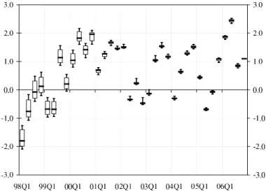
Figure 9 reports the summary statistics of a pseudo real-time estimation of the flexible-price output gap, starting with the initial sample spanning the period 1985q1–1998q4 and re-estimating the gap with each additional quarter. In this ex-ercise, the model parameters are re-estimated only every fourth quarter. For each quarter we show the minimum and maximum (thin black vertical bar), median (black horizontal line) and interquartile (denoted by a box) of the output gap estimates. Summary statistics of the recursive estimates of the NAWM-based trend as well as the HP output gaps are displayed in Figures IV and V in the Annex.

Figure 9: Revisions to the NAWM-based flexible-price output gap estimates (in per cents)

The figure reveals rather moderate revisions in the level of the output gap as new data comes in. Compared to recursive estimates of the NAWM-based trend output gap, size of revisions to the flexible-price output gap shrinks rapidly towards the end of the sample. This exercise contrasts the findings with more traditional measures of the output gap that there is substantial uncertainty in estimates of the level of the

(20)

output gap due to incoming data.12

In this paper, we take the structure of the NAWM as given. Additional un-certainty surrounding the output gap measures may be due to unun-certainty about the specification of the NAWM including its structural shocks. Future research will need to assess to what extent estimates of the flexible-price output gap are robust to changes in the specification of the NAWM.

4 Output Gaps as Predictors of Inflation

As argued in the introduction, within the New Keynesian framework flexible-price output gaps should be good indicators of inflationary or deflationary pressures. In this section we explore the predictive content of the NAWM-based flexible-price out-put gap for euro area inflation at various horizons. Since the seminal work of Phillips (1958) reduced-form relationships between real activity and prices have frequently been exploited by modelers for forecasting future inflation. While forecast accu-racy of early versions of the Phillips curve largely deteriorated in the seventies, the search for a proper specification of Phillips curves continues as output and/or unem-ployment gaps remain some of the key indicators considered by many policymaking institutions. Stock and Watson (2008) review the recent literature on pseudo out-of-sample evaluation of Phillips curve-based inflation forecast models in the United States. An important benchmark in this regard is Atkeson and Ohanian (2001), which analyzes US GDP deflator growth over period 1984–1999 and shows that, in terms of forecast accuracy, naïve benchmarks, such as smooth random walk, can easily outperform Phillips curve-based models that rely on output gaps or other measures of economic slack. Stock and Watson (2008) show that relative forecast performance of the Phillips curve may be episodic. In periods of a stable macroe-conomic environment the Phillips curve-based forecasts are outperformed by naïve models, whereas in the face of large business cycle swings forecast accuracy of the former improves considerably over the latter.

In this section, we explore the value of the NAWM-based output gaps for fore-casting inflation in the private consumption deflator in the euro area.

4.1 Forecast Evaluation Procedure

Our forecast evaluation procedure is based on an approach similar to the one applied by Fischer, Lenza, Pill, and Reichlin (2006) in studying the performance of money-based inflation forecasts in the euro area. In particular, the pseudo out-of-sample forecast of inflation is obtained on the basis of bivariate models which are estimated on rolling samples of 40 quarters in pseudo-real time, with 33 vintages of quarterly data (with the initial sample spanning 1985q1–1998q4 and the final sample covering

(21)

Bank of Lithuania W orking P ap er Series No 5 / 2009 1985q1–2006q4).

13 _{The mean squared forecast errors (MSFE) of the output gap}

models are then compared to the MSFE of benchmark models, which in our case are limited to a smooth random walk and univariate autoregressive models of inflation. More formally, we consider forecasting the annualizedh-period change in private consumption deflatorπh t+h: πh_t₊_h = 100∗ Ãµ Pt+h P_t ¶4 h −1 ! , (5)

wherePt is price level att,h is forecast horizon in quarters.

The general specification of the bivariate models for each vintage of datav is as follows: πh_v,t₊_h = av+bv(L)πv,t+cv(L)xv,t+²h,x_v,t₊_h, (6) where πv,t = 400∗ ³ Pt Pt−1 −1 ´

is the annualized one-period change in private con-sumption deflator,xv,t is output gap,bv(L)andcv(L)are finite polynomial of order

pand q.

The forecasting models are estimated by Ordinary Least Squares (OLS). Starting with general specification of four lags for both inflation and output gap, lags for dependent variables are then selected using the Schwartz information criteria.

For each data vintage, based on the final specification in (6) a forecast of inflation is obtained:

πh,x_v,t₊_h =aOLS_v +bv(L)OLSπv,t+cv(L)OLSxv,t.

The autoregressive models of inflation are estimated following the same procedure described above. The random walk forecast of inflationh period ahead is given by Atkeson and Ohanian (2001) random walk model where inflation forecast is given by the average rate of inflation over the previous four quarters available for a given data vintage14_: π_v,th,RW₊_h = 100∗ µ P_t Pt−4 −1 ¶ . (7)

Forecast errors et for the generic forecast from modelMare defined as:

eh,_t₊M_h = π_v,th,M₊_h−πh_t₊_h, (8) whereπh

t+h is the realized inflation rate in the last available vintage of data.

13_{We chose rolling sample estimates to put the rival forecasting models on a more equal footing,}

since under recursive estimation method the RW may have advantage over alternative models by using the most recent inflation data.

14_{This implies that the random walk forecast of inflation will be common for all forecast horizons}

(22)

Having computed forecast errors we then estimate the bias (bias) and the variance (σ2_{) of the forecast errors for each model:}

biasM = 1 T T X t=1 eh,_t₊M_h , (9) ¡ σM¢2 = 1 T T X t=1 Ã eh,_t₊M_h − 1 T T X t=1 eh,_t₊M_h !2 , (10)

whereT is number of forecast points.

The sum of the variance (10) and squared bias (9) gives us the MSFE:

M SF EM = ¡σM¢2+¡biasM¢2. (11)

4.2 Forecast Evaluation Results

Detailed results of the forecast evaluation exercise are reported in Table I in the An-nex. Overall, five models are compared: the random walk (RW), the autoregressive model (AR), and three bivariate output gap based models of inflation. The first bivariate model is specified in terms of the trend output gap (xtd_{). The second one} is based on the flexible-price output gap (xf p). The third bivariate model utilizes the HP-based estimates of the output gap introduced above (xhp_{). Forecast accuracy is} evaluated at forecast horizons of 1 to 8 quarters ahead. The first column in the table reports the MSFE for each model. The second and third columns show the relative MSFE: the MSFE of a given model relative to the MSFE of the RW and the AR models. The fourth column reports the bias of the forecast and the last two columns decompose the MSFE into contributions by the forecast error variance and the bias.

(23)

Judging by the MSFE statistics, the bivariate models of inflation do not feature considerably better forecast accuracy than the RW model (see also Figure 10) over the four quarter horizon. Beyond the four-quarter horizon, the flexible-price output gap appears to be adding some predictive power, whereas the trend output gap starts performing worse. Also the HP-based output gap starts performing better at longer forecast horizons (7-8 quarters).

The decomposition of the mean forecast errors into the bias and the forecast error variance shows, however, a quite different pattern between the flexible-price output gap and the two more traditional output gaps. The forecast model based on the flexible-price output gap consistently shows the lowest forecast error variance. However, it suffers from a positive bias, as is also clear from Figure 11. The models that are based on the more traditional output gaps have typically a larger forecast error variance, but a negative bias (in particular the HP-based output gap).

Figure 11: The four-quarter inflation forecast of alternative models

Although the results of our forecasting exercise above provides some favorable evidence on the predicting power of the flexible-price output gap in gauging medium-term inflationary pressures, given the short out-of-sample forecast interval, it is not clear to what extent the differences in forecast performance of alternative measures of output gap are robust and significant.

5 Conclusions

While the literature studying DSGE model-based measures of the output gap remains scarce, this paper provides some tentative estimates and investigates a number of properties of the flexible-price output and output gap for the euro area using the estimated version of the NAWM. The current analysis allows not only to draw some preliminary conclusions, but also reveals scope for further work.

(24)

First, compared to traditional output gap measures, estimates of the euro area flexible-price output gap feature larger short-run volatility and, at times, they dis-play divergent tendencies. This seems largely caused by the influence of transitory technology shocks. Thus, further analysis of the robustness of the estimation results to alternative shock identification schemes seems warranted.

Second, while the flexible-price output is largely driven by technology shocks, both demand and technology shocks contribute equally to the evolution of the flexible-price output gap. At the same time, estimates of the output gap are found to be sensitive to the inclusion of wage and price mark-ups in the definition of the flexible-price level of output, as documented elsewhere in the literature. With a view towards reaching a deeper understanding of the nature of the mark-up shocks, some further modeling work (in particular, regarding the specification of the labor market, and the treatment of trends in the data) seems needed.

Third, we document rather moderate uncertainty around estimates of the flexible-price output gap stemming from shock and parameter uncertainty. In addition, recursive estimates of the output gap display modest revisions as new data comes in pointing to a relatively high reliability of real-time estimates of the output gap.

Finally, compared to alternative output gap measures, our estimates of the flexible-price output gap performed relatively well in predicting euro area inflation over medium-term horizons. The forecast model based on the flexible-price output gap featured the lowest forecast error variance, even though it suffered from a positive bias. Yet, these findings need to be taken with caution given the short out-of-sample forecast interval used for the exercise.

(25)

Bibliography

Adolfson, M., S. Laseén, J. Lindé, and L. E. Svensson (2008): “Optimal Monetary Policy in an Operational Medium-Sized DSGE Model,” Working Paper 14092, NBER.

Adolfson, M., S. Laseén, J. Lindé,andM. Villani(2007): “Bayesian Estima-tion of an Open Economy DSGE Model with Incomplete Pass-Through,” Journal of International Economics, 72(2), 481–511.

Atkeson, A., and L. E. Ohanian (2001): “Are Phillips Curves Useful for Fore-casting Inflation?,” Federal Reserve Bank of Minneapolis Quarterly Review, 25(1), 2–11.

Chari, V. V., P. J. Kehoe, and E. R. McGrattan (2008): “New Keynesian Models: Not Yet Usefull for Policy Analysis,” Working Paper 664, Federal Reserve Bank of Minneapolis.

Christoffel, K., G. Coenen, and A. Warne (2008): “The New Area-Wide Model of the Euro Area: A Micro-Founded Open-Economy Model for Forecasting and Policy Analysis,” Working Paper 944, European Central Bank.

Coenen, G., and I. Vetlov (2008): “Mind the Gap: Estimation of Euro Area Trend Output Using the NAWM,” mimeo, European Central Bank.

Edge, R. M., M. T. Kiley, andJ.-P. Laforte (2007): “Natural Rate Measures in an Estimated DSGE Model of the U.S. Economy,” Finance and Economics Discussion Paper 2007-08, Federal Reserve Board.

Fischer, B., M. Lenza, H. Pill,andL. Reichlin(2006): “Money and Monetary Policy: The ECB Experiance 1999–2006,” in The Role of Money - Money and Monetary Policy in the Twenty-First Century, ed. by B. Andreas,andL. Reichlin, pp. 102–175. European Central Bank, Fourth ECB Central Banking Conference, 9-10 November 2006.

Galí, J., and M. Gertler (2007): “Macroeconomic Modeling for the Monetary Policy Evaluation,” Journal of Economic Perspectives, 21(4), 25–45.

Galí, J., M. Gertler,andJ. D. López-Salido(2007): “Markups, Gaps, and the Welfare Costs of Business Fluctuaions,” The Review of Economics and Statistics, 81(1), 44–59.

Justiniano, A., and G. E. Primiceri (2008): “Potential and Natural Output,” Unpublished manuscript, Federal Reserve Bank of Chicago.

(26)

Murchison, S., and A. Rennison (2006): “ToTEM: The Bank of Canada’s New Quarterly Projection Model,” Technical Report 97, Bank of Canada.

Neiss, K. S., and E. Nelson (2003): “The Real Interest rate gap as an Inflation Indicator,” Macroeconomic Dynamics, (7), 239–262.

(2005): “Inflation Dynamics, Marginal Costs, and the Output Gap: Evi-dence from Three Countries,” Journal of Money, Credit, and Banking, 37(Decem-ber), 1019–1045.

Orphanides, A., and S. van Norden(2005): “The Reliability of Inflation Fore-casts Based on Output Gap Estimates in Real Time,” Journal of Money, Credit and Banking, 37(3), 583–601.

Phillips, A. (1958): “The Relationship Between Unemployment and the Rate of Change of Money Wage Rates in the United Kingdom, 1861-1957,” Economica, 25(100), 283–299.

Rünstler, G. (2002): “The Information Content of Real-Time Output Gap Esti-mates: An Application to the Euro Area,” Working Paper 182, European Central Bank.

Smets, F., and R. Wouters(2003): “An Estimated Stochastic Dynamic General Equilibrium Model of the Euro Area,” Journal of the European Economic Associ-ation, 1(5), 1123–1175.

(2005): “Comparing Shocks and Frictions in US and Euro Area Business Cycles: A Bayesian DSGE Approach,” Journal of Applied Econometrics, 20(2), 161–183.

(2007): “Shocks and Frictions in US Business Cycles: A Bayesian DSGE Approach,” Discussion Paper 6112, CEPR.

Stock, J. H., and M. W. Watson (2008): “Phillips Curve Inflation Forecasts,” paper prepared for the Federal Reserve Bank of Boston ConferenceUnderstanding Inflation and the Implications for Monetary Policy, June 9-11, Federal Reserve Bank of Boston, available at http://www.bos.frb.org/phillips2008/.

Walque, G., F. Smets,andR. Wouters(2006): “Price Shocks in General Equi-librium: Alternative Specifications,” CESifo Economic Studies, 52(1), 153–176.

Woodford, M.(2003): Interest and Prices: Foundations of a Theory of Monetary Policy. Princeton University Press, Princeton.

(27)

Annex

Figure I: Estimates of response to selected shocks (in per cents)

(a) permanent technology shock (b) transitory technology shock

(c) investment-specific technology shock (d) exports’ preference shock

Note: All shocks are equal to one standard deviation. All responses are reported as percentage deviation from the model’s non-stochastic steady steady state, except for the response of inflation which are reported as annualized percentage-point deviations.

(28)

Figure II: Decomposition of the four-quarter change in flexible-price output gap (in per cents)

Figure III: Decomposition of trend output gap in the NAWM (in per cents)

Note: The technology shocks include permanent technology shock, transitory technology shock, and investment specific technology shock. The demand shock category includes domestic risk premium shock, import demand shock, and innovation to government consumption. The markup shocks include wage markup shock, domestically sold home goods price markup shock, and exports price markup shock. The monetary shock is given by an interest rate shock. The foreign shocks include external risk premium shock, innovation to foreign demand, innovation to foreign inflation, innova-tion to foreign interest rate, export preference shock, imports price markup shock, and innovainnova-tion to competitors’ prices. Possible discrepancies between the sum of the contributions and the esti-mate of the output/growth gap in a given quarter may arise due to impact of the initial state, the contribution of which is not reported in the charts for presentational purposes.

(29)

2009 Figure IV: The NAWM trend output gap revision (in per cents)

Figure V: The HP output gap revision (in per cent of HP trend output)

Note: For each quarter the minimum and maximum (thin black vertical bar), median (black hori-zontal line) and interquartile (denoted by a box) of the output gap estimates are depicted.

(30)

Table I: Analysis of Forecast Accuracy: Rolling Regressions

Model MSFE MSFE/RW MSFE/AR bias σ2 _bias2

horizon 1q xtd _0.79 _1.09 _1.14 _0.09 _0.78 _0.01 xf p _0.65 _0.91 _0.95 _0.09 _0.65 _0.01 xhp _0.78 _1.09 _1.14 _0.02 _0.78 _0.00 AR 0.69 0.95 1.00 -0.03 0.69 0.00 RW 0.72 1.00 1.05 -0.06 0.72 0.00 horizon 2q xtd _0.50 _1.01 _1.10 _0.09 _0.50 _0.01 xf p _0.49 _0.97 _1.06 _0.10 _0.48 _0.01 xhp _0.44 _0.88 _0.95 _-0.09 _0.43 _0.01 AR 0.46 0.92 1.00 -0.16 0.43 0.03 RW 0.50 1.00 1.09 -0.10 0.49 0.01 horizon 3q xtd _0.52 _1.07 _0.87 _0.05 _0.52 _0.00 xf p _0.44 _0.90 _0.73 _0.11 _0.43 _0.01 xhp _0.60 _1.23 _0.99 _-0.15 _0.57 _0.02 AR 0.60 1.24 1.00 -0.24 0.54 0.06 RW 0.49 1.00 0.81 -0.12 0.47 0.01 horizon 4q xtd _0.52 _1.00 _0.74 _-0.01 _0.52 _0.00 xf p _0.49 _0.94 _0.70 _0.13 _0.47 _0.02 xhp _0.59 _1.14 _0.85 _-0.19 _0.56 _0.04 AR 0.69 1.34 1.00 -0.27 0.62 0.07 RW 0.52 1.00 0.75 -0.15 0.50 0.02 horizon 5q xtd _0.49 _0.97 _0.73 _-0.02 _0.49 _0.00 xf p _0.41 _0.81 _0.62 _0.15 _0.39 _0.02 xhp _0.51 _1.00 _0.76 _-0.17 _0.48 _0.03 AR 0.67 1.32 1.00 -0.28 0.59 0.08 RW 0.51 1.00 0.76 -0.15 0.49 0.02 horizon 6q xtd _0.51 _1.00 _0.82 _-0.04 _0.51 _0.00 xf p _0.32 _0.62 _0.51 _0.23 _0.27 _0.05 xhp _0.46 _0.90 _0.74 _-0.18 _0.43 _0.03 AR 0.62 1.22 1.00 -0.30 0.53 0.09 RW 0.51 1.00 0.82 -0.16 0.49 0.02 horizon 7q xtd _0.57 _1.11 _1.00 _-0.05 _0.57 _0.00 xf p _0.29 _0.56 _0.50 _0.29 _0.20 _0.08 xhp _0.33 _0.65 _0.58 _-0.21 _0.29 _0.04 AR 0.57 1.12 1.00 -0.30 0.48 0.09 RW 0.51 1.00 0.90 -0.18 0.48 0.03 horizon 8q xtd _0.63 _1.25 _1.28 _-0.05 _0.63 _0.00 xf p _0.29 _0.56 _0.58 _0.35 _0.16 _0.12 xhp _0.33 _0.65 _0.66 _-0.22 _0.28 _0.05 AR 0.50 0.98 1.00 -0.25 0.44 0.06 RW 0.51 1.00 1.02 -0.19 0.47 0.04

(31)

2009

List of Bank of Lithuania Working Papers

No 5: “Estimation of the Euro Area Output Gap Using the NAWM” by Günter Coe-nen, Frank Smets and Igor Vetlov, 2009.

No 4: “The Effects of Fiscal Instruments on the Economy of Lithuania” by Sigitas Karpavičius, 2009.

No 3: “Agent-Based Financial Modelling: A Promising Alternative to the Standard Representative-Agent Approach” by Tomas Ramanauskas, 2009.

No 2: “Personal Income Tax Reform: Macroeconomic and Welfare Implications” by Sigitas Karpavičius and Igor Vetlov, 2008.

No 1: “Short-Term Forecasting of GDP Using Large Monthly Datasets: A Pseudo Real-Time Forecast Evaluation Exercise” by G. Rünstler, K. Barhoumi, S. Benk, R. Cristadoro, A. Den Reijer, A. Jakaitien˙e, P. Jelonek, A. Rua, K. Ruth, C. Van Nieuwenhuyze, 2008.