Performance Analysis of Distributed Embedded
Systems
Lothar Thiele and Ernesto Wandeler ∗
1
Performance Analysis
1.1 Distributed Embedded Systems
An embedded system is a special-purpose information processing system that is closely integrated into its environment. It is usually dedicated to a certain application domain and knowledge about the system behavior at de-sign time can be used to minimize resources while maximizing predictability. The embedding into a technical environment and the constraints im-posed by a particular application domain very often lead to heterogeneous and distributed implementations. In this case, systems are composed of hardware components that communicate via some interconnection network. The functional and non-functional properties of the whole system not only depend on the computations inside the various nodes but also on the inter-action of the various data streams on the common communication media. In contrast to multiprocessor or parallel computing platforms, the individual computing nodes have a high degree of independence and usually commu-nicate via message passing. It is particulary difficult to maintain global state and workload information as the local processing nodes usually make independent scheduling and resource access decisions.
In addition, the dedication to an application domain very often leads to heterogeneous distributed implementations, where each node is specialized to its local environment and/or its functionality. For example, in an au-tomotive application one may find nodes (usually called embedded control units) that contain a communication controller, a CPU, memory, and I/O interfaces. But depending on the particular task of a node, it may contain additional digital signal processors, different kinds of CPUs and interfaces, and different memory capacities.
The same observation holds for the interconnection networks also. They may be composed of several interconnected smaller sub-networks, each one ∗Department Information Technology and Electrical Engineering, Computer Engi-neering and Networks Laboratory, Swiss Federal Institute of Technology Z¨urich (ETH), Switzerland, email:[email protected]
with its own communication protocol and topology. For example, in auto-motive applications we may find Controller Area Networks (CAN), time trig-gered protocols (TTP) like in TTCAN, or hybrid protocols like in FlexRay. The complexity of a design is particularly high if the computation nodes responsible for a single application are distributed across several networks. In this case, critical information may flow through several sub-networks and connecting gateways before it reaches its destination.
Recently, we see that the above described architectural concepts of het-erogeneity, distributivity and parallelism can be seen on several layers of granularity. The term system-on-a-chip refers to the implementation of sub-systems on a single device, that contains a collection of (digital or analogue) interfaces, busses, memory, and heterogeneous computing resources such as FPGAs, CPUs, controllers and digital signal processors. These individual components are connected using ’networks-on-chip’ that can be regarded as dedicated interconnection networks involving adapted protocols, bridges or gateways.
Based on the assessment given above, it becomes obvious that heteroge-neous and distributed embedded systems are inherently difficult to design and to analyze. In many cases, not only the availability, the safety, and the correctness of the computations of the whole embedded system are of major concern, but also the timeliness of the results.
One cause for end-to-end timing constraints is the fact that embedded systems are frequently connected to a physical environment through sensors and actuators. Typically, embedded systems are reactive systems that are in continuous interaction with their environment and they must execute at a pace determined by that environment. Examples are automatic control tasks, manufacturing systems, mechatronic systems, automotive/air/space applications, radio receivers and transmitters and signal processing tasks in general. And also in the case of multimedia and content production, missing audio or video samples need to be avoided under all circumstances. As a result, many embedded systems must meet real-time constraints, i.e. they must react to stimuli within the time interval dictated by the environment. A real-time constraint is called hard, if not meeting that constraint could result in a catastrophic failure of the system, and it is called soft otherwise. As a consequence, time-predictability in the strong sense can not be guaranteed using statistical arguments.
Finally, let us give an example that shows part of the complexity in the performance and timing analysis of distributed embedded systems. The example adapted from [13] is particularly simple in order to point out one source of difficulties, namely the interaction of event streams on a commu-nication resource.
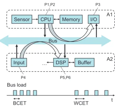
The application A1 consists of a sensor that sends periodically bursts of data to the CPU, which stores them in the memory using a task P1. These data are processed by the CPU using a task P2, with a worst case
Bus load
t
BCET WCET
Sensor CPU Memory I/O
Input DSP Buffer A1 A2 Bus … P1,P2 P3 P5,P6 P4
Figure 1: Interference of two applications on a shared communication re-source.
execution time WCET and a best case execution time BCET. The processed data are transmitted via the shared bus to a hardware input/output device that is running taskP3. We suppose that the CPU uses a preemptive fixed-priority scheduling policy, where P1 has the highest priority. The maximal workload on the CPU is obtained whenP2 continuously uses the WCET and when the sensor simultaneously submits data. There is a second streaming application A2 that receives real-time data in equidistant packets via the Input interface. The Input interface is running taskP4 to send the data to a digital signal processor (DSP) for processing with taskP5. The processed packets are then transferred to a playout buffer and task P6 periodically removes packets from the buffer, e.g. for playback. We suppose that the bus uses a FCFS (first come first serve) scheme for arbitration. As the bus transactions from the applicationsA1 and A2 interfere on the common bus, there will be a jitter in the packet stream received by the DSP that eventually may lead to an undesirable buffer overflow or underflow. It is now interesting to note that the worst case situation in terms of jitter occurs if the processing in A1 uses its BCET, as this leads to a blocking of the bus for a long time period. Therefore, the worst case situation for the CPU load leads to a best case for the bus, and vice versa.
In case of more realistic situations, there will be simultaneous resource sharing on the computing and communication resources, there may be
dif-ferent protocols and scheduling policies on these resources, there may be a distributed architecture using interconnected sub-networks, and there may be additional non-determinism caused by unknown input patterns and data. It is the purpose of performance analysis to determine the timing and mem-ory properties of such systems.
1.2 Basic Terms
As a starting point to the analysis of timing and performance of embedded systems, it is very useful to clarify a few basic terms. Very often, the tim-ing behavior of an embedded system can be described by the time interval between a specified pair of events. For example, the instantiation of a task, the occurrence of a sensor input, or the arrival of a packet could be a start event. Such events will be denoted asarrival events. Similar, the finishing of an application or a part of it can again be modeled as an event, denoted as finishing event. In case of a distributed system, the physical location of the finishing event may not be equal to that of the corresponding arrival event and the processing may require the processing of a sequence or set of tasks, and the use of distributed computing and communication resources. In this case, we talk about end-to-end timing constraints. Note that not all pairs of events in a system are necessarily critical, i.e. have deadline requirements.
An embedded system processes the data associated with arrival events. The timing of computations and communications within the embedded sys-tem may depend on the input data (because of data dependent behavior of tasks) and on the arrival pattern. In case of a conservative resource shar-ing strategy, such as the time triggered architecture (TTA), the interference between these tasks is removed by applying a static sharing strategy. If the use of shared resources is controlled by dynamic policies, all activities may interact with each other and the timing properties influence each other. As has been shown in the previous section, it is necessary to distinguish between the following terms:
• Worst case and best case: The worst case and the best case are the maximal and minimal time interval between the arrival and finishing events under all admissible system and environment states. The execu-tion time may vary largely, due to different input data and interference between concurrent system activities.
• Upper and lower bounds: Upper and lower bounds are quantities that bound the worst case and best case behavior. These quantities are usually computed off-line, i.e. not during the run-time of the system.
• Statistical measures: Instead of computing bounds on the worst case and best case behavior, one may also determine a statistical
character-ization of the run-time behavior of the system, e.g. expected values, variances and quantiles.
In the case of real-time systems, we are particularly interested in upper and lower bounds. They are used in order to verify statically, whether the system meets its timing requirements, e.g. deadlines.
In contrast to the end-to-end timing properties, the termperformance is less well defined. Usually, it refers to a mixture of the achievable deadline, the delay of events or packets, and of the number of events that can be processed per time unit (throughput). There is a close relation between the delay of individual packets or events, the necessary memory in the embedded system and the throughput, i.e. the required memory is proportional to the product of throughput and delay. Therefore, we will concentrate on the delay and memory properties in later sections.
Several methods do exist, such as analysis, simulation, emulation and implementation, in order to determine or approximate the above quantities. Besides analytic methods based on formal models, one may also consider simulation, emulation or even implementation. All the latter possibilities should be used with care as only a finite set of initial states, environment behaviors and execution traces can be considered. As is well known, the corner cases that lead to a worst case or best case execution time are usually not known, and thus incorrect results may be obtained. The huge state space of realistic system architectures makes it highly improbable that the critical instances of the execution can be determined without the help of analytical methods.
In order to understand the requirements for performance analysis meth-ods in distributed embedded systems, we will classify possible causes for a large difference between the worst case and best case or between the upper and lower bounds.
• Non-determinism and interference: Let us suppose that there is only limited knowledge about the environment of the embedded system, for example, about the time when external events arrive or about their input data. In addition, there is interference of computation and communication on shared resources such as CPU, memory, bus or network. Then, we will say that the timing properties are non-deterministic with respect to the available information. Therefore, there will be a difference between the worst case and the best case behavior as well as between the associated bounds. An example may be that the execution time of a task may depend on its input data. Another example is the communication of data packets on a bus in case of an unknown interference.
• Limited analyzability: If there is complete knowledge about the whole system, then the behavior of the system is determined. Nevertheless,
it may be that because of the system complexity, there is no feasible way of determining close upper and lower bounds on the worst case and best case timing, respectively.
As a result of this discussion, we understand that methods to analyze the performance of distributed embedded system must be (a) correct in that they determine valid upper and lower bounds and (b) accurate in that the determined bounds are close to the actual worst case and best case.
In contrast to other chapters of the handbook, we will concentrate on the interaction between thetask level of an embedded system and thedistributed operation. We suppose that the whole application is partitioned into tasks and threads. Therefore, the task level refers to operating system issues like scheduling, memory management and arbitration of shared resources. In addition, we are faced with applications that run on distributed resources. The corresponding layer contains methods of distributed scheduling and networking. On this level of abstraction we are interested in end-to-end timing and performance properties.
1.3 Role in the Design Process
One of the major challenges in the design process of embedded systems is to estimate essential characteristics of the final implementation early in the design. This can help in making important design decisions before investing too much time in detailed implementations. Typical questions faced by a designer during a system-level design process are: Which functions should be implemented in hardware and which in software (partitioning)? Which hardware components should be chosen (allocation)? How should the dif-ferent functions be mapped onto the chosen hardware (binding)? Do the system-level timing properties meet the design requirements? What are the different bus utilizations and which bus or processor acts as a bottleneck? Then there are also questions related to the on-chip memory requirements and off-chip memory bandwidth.
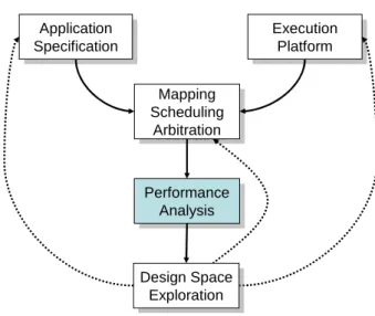
Typically, the performance analysis or estimation is part of the design space exploration, where different implementation choices are investigated in order to determine the appropriate design trade-offs between the different conflicting objectives, for an overview see [20]. Following Figure 2, the estimation of system properties in an early design phase is an essential part of the design space exploration. Different choices of the underlying system architecture, the mapping of the applications onto this architecture, and the chosen scheduling and arbitration schemes will need to be evaluated in terms of the different quality criteria.
In order to achieve acceptable design times though, there is a need for automatic or semi-automatic (interactive) exploration methods. As a result, there are additional requirements for performance analysis if used for design
Application Specification Application
Specification ExecutionPlatform Execution Platform Mapping Scheduling Arbitration Mapping Scheduling Arbitration Performance Analysis Performance Analysis Design Space Exploration Design Space Exploration
Figure 2: Relation between design space exploration and performance anal-ysis.
space exploration, namely (a) the simple reconfigurability with respect to architecture, mapping and resource sharing policies, (b) a short analysis time in order to be able to test many different choices in a reasonable time frame and (c) the possibility to cope with incomplete design information, as typically the lower layers are not designed or implemented (yet).
Even if the design space exploration as described above is not a part of the chosen design methodology, the performance analysis is often part of the development process of software and hardware. In embedded system design, the functional correctness is validated after each major design step using simulation or formal methods. If there are non-functional constraints such as deadline or throughput requirements, they need to be validated as well and all aspects of the design representation related to performance become ’first class citizens’.
Finally, performance analysis of the whole embedded system may be done after completion of the design, in particular if the system is operated under hard real-time conditions where timing failures lead to a catastrophic situation. As has been mentioned above, performance simulation is not appropriate in this case because the critical instances and test patterns are not known in general.
1.4 Requirements
Based on the discussion above, one can list some of the requirements that a methodology for performance analysis of distributed embedded systems must satisfy.
• Correctness: The results of the analysis should be correct, i.e. there exist no reachable system states and feasible reactions of the system environment such that the calculated bounds are violated.
• Accuracy: The lower and upper bounds determined by the perfor-mance analysis should be close to the actual worst case and best case timing properties.
• Embedding into the design process: The underlying performance model should be sufficiently general to allow the representation of the appli-cation (which possibly uses different specifiappli-cation mechanisms), of the environment (periodic, aperiodic, bursty, different event types), of the mapping including the resource sharing strategies (preemption, pri-orities, time-triggered) and of the hardware platform. The method should seamlessly integrate into the functional specification and de-sign methodology.
• Short analysis time: Especially, if the performance analysis is part of a design space exploration, a short analysis time is important. In addition, the underlying model should allow for reconfigurability in terms of application, mapping and hardware platform.
As distributed systems are heterogeneous in terms of the underlying ex-ecution platform, the diverse concurrently running applications, and the dif-ferent scheduling and arbitration policies used, modularity is a key require-ment for any performance analysis method. We can distinguish between several composition properties:
• Process Composition: Often, events need to be processed by several consecutive application tasks. In this case, the performance analysis method should be modular in terms of this functional composition.
• Scheduling Composition: Within one implementation, different scheduling methods can be combined, even within one computing resource (hierarchal scheduling); the same property holds for the scheduling and arbitration of communication resources.
• Resource Composition: A system implementation can consist of differ-ent heterogeneous computing and communication resources. It should be possible to compose them in a similar way as processes and schedul-ing methods.
• Building Components: Combinations of processes, associated schedul-ing methods and architecture elements should be combined into com-ponents. This way, one could associate a performance component to a combined hardware/OS/software module of the implementation, that
exposes the performance requirements but hides internal implementa-tion details.
It should be mentioned that none of the approaches known to date are able to satisfy all of the above mentioned criteria. On the other hand, depending on the application domain and the chosen design approach, not all of the requirements are equally important. The next section summarizes some of the available methods and in section 3 one available method is described in more detail.
2
Approaches to Performance Analysis
In this survey, we select just a few representative and promising approaches that have been proposed for the performance analysis of distributed embed-ded systems.
2.1 Simulation Based Methods
Currently, the performance estimation of embedded systems is mainly done using simulation or trace-based simulation. Examples of available ap-proaches and software support provides the SystemC initiative, see e.g. [16, 8], that is supported by tools from companies like Cadence (nc-systemc) and Synopsys (System Studio). In simulation-based methods, many dy-namic and complex interactions can be taken into account whereas analytic methods usually have to stick to a restrictive underlying model and suffer from limited scope. In addition, there is the possibility to match the level of abstraction in the representation of time to the required degree of accuracy. Examples for these different layers are cycle-accurate models, e.g. those used in the simulation of processors [3], up to networks of discrete event components that can be modeled in SystemC.
In order to determine timing properties of an embedded system, a simu-lation framework not only has to consider the functional behavior but also requires a concept of time and a way of taking into account properties of the execution platform, of the mapping between functional computation and communication processes and elements of the underlying hardware, and of resource sharing policies (as usually implemented in the operating system or directly in hardware). This additional complexity leads to higher com-putation times, and performance estimation quickly becomes a bottleneck in the design. Besides, there is a substantial set-up effort necessary if the mapping of the application to the underlying hardware platform changes, for example in order to perform a design space exploration.
The fundamental problem of simulation-based approaches to perfor-mance estimation is the insufficient corner case coverage. As shown in the example in Fig. 1, the subsystem corner case (high computation time ofA1)
does not lead to the system corner case (small computation time ofA1). De-signers must provide a set of appropriate simulation stimuli in order to cover all the corner cases that exist in the distributed embedded system. Failures of embedded systems very often relate to timing anomalies that happen in-frequently and therefore, are almost impossible to discover by simulation. In general, simulation provides estimates of the average system performance but does not yield worst-case results and can not determine whether the system satisfies required timing constraints.
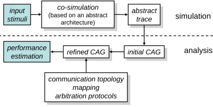
The approach taken by Lahiri et al. [9] combines performance simulation and analysis by a hybrid trace-based methodology. It is intended to fill the gap between pure simulation that may be too slow to be used in a design space exploration cycle, and analytic methods that are often to restricted in scope and not accurate enough. The approach as described concentrates on communication aspects of a distributed embedded system. The performance estimation is partitioned into several stages, see Figure 3:
input stimuli co-simulation (based on an abstract architecture) co-simulation (based on an abstract architecture) abstract trace abstract trace initial CAG initial CAG communication topology mapping arbitration protocols communication topology mapping arbitration protocols refined CAG refined CAG performance estimation simulation analysis
Figure 3: A hybrid method for performance estimation, based on simulation and analytic methods.
• Stage 1: An initial co-simulation of the whole distributed system is performed. The simulation not only covers functional aspects (pro-cessing of data) but also captures the communication in an abstract manner, i.e. in form of events, tokens or abstract data transfers. The resulting set of traces cover essential characteristics of computation and communication but do not contain data information anymore. Here, we do not take into account resource sharing such as different arbitration schemes and access conflicts. The output of this step is a timing inaccurate system execution trace.
• Stage 2: The traces from stage 1 are transformed into an initial Com-munication Analysis Graph (CAG). One can omit unnecessary details
(values of the data communicated, only the size might be important here, etc.) and bursts of computation/communication events might be clustered by identifying only start and end times of these bursts.
• Stage 3: A communication topology is chosen, the mapping of the abstract communications to paths in the communication architecture (network, bus, point-to-point links) is specified and finally, the corre-sponding arbitration protocols are chosen.
• Stage 4: In the analytic part of the whole methodology, the Commu-nication Analysis Graph from stage 2 is transformed and refined using the information in stage 3. It now captures the computation, com-munication and synchronization as seen on the target system. To this end, the initial CAG is augmented to incorporate the various latencies and additional computations introduced by moving from an abstract communication model to an actual one.
The resulting CAG can then be analyzed in order to estimate the sys-tem performance, determine critical paths, and collect various statis-tics about the computation and communication components.
The above approach still suffers from several disadvantages. All traces are the result of a simulation, and the coverage of corner cases is still limited. The underlying representation is a complete execution of the application in form of a graph which may be of prohibitive size. The effect of the transfor-mations applied in order to (a) reduce the size of the Communication Anal-ysis Graph and to (b) incorporate the concrete communication architecture are not formally specified. Therefore, it is not clear what the final analysis results represent. Finally, because of the separation between the functional simulation and the non-functional analysis, no feedback is possible. For example, a buffer overflow because of a sporadic communication overload situation may lead to a difference in the functional behavior. Nevertheless, the described approach blends two important approaches to performance estimation, namely simulation and analytic methods and makes use of the best properties of both worlds.
2.2 Holistic Scheduling Analysis
There is a large body of formal methods available for scheduling of shared computing resources, for example fixed-priority, rate-monotonic, earliest deadline first scheduling, time triggered policies like TDMA or round-robin and static cyclic scheduling. From the worst case execution time of indi-vidual tasks, the arrival pattern of activation and the particular scheduling strategy, one can analyze in many cases the schedulability and worst case response times, see e.g. [4]. Many different application models and event patterns have been investigated such as sporadic, periodic, jitter, and bursts.
There exists a large number of commercial tools that allow for this ’one-model approach’ the analysis of quantities like resource load and response times. In a similar way, network protocols are increasingly supported by analysis and optimization tools.
The classical scheduling theory has been extended towards distributed systems where the application is executed on several computing nodes and the timing-properties of the communication between these nodes can not be neglected. The seminal work of Tindell and Clark [22] combined fixed prior-ity preemptive scheduling at computations nodes with TDMA scheduling on the interconnecting bus. These results are based on two major achievements:
• The communication system (in this case, the bus), was handled in a similar way than the computing nodes. Because of this integration of process and communication scheduling, the method was called a holistic approach to the performance analysis of distributed real-time systems.
• The second contribution was the analysis of the influence of the release jitter on the response time, where the release jitter denotes the worst case time difference between the arrival (or activation) of a process and its release (making it available to the processor). Finally, the release jitter has been linked to the message delay induced by the the communication system.
This work was improved in terms of accuracy by Wolf [25] by taking into account correlations between arrivals of triggering events. In the meantime, many extensions and applications have been published based on the same line of thoughts. Other combinations of scheduling and arbitration policies have been investigated, such as Controller Area Networks (CAN) [21], and more recently, the FlexRay protocol [11]. The latter extension opens the holistic scheduling methodology to mixed event triggered and time triggered systems where the processing and communication is driven by the occurrence of events or the advance of time, respectively.
Nevertheless, it must be noted that the holistic approach does not scale to general distributed architectures in that for every new kind of application structure, sharing of resources and combination thereof, a new analysis needs to be developed. In general, the model complexity grows with the size of the system and the number of different scheduling techniques. In addition, the method is restricted to the classical models of task arrival patterns such as periodic, or periodic with jitter.
2.3 Compositional Methods
Three main problems arise in the case of complex distributed embedded systems: Firstly, the architecture of such systems, as already mentioned, is
highly heterogeneous—the different architectural components are designed assuming different input event models and use different arbitration and re-source sharing strategies. This makes any kind ofcompositional performance analysis difficult. Secondly, applications very often rely on a high degree of concurrency. Therefore, there are multiple control threads, which addition-ally complicate timing analysis. And thirdly, we can not expect that an embedded system only needs to process periodic events where to each event a fixed number of bytes is associated. If for example the event stream rep-resents a sampled voice signal, then after several coding, processing and communication steps, the amount of data per event as well as the timing may have changed substantially. In addition, stream based systems often also have to process other event streams that are sporadic or bursty, e.g. they have to react to external events or deal with best-effort traffic for cod-ing, transcription or encryption. There are only a few approaches available that can handle such complex interactions.
One approach is based on a unifying model of different event patterns in the form of arrival curves as known from the networking domain, see [18, 17]. The proposed real-time calculus represents the resources and their process-ing or communication capabilities in a compatible manner and therefore, allows for a modular hierarchical scheduling and arbitration for distributed embedded systems. The approach will be explained in the next section in some more detail.
Richter et al. propose in [14, 13, 12] a method that is based on classical real-time scheduling results. They combine different well known abstrac-tions of event task arrival patterns and provide additional interfaces between them. The approach is based on the following principles:
• The main goal is to make use of the very successful results in real-time scheduling, in particular for sharing a single processor or a single communication link, see e.g. [4, 15]. For a large class of scheduling and arbitration policies and a set of arrival patterns (periodic, periodic with jitter, sporadic and bursty), upper and lower bounds on the response time can be determined, i.e. the time difference between the arrival of a task and its finishing time. Therefore, the abstraction of a task of the application consists of a triggering event stream with a certain arrival pattern, the WCET worst case execution time) and BCET (best case execution time) on the resource. Several tasks can be mapped onto a single resource. Together with the scheduling policy, one can obtain for each task the associated lower and upper bound of the response time. In a similar way, communication and shared busses can be handled.
• The application model is a simple concatenation of several tasks. The end-to-end delay can now be obtained by adding the individual con-tributions of the tasks; the necessary buffer memory can simply be computed taking into account the initial arrival pattern.
• Obviously, the approach is feasible only if the arrival patterns fit the few basic models for which results on computing bounds on the re-sponse time are available. In order to overcome this limitation, two types of interfaces are defined:
– EMIF: Event Model Interfaces are used in the performance analy-sis only. They perform a type conversion between certain arrival patterns, i.e. they change the mathematical representation of event streams.
– EAF: Event Adaptation Functions need to be used in cases where there exists no EMIF. In this case, the hardware/software imple-mentation must be changed in order to make the system analyz-able, e.g. by adding playout buffers at appropriate locations. In addition, a new set of six arrival patterns was defined [13] which is more suitable for the proposed type conversion using EMIF and EAF, see Figure 4. periodic t T ti ti+1 ti+1
–
ti= T periodic w/ jitter t T ti ti= i ⋅T + ϕi + ϕ0admissible occurrence of event
J 0 >ϕi> J J > T periodic w/ burst t T ti ti= i ⋅T + ϕi + ϕ0 J 0 >ϕi> J J > T ti+1
–
ti> dFigure 4: Some arrival patterns of tasks that can be used to characterize properties of event streams in [13]. T,J and ddenote the period, jitter and minimal interarrival time, respectively. φ0 denotes a constant phase shift.
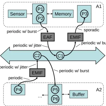
In Figure 5, the example of Fig. 1 is extended by adding the tasks P1 to P6, appropriate arrival patterns (event stream abstractions) and EMIF/EAF interfaces. For example, we suppose that there is an analy-sis method for the bus arbitration scheme available that requires ’periodic with jitter’ as the input model. As the transformation from ’periodic with burst’ requires an Event Adaptation Function, the implementation must be changed to accommodate a buffer that smoothens the bursts. From ’pe-riodic’ to ’periodic with jitter’, one can construct a lossless Event Model
Interface simply by setting the jitterJ = 0. There is another interface be-tween communicationC1 and taskP3 that converts the bursty output of the bus to a sporadic model. Now, one can apply performance analysis methods to all of the components. As a result, one may determine the minimal buffer size and an appropriate scheduling policy for the DSP such that no overflow or underflow occurs. Sensor Memory Buffer A1 A2 P1 P2 P3 P5 P4 C1 C2 periodic w/ burst periodic w/ jitter periodic periodic w/ jitter periodic w/ burst sporadic periodic w/ burst P6 EAF EMIF … EMIF
Figure 5: Example of event stream interfaces for the example in Fig. 1. Several extensions have been worked out, e.g. in order to deal with cyclic non-functional dependencies and to generalize the application model. Nevertheless, when comparing the requirements for a modular performance analysis, the approach has some inherent drawbacks. EAFs are caused by the limited class of supported event models and the available analysis meth-ods. The analysis method enforces a change in the implementation. Fur-thermore, the approach is not modular in terms of the resources, as their service is not modeled explicitly. For example, if several scheduling policies need to be combined in one resource (hierarchical scheduling), then for each new combination an appropriate analysis method must be developed. In this way, the approach suffers from the same problem as the ’holistic ap-proach’ described earlier. In addition, one is bound to the classical arrival patterns that are not sufficient in case of stream processing applications. Other event models need to be converted with loss in accuracy (EMIF) or the implementation must be changed (EAF).
3
The Performance Network Approach
This section describes an approach to the performance analysis of embed-ded systems that is influenced by the worst-case analysis of communication networks. The network calculus as described in [2] is based on [7] and uses (max,+)-algebra to formulate the necessary operations. The network calcu-lus is a promising analysis methodology as it is designed to be modular in various respects and as the representation of event (or packet) streams is not restricted to the few classes mentioned in the previous section. In [19, 18], the method has been extended to the real-time calculus in order to deal with distributed embedded systems by combining computation and commu-nication. Because of the detailed modeling of the capability of the shared computing and communication resources as well as the event streams, a high accuracy can be achieved, see [6]. The following sections serve to explain the basic approach.
In addition, the main performance analysis method is not bound to the use of the real-time calculus. Instead, any suitable abstraction of event streams and resource characterization is possible. Only the actual computa-tions that are done within the components of the performance network need to be changed appropriately.
3.1 Performance Network
In functional specification and verification, the given application is usually decomposed into components that are communicating via event interfaces. The properties of the whole system are investigated by combining the behav-ior of the components. This kind of representation is common in the design of complex embedded systems and is supported by many tools and stan-dards, e.g. UML. It would be highly desirable if the performance analysis follows the same line of thinking as it could be integrated into the usual de-sign methodology easily. Considering the discussion in the previous sections, we can identify two major additions that are necessary:
• Abstraction: Performance analysis is interested in making statements about the timing behavior not just for one specific input characteri-zation but for a larger class of possible environments. Therefore, the concrete event streams that flow between the components must be represented in an abstract way. As an example, we have seen their characterization by ’periodic’ or ’sporadic with jitter’. The same way, the non-functional properties of the application and the resource shar-ing mechanisms must be modeled appropriately.
• Resource Modeling: In comparison to functional validation, we need to model the resource capabilities and how they are changed by the workload of tasks or communication. Therefore, in contrary to the
approaches described before, we will model the resources explicitly as ’first class citizens’ of the approach.
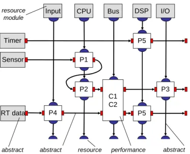
As an example of a performance network, let us look again at the sim-ple examsim-ple from Fig. 1 and Fig. 5. In Figure 6, we see a corresponding performance network. Because of the simplicity of the example, not all the modeling possibilities can be shown.
On the left hand side, you see theabstract inputwhich models the sources of the event streams that trigger the tasks of the applications: ’Timer’ rep-resents the periodic instantiation of the task that reads out the buffer for playback, ’Sensor’ models the periodic bursty events from the sensor and ’RT data’ denotes the real-time data in equidistant packets via the Input interface. The associatedabstract event streams are transformed by the per-formance components. On the top, you can see the resource modules that model the service of the shared resources, e.g. the Input, CPU, Bus, CPU and I/O component. Theabstract resource streams (vertical direction) in-teract with the event streams on the performance modules and performance components. Theresource interfaces at the bottom represent the remaining resource service that is available to other applications that may run on the execution platform.
Theperformance components represent (a) the way how the timing prop-erties of input event streams are transformed to timing propprop-erties of output event streams and (b) the transformation of the resources. Of course, these components can be hierarchically grouped into larger components. The way how the performance components are grouped and their transfer function reflect the resource sharing strategy. For example,P1 andP2 are connected serially in terms of the resource stream and therefore, they model a fixed priority scheme with the high priority assigned to taskP1. If the bus imple-ments FCFS strategy or a TTP, the transfer function ofC1/C2 needs to be determined such that the abstract representations of the event and resource stream are correctly transformed.
3.2 Variability Characterization
The timing characterization of event and resource streams is based on Vari-ability Characterization Curves (VCC) which substantially generalize the classical representations such as sporadic or periodic. As the event streams propagate through the distributed architecture, their timing properties get increasingly complex and the standard patterns can not model them with appropriate accuracy.
The event streams are described using arrival curves ¯αu(∆), ¯αl(∆) ∈ R≥0, ∆ ∈ R≥0 which provide upper and lower bounds on the number of
events in any time interval of length ∆. In particular, there are at most ¯
Input CPU Bus DSP P1 Sensor RT data I/O P2 P3 P4 P5 Timer P5 C1 C2 resource module abstract input abstract event stream abstract resource stream performance component resource interface
Figure 6: A simple performance network related to the example in Fig. 1 t≥0.
In a similar way, the resource streams are characterized using service functions βu(∆), βl(∆) ∈ R≥0, ∆ ∈ R≥0 provide upper and lower bounds
on the available service in any time interval of length ∆. The unit of ser-vice depends on the kind of the shared resource, for example instructions (computation) or bytes (communication).
Note that as defined above, the VCC’s ¯αu(∆) and ¯αl(∆) are expressed
in terms of events (this is marked by a bar on their symbol), while the VCC’s βu(∆) and βl(∆) are expressed in terms of workload/service. A
method to transform event-based VCC’s to workload/resource-based VCC’s and vice-versa is presented later in this chapter. All calculations and trans-formations presented here are valid both with only event-based or with only workload/resource-based VCC’s, but in this chapter mainly the event-based formulation is used.
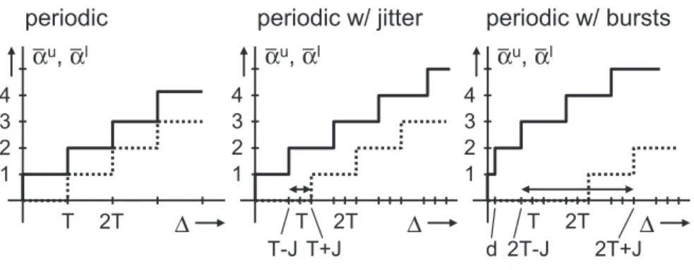
Figure 7 shows arrival curves that specify the basic classical models shown in Fig. 4. Note that in case of sporadic patterns, the lower arrival curves are 0. In a similar way, Figure 8 shows a service curve of a simple TDMA bus access with periodT, bandwidth b and slot intervalτ.
Note that arrival curves can be approximated using linear approxima-tions, i.e. a piecewise linear function. Moreover, there are of course finite representations of the arrival and service curves, for example by decompos-ing them into an irregular initial part and a periodic part.
Where do we get the arrival and service functions from, e.g. those char-acterizing a processor (CPU in Fig. 6), or an abstract input (Sensor in
∆ 1 2 3 4 ∆ αu, αl 1 2 3 4 ∆ 1 2 3 4
periodic periodic w/ jitter periodic w/ bursts
T 2T T 2T T-J T+J 2T+J T 2T 2T-J d αu, αl αu, αl
Figure 7: Basic arrival functions related to the patterns described in Fig. 4.
t T τ bandwidth b ∆ βu, βl T 2T T-τ τ bτ
Figure 8: Example of a service curve that describes a simple TDMA proto-col.
Fig. 6).
• Pattern: In some cases, the patterns of the event or resource stream are known, e.g. bursty, periodic, sporadic and TDMA. In this case, the functions can be constructed analytically, see e.g. Figs. 7, 8.
• Trace: In case of unknown arrival or service patterns, one may use a set of traces and compute the envelope. This can be done easily by using a sliding window of size ∆ and determining the maximum and minimum number of events (or service) within the window.
• Data Sheets: In other cases, one can derive the curves by deriving the bounds from the characteristic of the generating device (in terms of the arrival curve) or the hardware component (in case of service curve).
The performance components transform abstract event and resource streams. But so far, the arrival curve is defined in terms of events per time interval whereas the service curve is given in terms of service per time interval. One possibility to overcome this gap is to define the concept of
workload curves that connect the number of successive events in an event stream and the maximal or minimal workload associated. They capture the variability in execution demands.
The upper and lower workload curveγu(e),γl(e)∈R≥0 denote the
max-imal and minmax-imal workload on a specific resource for any sequence ofe con-secutive events. If we have these curves available, then we can easily deter-mine upper and lower bounds on the workload that an event stream imposes in any time interval of length ∆ on a resource as αu(∆) =γu(¯αu(∆)) and
αl(∆) = γl(¯αl(∆)), respectively. And analogously, ¯βu(∆) = γl−1(βu(∆))
and ¯βl(∆) =γu−1(βl(∆)). As in the case of the arrival and service curves,
it appears the question, where the workload curves can come from. A selec-tion of possibilities is given below.
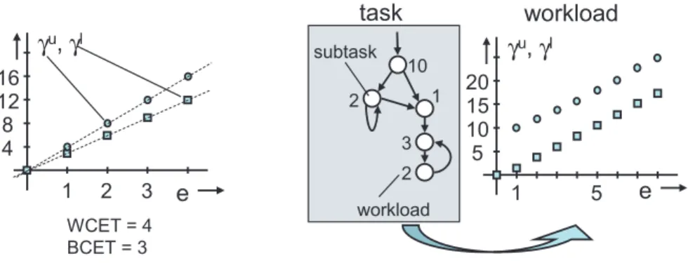
• WCET and BCET: The simplest possibility is to (a) assume that each event of an event stream triggers the same task and (b) that this task has a given worst case and best case execution time determined by other methods. An example of an associated workload curve is given in Fig. 9. The same holds for communication events also.
• Application Modeling: The above method models the fact that not all events lead to the same execution load (or number of bits) by simply using upper and lower bounds on the execution time. The accuracy of this approach can be substantially improved, if characteristics of the application are taken into account, e.g. (a) distinguishing between dif-ferent event types each one triggering a difdif-ferent task and (b) modeling that it is not possible that many consecutive events all have the WCET (or BCET). This way, one can model correlations in event streams, see [10]. Fig. 9 represents on the right hand side a simple example where a task is refined into a set of subtasks. At each incoming event, a subtask generates the associated workload and the program branches to one of its successors.
• Trace: As in the case of arrival curves, we can use a given trace and re-port the workloads associated to each event, e,g, by simulation. Based on this information, we can easily compute the upper and lower enve-lope.
A more fine-grained modeling of an application is possible also, e.g. by taking into account different event types in event streams, see [23]. By the same approach, it is also possible to model more complex task models, e.g. a task with different production and consumption rates of events or tasks with several event inputs, see [24]. Moreover, the same modeling holds for the load on communication links of the execution platform also.
In order to construct a scheduling network according to Fig. 6, we still need to take into account the resource sharing strategy.
e γu, γl 4 8 12 16 1 2 WCET = 4 BCET = 3 3 e γu, γl 5 10 15 20 1 5 10 2 2 1 3 subtask workload task workload
Figure 9: Two examples of modeling the relation between incoming events and the associated workload on a resource. The left hand side shows a simple modeling in terms of the WCET and BCET of the task triggered by an event. The right hand side models the workload generated by a task through a finite state machine. The workload curves can be constructed by considering the maximum or minimum weight paths withetransitions.
3.3 Resource Sharing and Analysis
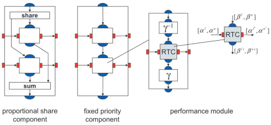
In Fig. 1, we see for example that the performance modules associated to tasks P1 and P2 are connected serially. This way, we can model a pre-emptive fixed priority resource sharing strategy as P2 only gets the CPU resource that is left after the workload of P1 has been served. Other re-source sharing strategies can be modeled as well, see e.g. Fig. 10 where in addition a proportional share policy is modeled on the left. In this case, a fixed portion of the available resource (computation or communication) is associated to each task. Other sharing strategies are possible also, such as FCFS ([2]).
In the same Fig. 10, we also see how the workload characterization as described in the last section is used to transform the incoming arrival curve into a representation that talks about the workload for a resource. After the transformation of the transformation of the incoming stream by a block called RTC (real-time-calculus), the inverse workload transformation may be done again in order to characterize the stream by means of events per time interval. This way, the performance modules can be freely combined as their input and output representations match.
We still need to describe how a single workload stream and resource stream interact on a resource. The underlying model and analysis very much depends on the underlying execution platform. As a common example, we suppose that the events (or data packets) corresponding to a single stream are stored in a queue before being processed, see Fig. 11. The same model is used for computation as well as for communication resources. It matches
fixed priority component share sum proportional share component RTC performance module ] , [ l u α α ] , [ l u β β ] , [ l′ u′ α α ] ' , ' [ l u β β RTC
γ
γ
−1Figure 10: Two examples of resource sharing strategies and their model in the real-time calculus.
well the common structure of operating systems where ready tasks are lined up until the processor is assigned to one of them. Events belonging to one stream are processed in a FCFS manner whereas the order between different streams depends on the particular resource sharing strategy.
service service buffers input streams … resource sharing
Figure 11: Functional model of resource sharing on computation and com-munication resources.
Following this model, one can derive the equations that describe the transformation of arrival and service curves by an RTC module according to Fig. 10, see e.g. [17]:
¯ αu0 = [(¯αu⊗β¯u)®β¯l]∧β¯u ¯ αl0 = [(¯αl®β¯u)⊗β¯l]∧β¯l ¯ βu0 = ( ¯βu−α¯l)®0 ¯ βl0 = ( ¯βl−α¯u)⊗0
Following [1], the operators used are called min-plus/max-plus convolu-tions (f⊗g)(t) = inf 0≤u≤t{f(t−u) +g(u)} (f⊗g)(t) = sup 0≤u≤t {f(t−u) +g(u)}
and min-plus/max-plus deconvolutions
(f®g)(t) = sup
u≥0{f(t+u)−g(u)}
(f®g)(t) = inf
u≥0{f(t+u)−g(u)}
Using these equations, the workload curves, and the characterization of input event and resource streams, we now can determine the characteriza-tions of all event and resource streams in a performance network such as in Fig. 6. From the resulting arrival curves (leaving the network on the right hand side) and service curves (at the bottom), we can compute all the rel-evant information such as the average resource loads, the end-to-end delays and the necessary buffer spaces on the event and packet queues, see Fig. 11. If the performance network contains cycles, then fixed point iterations are necessary.
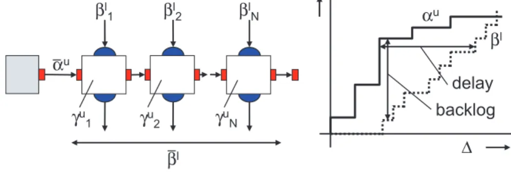
As an example let us suppose that the upper input arrival curve of an event stream is αu(∆). Moreover, the stream is processed by a sequence of
N modules according to the right hand side of Fig. 10 with incoming service curvesβl
i(∆), 1≤i≤N and workload curvesγiu(e). Then we can determine
the maximal end-to-end delay and accumulated buffer space for this stream according to (see [18]) γi−1(W) = sup{e≥0 : γiu(e)≤W} ∀1≤i≤N ¯ βil(∆) =γi−1(βil(∆)) ∀1≤i≤N ¯ βl(∆) = ¯β1l(∆)⊗β¯2l(∆) · · · ⊗β¯Nl (∆) delay ≤ sup ∆≥0 n inf{τ ≥0 : ¯αu(∆)≤β¯l(∆ +τ)} o backlog ≤ sup ∆≥0 {α¯u(∆)−β¯l(∆)}
The curve γ−1(W) denotes the pseudo inverse of a workload curve, i.e. it yields the minimum number of events that can be processed if the service W is available. Therefore, ¯βl
i(∆) is the minimal available service in terms of
events per time interval. It has been shown [2], that the delay and backlog are determined by the accumulated service ¯βl(∆) that can be obtained using
the convolution of all individual services. The delay and backlog can now be interpreted as the maximal horizontal and vertical distance between the arrival and accumulated service curves, respectively, see Figure 12.
βl 1 γu 1 βl 2 γu 2 βl N γu N βl αu ∆ αu βl delay backlog
Figure 12: Representation of the delay and accumulated buffer space com-putation in a performance network.
All the above computations can be implemented efficiently, if appropri-ate representations for the variability characterization curves are used, e.g. piecewise linear, discrete points or periodic.
3.4 Concluding Remarks
Because of the modularity of the performance network, one can easily an-alyze a large number of different mapping and resource sharing strategies for design space exploration. Applications can be extended by adding tasks and performance modules. Moreover, different subsystems can use different kinds of resource sharing without sacrificing the performance analysis.
Of particular interest is the possibility to build a performance component for a combined hardware-software system that describes the performance properties of a whole subsystem. This way, a subcontractor can deliver a HW/SW/OS module that already contains part of the application. The system house can now integrate the performance components of the subsys-tems in order to validate the performance of the whole system. To this end, he does not need to know the details of the subsystem implementations. In addition, a system house can also add an application to the subsystems. Us-ing the resource interfaces that characterize the remainUs-ing available service from the subsystems, its timing correctness can easily be verified.
The performance network approach is correct in the sense that it yields upper and lower bounds on quantities like end-to-end delay and buffer space. On the other hand, it is a worst-case approach that covers all possible corner cases independent of their probability. Even if the deviations from simula-tion results can be small, see e.g. [5], in many cases one is interested in average case behavior of distributed embedded systems also. Therefore,
performance analysis methods as those described in this chapter can be considered to be complementary to the existing simulation based validation methods.
Furthermore, any automated or semi-automated exploration of different design alternatives (design space exploration) could be separated into mul-tiple stages, each having a different level of abstraction. It would then be appropriate to use an analytical performance evaluation framework, such as those described in this chapter, during the initial stages and resort to simu-lation only when a relatively small set of potential architectures is identified.
References
[1] F. Baccelli, G. Cohen, G. Olsder, and J.-P. Quadrat, Synchronization and linearity, John Wiley, Sons, New York, 1992.
[2] J.-Y. Le Boudec and P. Thiran, Network calculus - a theory of deter-ministic queuing systems for the internet, Lecture Notes in Computer Science 2050, Springer Verlag, 2001.
[3] Doug Burger and Todd M. Austin, The simplescalar tool set, version 2.0, SIGARCH Comput. Archit. News25 (1997), no. 3, 13–25.
[4] G.C. Buttazzo,Hard real-time computing systems: Predictable schedul-ing algorithms and applications, Kluwer Academic Publishers, Boston, 1997.
[5] S. Chakraborty, S. K¨unzli, and L. Thiele, A general framework for analysing system properties in platform-based embedded system designs, Proc. 6th Design, Automation and Test in Europe (DATE) (Munich, Germany), March 2003.
[6] S. Chakraborty, S. K¨unzli, L. Thiele, A. Herkersdorf, and P. Sagmeister, Performance evaluation of network processor architectures: Combining simulation with analytical estimation, Computer Networks 41 (2003), no. 5, 641–665.
[7] R.L. Cruz, A calculus for network delay, Part I: Network elements in isolation, IEEE Transactions on Information Theory 37 (1991), no. 1, 114–131.
[8] T. Gr¨otker, S. Liao, G. Martin, and S. Swan,System Design with Sys-temC, Kluwer Academic Publishers, Boston, May 2002.
[9] K. Lahiri, A. Raghunathan, and S. Dey,System-level performance anal-ysis for designing on-chip communication architectures, IEEE Transac-tions on Computer-Aided Design of Integrated Circuits and Systems 20 (2001), no. 6, 768–783.
[10] Alexander Maxiaguine, Simon K¨unzli, and Lothar Thiele, Workload characterization model for tasks with variable execution demand, Design Automation and Test in Europe (DATE) (Paris, France), IEEE Press, February 2004, pp. 1040–1045.
[11] T. Pop, P. Eles, and Z. Peng,Holistic scheduling and analysis of mixed time/event triggered distributed embedded systems, Int. Symposium on Hardware-Software Codesign (CODES), May 1995, pp. 187–192. [12] K. Richter and R. Ernst, Model interfaces for heterogeneous system
analysis, Proc. 6th Design, Automation and Test in Europe (DATE) (Munich, Germany), March 2002, pp. 506 – 513.
[13] K. Richter, D. Ziegenbein, M. Jersak, and R. Ernst,Model composition for scheduling analysis in platform design, Proc. 39th Design Automa-tion Conference (DAC) (New Orleans, LA), ACM Press, June 2002. [14] Kai Richter, Marek Jersak, and Rolf Ernst,A formal approach to mpsoc
performance verification, IEEE Computer36(2003), no. 4, 60–67. [15] J.A. Stankovic, M. Spuri, K. Ramamritham, and G.C. Buttazzo,
Dead-line scheduling for real-time systems: EDF and related algorithms, Kluwer International Series in Engineering and Computer Science, vol. 460, Kluwer Academic Publishers, 1998.
[16] SystemC homepage,http://www.systemc.org.
[17] L. Thiele, S. Chakraborty, M. Gries, and S. K¨unzli, A framework for evaluating design tradeoffs in packet processing architectures, Proc. 39th Design Automation Conference (DAC) (New Orleans, LA), ACM Press, June 2002, pp. 880–885.
[18] L. Thiele, S. Chakraborty, M. Gries, A. Maxiaguine, and J. Greutert, Embedded software in network processors – models and algorithms, Proc. 1st Workshop on Embedded Software (EMSOFT) (Lake Tahoe, CA, USA), Lecture Notes in Computer Science 2211, Springer Verlag, 2001, pp. 416–434.
[19] L. Thiele, S. Chakraborty, and M. Naedele, Real-time calculus for scheduling hard real-time systems, Proc. IEEE International Sympo-sium on Circuits and Systems (ISCAS), vol. 4, 2000, pp. 101–104. [20] Lothar Thiele, Simon K¨unzli, and Eckart Zitzler, A modular design
space exploration framework for embedded systems, IEE Proceedings Computers & Digital Techniques (2004), Special Issue on Embedded Microelectronic Systems.
[21] K. Tindell, A. Burns, and A.J. Wellings, Calculating controller area networks (can) message response times, Control Engineering Practice 3 (1995), no. 8, 1163–1169.
[22] K. Tindell and J. Clark, Holistic schedulability analysis for distributed hard real-time systems, Microprocessing and Microprogramming - Eu-romicro Journal (Special Issue on Parallel Embedded Real-Time Sys-tems) 40(1994), 117–134.
[23] Ernesto Wandeler, Alexander Maxiaguine, and Lothar Thiele, Quan-titative characterization of event streams in analysis of hard real-time applications, 10th IEEE Real-Time and Embedded Technology and Ap-plications Symposium (RTAS), May 2004, pp. 450–459.
[24] Ernesto Wandeler and Lothar Thiele,Abstracting functionality for mod-ular performance analysis of hard real-time systems, Asia South Pacific Design Automation Conference (ASP-DAC), January 2005, (To Ap-pear).
[25] T. Yen and W. Wolf,Performance estimation for real-time distributed embedded systems, IEEE Transaction on Parallel and Distributed Sys-tems 9(1998), no. 11, 1125–1136.
![Figure 4: Some arrival patterns of tasks that can be used to characterize properties of event streams in [13]](https://thumb-us.123doks.com/thumbv2/123dok_us/392096.2543584/14.892.219.679.560.813/figure-arrival-patterns-tasks-characterize-properties-event-streams.webp)