Multitask and transfer learning for multi-aspect data

(1)

Multitask and Transfer Learning for

Multi-Aspect Data

Bernardino Romera Paredes

UCL

A dissertation submitted in partial fulfillment of the requirements for the degree of

(2)

(3)

Abstract

Supervised learning aims to learn functional relationships between inputs and outputs. Multitask learning tackles supervised learning tasks by performing them simultaneously to exploit commonalities between them. In this thesis, we focus on the problem of elim-inating negative transfer in order to achieve better performance in multitask learning. We start by considering a general scenario in which the relationship between tasks is unknown. We then narrow our analysis to the case where data are characterised by a combination of underlying aspects, e.g., a dataset of images of faces, where each face is determined by a person’s facial structure, the emotion being expressed, and the lighting conditions. In machine learning there have been numerous efforts based on multilin-ear models to decouple these aspects but these have primarily used techniques from the field of unsupervised learning. In this thesis we take inspiration from these approaches and hypothesize that supervised learning methods can also benefit from exploiting these aspects. The contributions of this thesis are as follows:

1. A multitask learning and transfer learning method that avoids negative transfer when there is no prescribed information about the relationships between tasks. 2. A multitask learning approach that takes advantage of a lack of overlapping

fea-tures between known groups of tasks associated with different aspects.

3. A framework which extends multitask learning using multilinear algebra, with the aim of learning tasks associated with a combination of elements from different aspects.

4. A novel convex relaxation approach that can be applied both to the suggested framework and more generally to any tensor recovery problem.

Through theoretical validation and experiments on both synthetic and real-world datasets, we show that the proposed approaches allow fast and reliable inferences. Furthermore, when performing learning tasks on an aspect of interest, accounting for secondary as-pects leads to significantly more accurate results than using traditional approaches.

(4)

(5)

Acknowledgments

I would like to thank all those people who have supported me during the last three and a half years. Firstly, thank you to my supervisors, Massimiliano Pontil and Nadia Bianchi-Berthouze. I have been extremely lucky to have benefited from their knowledge, advice, motivation, and openness to consider even the most senseless of my suggestions. Thank you to Hane Aung whose interesting conversations have filled my mind with thoughts both research-related and beyond. I am indebted to Andrew McDonald for his research discussions and conversations, and for proof-reading this thesis. Thanks also to Chris Joyce for giving me the motivation to keep writing, and for diligently proof-reading parts of this thesis. Thanks to Andreas Maurer for sharing his ever-brilliant thoughts and for his contagious enthusiasm for learning theory. Thanks to Luca Baldasarre for his support in the first stages of my PhD. Thanks to the examiners of this thesis, David Barber and Tijl De Bie, as well as Mark Herbster who helped me prepare the viva, for their insightful comments and questions which made this a stronger thesis.

Thank you to the Emo & Pain Group: Aneesha Singh, Harry Griffin, Ana Tajadura, Temi Olugbade, Hongying Meng, and all the others at UCLIC. It has been a pleasure to share all those meals and conversations with you during the years.

I am very thankful to Cha Zhang, who gave me the opportunity to work in an amazing project at Microsoft Research. Thanks also to the people I met there, especially to Piotr Bilinski, Mar González, and Danai Koutra.

Finally, I would like to dedicate this thesis to my family: María del Mar, her parents and mine. Their love and support has been a constant source of encouragement to me during this time.

(6)

(7)

8.2.1. Study of different constraints on tensors and their implications . 158 8.2.2. Developing multilinear optimization methods for large scale data 159 A. Multitask Learning Literature Review: Appendix 161 A.1. MAP derivation of Inverse-Wishart prior on the covariance of the task weight vectors . . . 161

(10)

B.1.1. Covariances . . . 164

B.1.2. Concentration inequalities . . . 164

B.1.3. Rademacher and Gaussian averages . . . 165

B.2. Proofs . . . 167

B.2.1. Multitask learning . . . 167

B.2.2. Transfer learning . . . 171

C. Decoupling of Features: Appendix 179 C.1. Proof of Theorem 5.4.1 . . . 179

D. A New Convex Relaxation for Tensor Completion: Appendix 181 D.1. Minimizing overW . . . 181

D.2. Computation of an Approximated Projection . . . 182

(11)

List of Figures

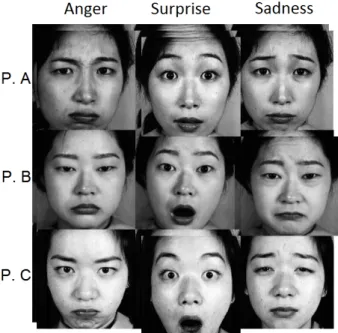
1.1. Samples of a multi-aspect dataset, in which each instance (facial image) is characterised by the identity of the person (P.A, P.B, and P.C), and the emotion being expressed (Anger, Surprise, and Sadness). The images

belong to the JAFFE dataset [124]. . . 19

1.2. Structure of this thesis. . . 25

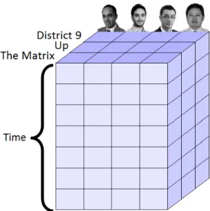
3.1. Example of a tensor modelling the movie preferences of several subjects across time. . . 58

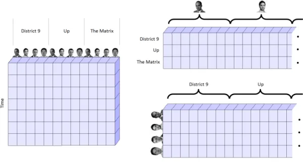
3.2. The three matricizations of the tensor shown in Fig.3.1. . . 59

3.3. CP decomposition of a 3 mode tensor. . . 61

3.4. Tucker decomposition of a 3 mode tensor. . . 63

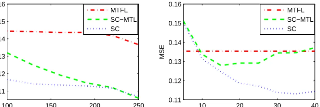
4.1. Multitask error (left) and transfer error (right) vs. number of training tasksT. . . 88

4.2. Multitask error (left) and Transfer error (right) vs. number of atomsK0 used by dictionary-based methods. . . 88

4.3. Multitask error (left) and Transfer error (right) vs. sparsity ratios/K. . 89

4.4. Multiclassification accuracy (among10classes) of RR, MTFL GO-MTL and SC-MTL vs. the number of training instances in the transfer tasks, m. . . . 91

4.5. Transfer error vs. number of tasks T (left) and vs. number of atoms K (right) on the Binary Alphadigits dataset. . . 92

4.6. Dictionaries found by SC-MTL using m = 240 pixels (missing 25% pixels) per image (left) and by Sparse Coding employing all pixels (right). 93 5.1. Synthetic data: Comparison between Ridge Regression (RR), Multitask Feature Learning (MTFL) [8], OrthoMTL, C and OrthoMTL-EN. . . 107

(12)

5.4. Tasks correlation matrix learned by different methods: OrthoMTL-EN (top left), OrthoMTL (top right), MTFL-2G (bottom left), MTFL (bot-tom middle), and Ridge Regression (bot(bot-tom right), Red (resp. blue) denotes high (resp. low) intensity values. . . 109 5.5. JAFFE dataset: Comparison between Bilinear Model and

OrthoMTL-EN in a transfer learning experiment – see text for description. . . 110 5.6. Left: Landmark points and edges used to build the attributes for the

UNBC-McMaster Shoulder Pain Expression Archive (selected accord-ing to Figure shown in [123]). Right: Comparison between Ridge Re-gression (RR), Multitask Feature Learning (MTFL), OrthoMTL-EN, OrthoMTL and OrthoMTL-C on the UNBC-McMaster Shoulder Pain Expression Archive Database. . . 111 6.1. Weight tensor modelling the relation between learning tasks to

recog-nize several AUs from different subjects. . . 117 6.2. The matricizations of the 3-mode tensor shown in Fig.6.1. . . 119 6.3. Tensor of weight vectors and two of its matricizations, illustrating the

scenario when some tasks receive no training instances. . . 121 6.4. Synthetic dataset: Mean Square Error (MSE) comparison between Ridge

Regression (RR), Multitask Feature Learning [8] (MTFL), Matrix Fac-torization MTL (MTL-NC), Convex Multilinear Multitask Learning (MLMTL-C) and Non-convex Multilinear Multitask Learning (MLMTL-N(MLMTL-C). . . 127 6.5. Synthetic dataset: Mean Square Error (MSE) comparison between

Con-vex Multilinear Multitask Learning (MLMTL-C) and three versions of Non-convex Multilinear Multitask Learning (MLMTL-NC) (having dif-ferent values for the ranks). . . 129 6.6. Restaurant & Consumer Dataset: Mean Square Error (MSE)

compari-son between Ridge Regression (RR), Grouped Ridge Regression (GRR), Multitask Feature Learning (MTFL) Grouped Multitask Feature Learn-ing (GMTFL), Matrix Factorization MTL (MTL-NC), Grouped Matrix Factorization (GMTL-NC), MTL Convex Multilinear Multitask Learn-ing C) and Non-convex Multilinear Multitask LearnLearn-ing (MLMTL-NC). . . 130

(13)

6.7. Shoulder Pain database: Mean Square Error (MSE) comparison be-tween Grouped Ridge Regression (GRR), Grouped Multitask Feature Learning (GMTFL), Matrix Trace Norm Regularization (GMTL-NC), Convex Multilinear Multitask Learning (MLMTL-C) and Non-Convex Multilinear Multitask Learning (MLMTL-NC). . . 132 6.8. Affect recognition models adapt themselves to operate on new subjects

by means of MLMTL. . . 134 7.1. Illustration of the convex envelope of a functionf on a given setS. . . . 139 7.2. Example, using a2×2×2×2tensor, illustrating that the spectral norm

is not an invariant property across matricizations of a tensor, in contrast to the Frobenius norm. . . 145 7.3. Synthetic dataset: Root Mean Squared Error (RMSE) of tensor trace

norm and the proposed regularizer (left). Running time execution for different sizes of the tensor (right). . . 150 7.4. Root Mean Squared Error (RMSE) of tensor trace norm and the

pro-posed regularizer for ILEA dataset (left) and Ocean video (right). . . 151 7.5. Restaurant & Consumer Dataset: Mean Square Error (MSE)

compar-ison between the three MLMTL methods described in Chapter 6 and 7: non-convex approach, convex approach based on trace norm, and approach based on the convex relaxation developed in Chapter 7. . . . 153

(14)

(15)

List of Tables

6.1. Index of the notation employed in this chapter. . . 118 7.1. Index of the notation employed in this chapter. . . 138

(16)

(17)

1. Introduction

Over the past decade the field of machine learning has undergone major developments, gradually maturing into a prominent area of computer science. This growth has led to more effective and efficient ways to automatically learn properties from data and to tackle different kinds of scenarios where learning is needed.

One of the scenarios which has been well studied is that of learning a set of super-vised learning tasks with the assumption that they are somehow related. A reasonable approach is to learn these tasks at the same time so that the model can leverage the commonalities between them. This strategy is the core of multitask learning (MTL) [34, 33, 187, 19] and transfer learning (TL) [47, 110, 157, 164, 176]. MTL consists of learning tasks simultaneously, taking advantage of their commonalities, so that the accuracy of each task is increased, whereas in TL, knowledge is gained from a set of source tasks to improve the accuracy of new tasks. These frameworks have successfully been applied in many different scenarios, often providing improved performance over single task learning. Furthermore, when the data available for each task is scarce, single task learning may not be a valid alternative, as there are uniform lower bounds on the performance of single task learning, e.g. see [129].

One significant problem within MTL and TL is negative transfer. In a survey carried out on transfer learning [157], the authors pointed out both the importance of control-ling negative transfer, and the little attention it has received. Negative transfer occurs whenever these frameworks not only fail to improve performance, but actually reduce it. An obvious example would be the naive application of multitask learning to a scenario in which tasks are not related in any way. More generally, negative transfer arises when the model used fails to reflect the specific kinds of relationships held among the tasks, making strong, or simply wrong, assumptions. Thus, all available information about the relationships between tasks should be used whenever possible.

In our research we follow an incremental approach regarding the information available about how tasks are related. Our research starts by studying negative transfer in the broad case where nothing is known about the relationships between tasks. In this

(18)

sce-nario, there may be closely related groups of tasks, as well as tasks which are not related at all. To avoid negative transfer, the model should not presume relations between tasks, however it should be able to positively transfer knowledge between tasks that are re-lated.

In a second stage of this research, we consider using extra information that may be use-ful to uncover the relationships between tasks. Several approaches based on this key principle have previously been proposed and studied. They target the cases where infor-mation about relationships takes the form of clusters and hierarchies [58, 99, 201, 225]. Nevertheless, there are important real cases when these structures lack the necessary ex-pressiveness to encode the relationships between tasks. One such instance arises when data can be looked at from several different angles. In this case, it would be preferable to learn representations of the data that are tailored to the learning tasks at hand, fil-tering out or leveraging other viewpoints of the data. Hereafter, we will refer to those viewpoints as aspects, and to the resultant datasets as multi-aspect datasets. In this the-sis we focus on modelling relationships between tasks in multi-aspect data situations because they appear naturally in many real learning problems, yet they have received little attention.

1.1. Multi-aspect data

Multi-aspect datasets are those composed of instances that can be simultaneously cate-gorized according to different category systems (aspects). Let us consider for example a dataset composed of many images of faces, as in Fig.1.1. Each image is determined by the person who appears in it (aspect 1), the emotion (aspect 2) and perhaps other char-acteristics such as the viewpoint (aspect 3) and the illumination (aspect 4). Multi-aspect datasets are very common, as they arise whenever there are different conditions involved in the data gathering process. A representative example occurs when data are obtained from multiple people, as is the case in many social and medical scientific experiments, and in data gathered by companies about their clients.

In many supervised learning problems only one of those aspects is generally of interest, for example learning the set of affective states conveyed in the facial expression. The remaining aspects pose particular challenges in developing recognition models that fo-cus on the specific aspect of interest. In such cases the biases caused by the secondary aspects could be significant if they are ignored or not treated carefully.

(19)

in-1.1 Multi-aspect data

Figure 1.1.: Samples of a multi-aspect dataset, in which each instance (facial image) is characterised by the identity of the person (P.A, P.B, and P.C), and the emotion being expressed (Anger, Surprise, and Sadness). The images belong to the JAFFE dataset [124].

formation about an aspect of interest. Continuing the example, humans are able to rec-ognize affective states in other people’s faces regardless of the specific facial features of a person as well as other ambient conditions such as light and viewpoint.

In the field of machine learning several approaches have been proposed to deal with this kind of data, most of them based on multilinear algebra models. These use tensors, multidimensional generalizations of vectors and matrices, to extend concepts from lin-ear algebra. Even though those approaches are useful to analyze multi-aspect datasets in an unsupervised learning setting, few multilinear approaches have been investigated in the context of supervised learning. Furthermore, they impose strong assumptions on the data [194]. The paucity of interest in this area may be due to the belief that the labels available in supervised learning problems are sufficient to discriminate useful informa-tion about the aspect of interest, hence the multi-aspect informainforma-tion can be discarded. In this thesis, we hypothesize that explicitly accounting for all aspects of the data in supervised learning problems leads to better performance.

(20)

1.2. Problem statement and contributions

A main goal of this thesis is to investigate how to exploit commonalities in learning tasks while avoiding negative transfer, placing a special emphasis on multi-aspect sce-narios. We have taken an incremental approach, where we start by considering negative transfer in the general MTL and TL cases, where there is no side information about the relationships among tasks. A common case occurs when there are several unknown groups of related tasks, and tasks belonging to different groups have no relationship at all. We then focus on multi-aspect datasets and assume that the knowledge about groups of tasks is given, and that each group of tasks is associated to a different aspect of the data. Using the example of images of faces (Fig.1.1), one could consider two groups of tasks, one for emotion recognition and another for identity recognition. We then consider an even more informative scenario in which each task is associated with a combination of elements of different aspects. In the example we would consider one task for each combination of identity/emotion.

This approach has led to the following contributions:

• Sparse coding multitask learning

We present an extension of sparse coding to the problems of multitask and trans-fer learning which avoids negative transtrans-fer by imposing weak bindings between tasks. The central assumption of our learning method is that the task parameters are well approximated by sparse linear combinations of the atoms of a dictionary on a high or infinite dimensional space. This assumption, together with the large quantity of available data in the multitask and transfer learning settings, allows a principled choice of the dictionary. We provide bounds on the generalization error of this approach for both settings. Numerical experiments on one synthetic and two real datasets show the advantage of our method over the competing methods: single task learning, a previous method based on orthogonal and dense represen-tation of the tasks and a related method learning task grouping. This scenario will be studied in Chapter 4, considering both MTL and TL settings.

• Decoupling of features

We study the problem of learning a group of tasks related to one aspect of in-terest, using a group of auxiliary tasks related to a different aspect. In many applications, joint learning of unrelated tasks which use the same input data can be beneficial. The reason is that prior knowledge about which tasks are unrelated can lead to more sparse and more informative representations for each task,

(21)

es-1.2 Problem statement and contributions

sentially screening out idiosyncrasies of the data distribution. We propose a novel method which builds on a prior multitask methodology by favoring a shared low dimensional representation within each group of tasks. In addition, we impose a penalty on tasks from different groups which encourages the two representations to be orthogonal. We further discuss a condition which ensures convexity of the optimization problem and show that it can be solved by alternate minimization. We present experiments on synthetic and real data, which indicate that incorpo-rating unrelated tasks can improve significantly over standard multitask learning methods. This will be presented in Chapter 5.

• Multilinear Multitask Learning

We consider the scenario in which the information we have about how tasks are related can be described by linking each task with a combination of elements of aspects. We propose the use of multilinear algebra as a natural way to model such a set of related tasks. This framework can incorporate several prediction patterns (e.g. different emotions) and different data domains (e.g. different subjects, while performing different activities). Furthermore, it can perform zero-shot transfer learning, i.e. learning tasks even in cases where there are no training instances available. We present two learning methods. The first one is an adapted convex relaxation method used in the context of tensor completion. The second method is based on the Tucker decomposition and on alternating minimization. Experi-ments on synthetic and real data indicate that the multilinear approaches provide a significant improvement over other multitask learning methods. Overall, our sec-ond approach yields the best performance in all datasets. The resultant framework and experiments will be described in Chapter 6.

• Novel Convex Approach for Tensor Recovery

The previous approach boils down to the challenging task of learning a low rank tensor, which is characterized by having simultaneously several low-dimensional structures. A prominent methodology for this problem is based on a generaliza-tion of trace norm regularizageneraliza-tion, which has been used extensively for learning low rank matrices, to the tensor setting. We highlight some limitations of this approach and propose an alternative convex relaxation on the Frobenius ball. We then describe a technique to solve the associated regularization problem, which builds upon the alternating direction method of multipliers. Experiments on one synthetic dataset and three real datasets indicate that the proposed method im-proves significantly over tensor trace norm regularization in terms of estimation

(22)

error, while remaining computationally tractable. This development will be pre-sented in Chapter 7.

For each of these cases, we will describe practical situations where their application arises naturally. We will provide optimization methods to obtain good solutions and, whenever possible, we will establish links with previous approaches from the literature and provide theoretical arguments to justify when the use of the method is appropriate.

1.3. Timeliness of research

From a theoretical point of view, there are two points that make this research timely. Firstly, negative transfer has been identified as the primary general problem facing ma-chine learning models that leverage some sort of knowledge transfer [157]. Secondly, part of the research focusing on multi-aspect data builds on multilinear models, but simultaneously tackles general problems within this field, particularly tensor recovery. Tensors and multilinear models have gained a lot of popularity in the last years within machine learning and related fields. For example several books [70, 104, 108] and many tutorials and surveys [46, 68, 100, 122, 139] have recently been published on the topic, and this trend is expected to continue for two reasons. Firstly, many data problems involve the use of multi-aspect data. Some examples of this are context-aware recommendation [2, 97, 180, 167], statistical relational analysis [15, 16, 90, 148, 147, 149, 189], disentangling different effects on images [140, 194, 209, 208], and other applications in computer vision [117, 210], among others. Secondly, multilinear algebra is increasingly being used in machine learning approaches in traditional (non multi-aspect) learning problems, such as latent variable model estimation from higher order moments [5].

One of the direct applications of this research is for personalization of machine learning models, that is, tailoring or adapting a machine learning model to account for user speci-ficity. This research topic has received much attention in recent years, being the central topic of several workshops in top-tier machine learning conferences such as NIPS. One important reason for this is its ubiquity in many application areas such as content (e.g. web, media, advertisement, products) recommendation, therapy personalization, and model calibration, among others. Companies are inclined to incorporate personalized machine learning models to tailor their products and services to customers, as by doing so they may gain a competitive advantage. This is also fostered by the cheap availability of processing power and the large amount of data being collected.

(23)

1.4 List of publications

A specific area which can benefit from personalization is that of automatic affect recog-nition, particularly emotion recognition in natural, uncontrolled, settings. Automatic affect recognition from non-verbal behaviour (e.g. facial expressions or affective body expressions) needs to take into account contextual aspects. The manifest expressions are of course caused by the underlying affect, but a person’s idiosyncratic tendencies are significant, as are environmental aspects. Hence, recognition performance could be improved by personalizing the affect recognition models in an appropriate way. For this reason, affect recognition datasets are often used to test the performance of the methods in this thesis.

In summary, multi-aspect data arise in many real scenarios and give rise to very chal-lenging questions. Thus, we believe that the research presented here is very timely from both theoretical and practical viewpoints.

1.4. List of publications

The following publications were completed over the course of this thesis: Conferences:

1. A. Maurer, M. Pontil, B. Romera-Paredes: An Inequality with Applications to Structured Sparsity and Multitask Dictionary Learning. Conference on Learning Theory, COLT 2014, Barcelona, Spain. [132].

2. B. Romera-Paredes, C. Zhang, Z. Zhang: Facial Expression Tracking from Head-Mounted, Partially Observing Cameras. IEEE International Conference on Mul-timedia & Expo, IEEE ICME 2014. Chengdu, China. [175].

3. B. Romera-Paredes, M. Pontil: A New Convex Relaxation for Tensor Completion. Neural Information Processing Systems, NIPS 2013. Lake Tahoe, USA. [174]. 4. H. J. Griffin, M. S. H. Aung, B. Romera-Paredes, C. McLoughlin, G.

McK-eowny, W. Currany, N. Bianchi-Berthouze: Laughter Type Recognition from Whole Body Motion. Affective Computing and Intelligent Interaction, ACII 2013. Geneva, Switzerland. Best paper award. [69].

5. A. Maurer, M. Pontil, B. Romera-Paredes: Sparse coding for multitask and trans-fer learning. International Contrans-ference on Machine Learning, ICML 2013. At-lanta, USA. Best paper runner-up. (Authors contributed equally). [131].

6. B. Romera-Paredes, H. Aung, N. Bianchi-Berthouze, M. Pontil: Multilinear Mul-titask Learning. International Conference on Machine Learning, ICML 2013.

(24)

Atlanta, USA. [171].

7. B. Romera-Paredes, H. Aung, N. Bianchi-Berthouze: A One-Vs-One Classifier Ensemble with Majority Voting for Activity Recognition. European Symposium on Artificial Neural Networks, Computational Intelligence and Machine Learn-ing, ESANN 2013. Bruges, Belgium. [170].

8. B. Romera-Paredes, H. Aung, M. Pontil, N. Bianchi-Berthouze, A.C.D.C. Williams, P. Watson: Transfer Learning to Account for Idiosyncrasy in Face and Body Ex-pressions. Automatic Face and Gesture Recognition, IEEE FG 2013. Shangai, China. [172].

9. B. Romera-Paredes, A. Argyriou, N. Bianchi-Berthouze, M. Pontil: Exploiting Unrelated Tasks in Multi-Task Learning. Artificial Intelligence and Statistics, AISTATS 2012. La Palma, Spain. [168].

Workshops:

1. M.S.H. Aung, B. Romera-Paredes, A. Singh, S. Lim, N. Kanakam, A.C.D.C. Williams, N. Bianchi-Berthouze. Getting rid of pain-related behaviour to im-prove social and self perception: A Technology-Based Perspective. 14th Inter-national Workshop on Image and Audio Analysis for Multimedia Interactive Ser-vices, WIAMIS 2013. Paris, France. [13].

2. B. Romera-Paredes, A. Argyriou, A.C.D.C. Williams, N. Berthouze, M. Pontil, Automatic Recognition of Facial Expressions. 14th World Congress on Pain, IASP 2012. Milan, Italy. [169].

3. B. Romera-Paredes, M. Pontil, N. Bianchi-Berthouze: Leveraging Different Trans-fer Learning Assumptions: Shared Features, Hierarchical and Semi-Supervised. Challenges in Learning Hierarchical Models, NIPS Workshop 2011. Granada, Spain. [173].

4. H. Meng, B. Romera-Paredes, N. Bianchi-Berthouze: Emotion recognition by two view SVM_2K classifier on dynamic facial expression features. Automatic Face and Gesture Recognition, IEEE FG Workshop 2011. Santa Barbara, USA. [136].

Furthermore, the following two journal publications are under review and the last one is in preparation:

1. H. J. Griffin, M. S. H. Aung, B. Romera-Paredes, C. McLoughlin, G. McKeowny, W. Currany, N. Bianchi-Berthouze: Perception and Automatic Recognition of Laughter from Whole Body Motion: Continuous and Categorical Perspectives.

(25)

1.5 Outline

2. M. S. H. Aung, S. Kaltwang, B. Romera-Paredes, B. Martinez, A. Singh, M. Cella, M. Valstar, H. Meng, A. Kemp, A. Elkins, N. Tyler, P. Watson, A.C.D.C. Williams, M. Pantic, N. Berthouze: Detecting Chronic Pain-Related Expressions and Behaviours from Multimodal Naturalistic Data.

3. B. Romera-Paredes, M. S. H. Aung, M. Pontil, N. Bianchi-Berthouze: Multilinear Multitask Learning for Affect Recognition Across Subjects

This work has led to several awards: Best Paper Award at ACII 2013, the Best Paper Runner-up Prize at ICML 2013 and winner of a machine learning challenge on auto-matic recognition of human activity at ESANN 2013.

1.5. Outline

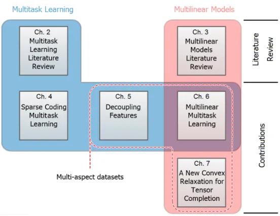
Figure 1.2.: Structure of this thesis.

In this introduction we have highlighted the two key concepts of this thesis, namely neg-ative transfer and multi-aspect data. In the two following chapters, we explore the state of the art in those areas. In particular in Chapter 2, we review MTL approaches based on optimization, and in Chapter 3, we review multilinear models, as the predominant

(26)

models dealing with multi-aspect data. Following the literature reviews, we describe the contributions of the thesis, introduced in Section 1.2. We address sparse coding mul-titask learning in Chapter 4, decoupling of features in Chapter 5, multilinear mulmul-titask learning in Chapter 6, and rounding off the contributions, we describe the novel convex relaxation for tensor recovery in Chapter 7. Finally, we conclude the thesis with a sum-mary of the achievements, and we propose research opportunities that arise from them. Fig.1.2 summarizes the structure of this thesis.

(27)

2. Multitask Learning Literature

Review

In this chapter we survey the multitask learning literature. This survey has two main purposes. Firstly, we present the state of the art in this field, as this provides the starting point of this thesis. In particular, we study models that vary the assumptions made on the data, and examine how they avoid negative transfer. Secondly, we highlight the absence of multitask learning approaches that can leverage multi-aspect datasets.

2.1. Introduction

Multitask learning (MTL) is a machine learning framework which considers several learning tasks together so that by taking advantage of the commonalities between the tasks, it can achieve a better performance than by solving them separately. Its appli-cation is particularly appropriate whenever there are a large number of related tasks to learn and/or when each task has only a small set of instances from which to learn. MTL is inspired by the fact that human beings are able to improve the learning process of a task if it is simultaneously addressed with other related tasks rather than assimilat-ing it in isolation [21]. The literature in psychology [24, 1] show that, for example, the knowledge acquired by human beings while learning physical tasks facilitates the learning process of new motor skills.

Supervised learning problems are not usually isolated in real life, rather they are related to others. As an example we can consider the task of learning the gastronomical pref-erences of a customer, that is, given a description of a dish, we want to learn a function whose output will determine whether our customer will like that dish or not. This is a typical supervised learning task, however in a real situation we will have more than one customer and we will want to build one function per customer to predict her preferences. One reasonable assumption to make is that those functions share some commonalities, such as for example, a set of deciding ingredients. Therefore, the main objective of

(28)

MTL is to try to discover the commonalities between these functions in order to ob-tain a more accurate model. Through the course of this review, other examples will be introduced to illustrate different kinds of multitask relationships.

MTL was proposed in [19, 33, 34, 187] where neural networks, trees and other su-pervised leaning approaches were adapted to deal with MTL scenarios. The empirical results showed a clear improvement over the single task counterpart. Since then, a wide variety of MTL strategies have been proposed and have found applications in many different fields such as machine vision [162, 201, 223], natural language processing [203, 53], biometrics [193] and traffic flow forecasting [93], to name a few.

MTL has strong connections with other established machine learning frameworks, so that research and applications have benefited collectively in those fields. One of them is transfer learning [157] (also known as learning to learn [110] or inductive transfer [47, 164, 176]), whose aim is to extract knowledge from a set of source tasks to be applied in the learning process of target tasks. Therefore, it can be seen as an asymmetric modification of MTL where there is an explicit distinction between source and target tasks. The similarities between MTL and TL are such that several MTL approaches can directly be employed in a TL setting. A different framework is multivariate response learning [14, 28], also known as multi-output learning, which can be seen as a particular case of MTL when all tasks receive the same input data. This category also includes multi-label classification. MTL can also be seen as an extension of matrix completion (or collaborative filtering) [138, 190]. There, the objective is to predict entries in a matrix where only a small subset of them is known. Matrix completion has received increasing interest lately as a way of evaluating items through the ratings of other users. It can be considered as an MTL problem by treating users as tasks where the input data are indicators of the items and the labels are the actual values of the entries in the matrix (conversely, one can consider items to be tasks and input data to be indicators of the users).

In this literature review, we focus on MTL approaches based on regularization on the task parameters to encode the relationships assumed among the tasks. There are three important categories of MTL approaches which can be distinguished by the assumptions encoded in the regularizer:

• Modelling the proximity of the parameters of all tasks by making use of quadratic norms.

• Modelling structure sparsity by employing extensions of the Lasso.

(29)

2.2 Notation

spectral norms.

As we will see, many MTL approaches are based on one of these frameworks, or build upon them introducing further constraints which incorporate more complex or more rich relationships among all tasks. Nevertheless, there are other methods that do not fall within any of those categories, they will also be briefly reviewed.

We introduce the notation which will allow us to formally define the three frameworks and study them. We then review extensions of these frameworks which consider more complex relations among tasks. Next, we address those approaches which fall outside the previous categories. Finally we conclude with a discussion of the approaches.

2.2. Notation

In the following we focus on regression problems but the generalization to classification problems is usually straightforward. In most cases we assume the following setting: the model we want to build has to be able to learn a set ofT linear tasksft(x) = hwt, xi,

x, wt∈Rd,∀t ∈[T], wheredis the dimensionality of the data, and[N]denotes the set

of natural numbers from1toN. In order to learn these tasks, a set of labeled instances is provided: {Xt, yt}, Xt ∈ _Rd×mt_, _yt _∈

Rmt, where Xt is the matrix composed

of all the mt instances provided for task t as columns and yt is the vector containing

the labels. With a slight abuse of notation, we denote X = nX1, X2, . . . , XTo and

Y = ny1_{, y}2_{, . . . , y}To_{. Let} _W _{be the matrix composed of the}_T _{weight vectors}_w tas

columns, that is,W = [w1, . . . , wT]. When making reference to thei-th element ofwt

we use the notationwi,t.

The notation k·k makes reference to norms of vectors or matrices. In the case of ma-trices we will consider the Frobenius norm,k·k_Fr, as well as other norms which will be introduced as they are needed.

We will denote as 1 the column vector whose all elements are 1. Its dimensionality should be clear from its context. The trace of a square matrixAis denoted astrace (A)

and its determinant as det (A). Given any matrix B ∈ _Rd1×d2_{, its singular values are}

represented as σ(B) = (σ1(B), σ2(B), . . . , σK(B)), where K = min{d1, d2}and

σ1(B) ≥ . . . ≥ σK(B) ≥ 0. We denote by |B| ∈ Rd1×d2 as the matrix composed of

(30)

the columns ofB, that isvec (B) =         B1 B2 .. . Bd2         .

2.3. MTL Regularizers

In this section we will consider MTL approaches which share the following optimization problem skeleton: min W R(W), R(W) = T P t=1 X t>_w t−yt 2 2+γΩ (W),

where Ω : _Rd×T → _R+, called the regularizer, provides an intuitive mechanism to

incorporate similarities among tasks weight vectors; and γ > 0 is a hyperparameter which needs to be tuned (for example by cross validation on the data) and regulates the importance of the regularizer with respect to the empirical loss. As noted in the intro-duction, we will consider three kinds of functionsΩ, which implement three different assumptions on the structure of the relationships between the tasks. These functions are:

• Quadratic norms

Ω (W) = vec (W)>Evec (W), (2.1)

whereE ∈_RdT×dT_,_E ₀_.

• Sparsity inducing norms

Ω (W) =ω(|W|), (2.2) whereω : _Rd₊×T →_R+. • Spectral functions: Ω (W) =ω(σ(W)), (2.3) whereω : _RK + →R+.

Note that the case of learning all tasks independently by employing a square norm as a regularizer on the parameters is a particular instance of all three frameworks.

(31)

2.3 MTL Regularizers

2.3.1. Quadratic norms

One way of defining relations among a set of tasks is by looking at similarities between their parameters. For example, let us consider the problem of detecting different fruits in pictures. We want to learn one task function per fruit, e.g. forange(x) will return1

if there is an orange somewhere in the picture x, or −1 otherwise. It is reasonable to accept that the process of detecting an orange in a picture is somewhat similar to the process of detecting an apple, as they have similar shapes. Thus, one may then assume that the parameters defining those functions are close to each other; therefore, one could penalize the distances among them. In this section we focus on linear functions and the use of regularizers of the form described in eq. (2.1), which are useful to model this kind of relationship. In the general case, the objective function to be minimized can be expressed as: R(W) := T X t=1 X t> wt−yt 2 2 +γvec (W) > Evec (W), (2.4)

whereE is defined a priori so that it captures the relations between the tasks. SinceE is positive semidefinite, problem (2.4) is convex.

We study two alternative perspectives of problem (2.1): the feature space and the mul-titask kernel point of view. After that we will review some instances of this framework from the literature.

2.3.1.1. Feature space viewpoint

Let us start by assuming that all functionsftcan be written in terms of the same feature

vectorθ ∈_Rp_{, for some}_p_∈

N,p≥dT, that is:

ft(x) =θ>Btx, x∈Rd,∀t∈[T], (2.5)

or equivalently wt = Bt>θ, where Bt are prescribed p ×d matrices which are task

specific, whereas the vectorθis common to all tasks. Then, we can consider the regu-larization problem characterized by the following objective function:

S(θ) := T X t=1 X t> B_t>θ−yt 2 2+γθ > θ (2.6)

(32)

fea-ture matrixB ∈_Rp×dT _{formed by concatenating all}_B

tmatrices:B := [Bt : ∀t∈[T]].

The equivalence between these two problems relates matrixB to matrixE in eq. (2.4). Specifically, [58, Prop. 1] establishes that:

If the feature matrixB is full rank and we define the matrixE in eq. (2.4) to beE =B>B−1, then we have that

S(θ) =RB>θ, θ ∈_Rp_. _(2.7)

Conversely, ifE is a symmetric and positive definite matrix,T is a squared root ofEand we setB =T>E−1_{, then eq. (2.7) holds true. Moreover, the}

unique minimizersW∗of problem (2.4) andθ∗of problem (2.6) are related by the equationvec (W∗) =B>θ∗.

The above proposition requires matrixE to be positive definite and the matrixB to be full rank. Note that otherwise the functionsftare linearly related. We can see as a trivial

example the case that Bt = B0, ∀t ∈ [T], for some prescribed matrix B0 ∈ Rp×d. In

that case all tasks are the same task,f1 =f2 =. . .= fT, so effectively we are solving

a single task learning problem on all theT mdata instances from theT tasks.

When the matrix B is not full rank, the equivalence in eq. (2.7) between functions (2.4) and (2.6) still holds true provided that matrixE is given by the pseudoinverse of matrixB>B and we minimize function (2.4) on the linear subspace S spanned by the eigenvectors of E which have a positive eigenvalue. For example, in the above case whereBt= B0,∀t ∈ [T], we have thatS ={(wt : t ∈[T]) : w1 =w2 =· · ·=wT}.

This observation would also extend to the circumstance where there are arbitrary linear relations amongst the tasks.

2.3.1.2. Multitask kernel viewpoint

In this section we study another viewpoint of quadratic norms based on the use of a kernel (see [179] for a review on kernel methods). Making use of the previous viewpoint where eq. (2.4) can be expressed as a single task learning problem, we can consider a kernel defined on a multitask setting. We can start by considering the functions f = (ft : t ∈[T])as the real-valued functions(x, t)7→θ>Btxon the input spaceRd×[T]

whose squared norm isθ>θ. The corresponding reproducing kernel is:

(33)

Since eq. (2.6) is like a single task regularization functional, by making use of the representer theorem its minimizer can be expressed as:

θ∗ = P

i∈[m] P

t∈[T]

citBtxti.

Consequently, the optimal task functions can be expressed as: f_q∗(x) = P

i∈[m] P

t∈[T]

citK((xti, t),(x, q)), x∈Rd, q∈[T],

2.3.1.3. MTL models based on quadratic norms

Here we present two very common MTL approaches which exploit quadratic norms to model the proximity between tasks. In the following examples, we consider a special subset of quadratic regularizers of the form:

Ω (W) = X

t,s∈[T]

w_t>wsGts, (2.9)

whereGis a prescribed positive definite matrix. Matrices Gin eq. (2.9) andE in eq. (2.4) are related by the equalityE =G⊗Id, where⊗denotes the Kronecker product

[119].

Penalizing task’s variance

Let us assume that all tasks weight vectors are close to a reference vectorw0which also

needs to be learned. This idea was proposed in [59], where the authors assumed that wt=w0+vt,∀t∈[T],

where vt is what makes task t different from the others and therefore it is assumed to

be small. This assumption is taken into account by adding regularization terms which penalize the square distance between anywtandw0 (in other words, penalizingkvtk

2 2,

∀t∈[T]). The resultant approach is based on the following regularizer:

Ω (W) = min w0 1 λT T X t=1 kwt−w0k22+ 1 1−λkw0k 2 2, (2.10)

where λ ∈ [0,1] is a regularization parameter which needs to be tuned a priori. It controls the prior information we have about both how closew0 is to0, and how close

(34)

all weight vectorswt are tow0. The first condition is encouraged for high values of λ

whereas the second condition becomes more important for values ofλclose to0. This regularizer can be expressed directly in terms ofW getting rid ofw0in the

follow-ing manner [58]: Ω (W) = 1 T   T X t=1 kwtk2₂+ 1−λ λ T X t=1 wt− 1 T T X s=1 ws 2 2  . (2.11)

From this point, it can be worked out thatG = _T1 _λ1IT − 1_{T λ}−λ11>

. By applying the results in eq. (2.7) we obtain thatB is characterized in the following way:

Bt= [ √ 1−λId,0d, . . . ,0d | {z } t−1 ,√λT Id,0d, . . . ,0d | {z } T−t ] (2.12)

where0d ∈ Rd×d denotes the all zeros matrix. Finally we derive the multitask kernel

associated to regularizer in eq. (2.10). Applying eq. (2.8) we have that: K((x, t),(z, s)) = (1−λ+λT δts)x>z, x, z∈Rd, t, s ∈[T].

Note that this set of kernels defined in terms of λ ∈ [0,1] is a convex hull of two kernels. One of them (whenλ = 0) treats all tasks as the same task whereas the other (whenλ= 1) tackles all tasks independently.

Hierarchical Regularization

Let us now assume that the tasks are organized according to a prescribed hierarchical structure or tree which contains information about how tasks are related, in the sense that each task weight vector is close to the task weights of their children. A motivating example is object recognition on classes that are organized in a hierarchy. In this way, the leaves represent elementary classes and are associated to superclasses (for example, leaf nodes could correspond to classes such as “cars”, “vans”, “bikes” and could all be children of the super-class “vehicles”). Following the idea of the previous method, we assume that the tasks are close to each other according to the prescribed hierarchical structure. Therefore, we want to set out the following regularizer [58, 201]:

Ω (W) = T X t=1 kwtk 2 2+ 1−λ λ T X t=1 wt− 1 |Ct| X s∈Ct ws 2 , (2.13)

(35)

where Ct represents the set of children of task t, and |Ct| is its cardinality. Let us

introduce the operatorparent : [T] → {[T],0}, which returns the parent of the input according to the given tree. If the input task is the root, the output is0. We consider the symmetric matricesS, P ∈_RT×T _where_S_{indicates sibling relationships among tasks:}

Sts =        1 |Cparent(t)| 2 if parent (t) = parent (s) 0 otherwise ,

andP encodes parent-child relationships:

Pts =            1 |Ct| ift= parent (s) 1 |Cs| ifs= parent (t) 0 otherwise .

Then, the matrixGcorresponding to the regularizer in eq. (2.13) can be expressed as: G= _T1 1_λIT +1₂−_λλS− 1−_λλP

.

The characteristic matrixB and the induced kernel can be calculated from this form of G.

2.3.1.4. Discussion

The MTL approaches that arise within this framework are based on the similarity be-tween the weight vectors of the tasks. This intuitive assumption is useful to model the relationship of tasks that are positively correlated. However, the simplicity of quadratic norm methods makes them unable to capture more complex relationships. One simple example when these approaches fail is when two tasks produce uncorrelated outputs to the same inputs. Utilizing quadratic norms in such situations would lead to nega-tive transfer. In the following sections we review approaches capable of leveraging this and other more general relationships, and which can positively transfer the knowledge between tasks.

2.3.2. Sparsity inducing functions

The approaches described in this section assume sparse structure in the task’s weight vectors. This is very useful in situations where the dimensionality of the data is large.

(36)

For example, let us think about the problem of discovering how different DNA microar-rays, which are high dimensional entities, lead to a related set of cancers. One can model this problem by considering one task per cancer type. An assumption made in address-ing this problem is to postulate that these kinds of cancer are related because they are caused by the same sets of genes in a microarray [98]. In other words, all tasks depend only on a small subset of the attributes which describe the input data. Sparse solutions are encouraged by the regularization functions explained in this subsection. These reg-ularizers build up on the Lasso technique [196], which encourages sparsity on a weight vector elements by penalizing its`1-norm. The method of`1-norm regularization has

proven to be superior to non-sparse methods such as`2-norm regularization whenever

there is a priori knowledge about the sparsity of the explanatory variables [145].

Sparse methods are also useful when the objective of the model is not only to be accurate but also to be highly interpretable. Interpretable solutions are very important in many fields such as medicine [98]. In this case, even with a lack of prior knowledge, one can sacrifice some accuracy of the model in order to get a solution which is a function of a small set of explanatory variables.

2.3.2.1. `p,1-norms

Some MTL approaches extend the Lasso by assuming that all tasks use the same sparse set of attributes.

One of the first works that formulated this hypothesis and proposed a solution is [204]. Its authors propose to shrink the`1-norm of the maximum absolute value of each

ex-planatory variable weight across all tasks. In other words, they propose the use of the `∞,1-norm, kWk_∞_,₁ = Pd i=1 T max t=1 |wi,t|.

The authors justify this choice by arguing that the quantity maxT

t=1 |wi,t| can be seen as

the “simultaneous explanatory power” of variableiamong all tasks. Furthermore, this regularizer is appealing since it keeps the objective function convex. In order to solve the resultant problem, the authors employ an interior-point algorithm. This approach, which is also known as Multitask Lasso [116], is theoretically studied in [143], where the authors provide some results which establish conditions under which employing the `∞,1-norm is advantageous over the use of the `1,1-norm,kWk₁_,₁ =

T P t=1 d P i=1 |wi,t|, that is

(37)

the`1-norm of the matrix elements. Note that the latter regularizer does not provide any

shared sparsity between tasks.

Another approach is the adaptation of Group Lasso [222] to MTL. Group Lasso is a sin-gle task supervised learning method which assumes that all attributes can be organized in several disjoint groups so that some groups of attributes are important for the solution whereas some others can be ignored. These groups of attributes are known a priori so the problem consists in minimizing a loss function plus some regularizer which induces sparsity over groups but not within groups.

This strategy can be directly applied to an MTL setting by assigning each of these groups to the same attribute employed by the different tasks. This implies the use of the `2,1

-norm onW, which is defined askWk₂_,₁ = Pd

i=1 T P t=1 w2 i,t !1 2

. This idea is proposed in [8, 150, 151] and is known as multitask joint covariate selection [151]. The corresponding optimization problem is then

argmin W T X t=1 X > t wt−Yt 2 2+γkWk2,1. (2.14)

Let us recall that matrixWcontains the weight tasks vectors in columns so the`2,1-norm

encourages that matrix to have a few non-zero rows, or attributes weights.

As we can see, the last approaches are very similar and are all instances of the`p,1-norm,

defined as: kWk_p,₁ = Pd i=1 T P t=1 w p i,t !1_p .

As stated by [218], the`∞,1regularizer encourages all non-zero parameters to have the

same absolute value across all tasks, whereas when employing the`2,1 regularizer, the

resultant non-zero values of the parameters across tasks have usually a higher variance. Indeed we can make the generalization to any`p,1-norm forp >1(note thatp= 1leads

to the original Lasso technique implying that all tasks are assumed to be independent). Further development based on the Group-Lasso approach has been done in several works, and different optimization strategies have been suggested to solve problem (2.14). In [117], the authors propose an optimization approach based on proximal methods [144] whereas in [8] the authors develop an alternating algorithm which minimizes an objective function whose regularizer is the square norm of the `2,1-norm of W. In

[150, 151] the authors also propose a method to efficiently compute the space of so-lutions provided by the algorithm for all values ofγ (regularization path). In [41], the

(38)

authors consider the case when different attributes have different regularization param-eters (values), develop a method to automatically tune them and provide some theoreti-cal statistitheoreti-cal guarantees on its performance. Finally, in [120] the authors provide some learning bounds on this framework, which show that there are theoretical advantages of this approach over performing the Lasso on all tasks independently.

2.3.2.2. Other sparsity inducing functions

Even though assuming that all tasks use the same subset of attributes is the most com-mon conjecture acom-mong sparsity MTL methods, there are other scenarios where different sparsity patterns could be useful.

Exclusive Lasso In [227], the authors propose a different scenario: they assume that tasks tend to not share any attributes between them. This can be useful, for example, in multi-category document classification, where different categories of documents are characterized by different words (attributes). In order to model this, they propose the following regularizer: Ω (W) = Pd i=1 T P t=1 |wi,t| !2 .

Note that the inner sum is the`1-norm of the tasks values for the same attribute and thus

encourages sparsity (or heterogeneity) of attributes across the tasks. The outer sum, which is the`2 norm of the previous values, combines the weights of all attributes.

Tree-Guided Group Lasso Let us now consider the scenario where the model is provided with extra information about the tasks (as considered in Section 2.3.1.3), where this is given as a hierarchy of tasks indicating relationships among them. In [99] the authors consider this situation in the context of sparsity parameters. Their key assumption is that any common ancestor of two leaves of the tree (tasks), contains information about the attributes which are used simultaneously by both tasks. This is induced by building a regularizer composed of a weighted sum of`2,1-norms on the tasks

weight vectors according to the hierarchy. Particularly, the authors place an `2,1-norm

regularizer on each node of the hierarchy. This term is multiplied by a weight which is determined by parameters sv and gv, where sv +gv = 1. The vector gv represents

the joint selection of the attributes for tasks under node v, whereas sv represents the

(39)

The authors prove that the total weight related to any task weight vector is 1, which provides the framework with consistent estimators. Since knowing a priori the hierarchy among tasks (as well as the values ofsv andgv for all nodes in the tree) can be a strong

assumption in many real cases, the authors suggest the previous use of methods such as hierarchical agglomerative clustering algorithm to estimate the underlying structure.

2.3.2.3. Discussion

In this section we have described a set of MTL methods based on imposing sparsity patterns to the task’s weight vectors. Hence, the set of attributes of the data which are meaningful for the tasks can be filtered from the remaining ones. These approaches are useful whenever the dimensionality of the data is high and only a few attributes of the data convey meaningful information. However in several situations this does not hold. For example when the input data are images usually the majority of pixels provide useful information. In that case it is reasonable to look for higher level features that can be meaningful for all tasks. This more general approach is taken in the following section. It is also worth remarking that the ideas used in Exclusive Lasso, which imposes heterogeneity between the attributes used in tasks, could potentially be useful for multi-aspect datasets, because different multi-aspects of data may depend on different features.

2.3.3. Spectral functions

In this section, we consider a different kind of relation to link tasks together: all tasks share a low dimensional representation of the data. In other words, we assume that the task’s vectorswtare linear combinations of a few common basis vectors which need to

be estimated from the data. Another viewpoint can be explored by comparing this set of approaches and the unsupervised approach of principal component analysis (PCA) [160]. The latter procedure obtains a set of components (linear combinations of the attributes) so that when projecting the original data onto them, the resultant projections have the largest possible variance. In contrast, in MTL spectral function approaches, the components are extracted so that they are as useful as possible for all tasks.

Let us imagine an automatic system whose purpose is to infer levels of different affective states (such as anger, boredom and happiness) in images of faces. The MTL model may consider one task per affective state. It seems reasonable to assume that there exists a small set of components of faces which are enough to discriminate any kind of information regarding affective states. Note that, unlike the previous strategy, the

(40)

features used now do not necessarily correspond to a particular part of the face (e.g: eyes, ears or noses), but to linear configurations of the whole face, which are learned in the process.

One way to encourage the above assumption is by using certain spectral regularizers. Let us recall that a spectral function of a matrix M ∈ _Rd1×d2_, _ω₍_M₎ _{is any function}

that only uses the singular values ofM, σ(M)∈_RK_{, where}_K _{= min}_{_d

1, d2}. These

functions are especially useful since the singular values of a matrix convey determinant information regarding its structure.

2.3.3.1. Rank

Let us continue with the previous affect recognition example from faces. In that scenario we have a set of faces composed ofdpixels (attributes) and the objective is to learnT affective recognition tasks. The assumption that one may impose is that all tasks use a common set of K linear features from the data, whereK d. Therefore, one can model it by settingft(x) =wt>x=a

>

t B

>_{x, where}_B _∈

Rd×K is the matrix composed

of K learned linear projections common across the tasks, and at ∈ RK specifies the

way these projections are linearly combined to obtain the weight vector for taskt, wt.

Then we would like to solve the following non-convex problem:

min A,B T X t=1 X t> Bat−yt 2 2, (2.15)

where matrixA = [a1, a2, . . . aT]. Matrix B can be seen as the factor which limits the

input data information the tasks have access to. Therefore, by learning theK features which compose B, the model may improve the performance on all tasks. Note that solutions to problem (2.15) are not unique: if we consider any nonsingular matrixC ∈

RK×K, then W = BA = (BC) (C−1A). An equivalent problem can be obtained by

expressing the objective function directly in terms of the tasks weight vectors:

min W T P t=1 X t>_w t−yt 2 2 s.t : rank (W)≤K or equivalently min W T X t=1 X t> wt−yt 2 2 +γrank (W) (2.16)

for some value ofγ, making clear that the resultant problem is a spectral regularization problem.

(41)

optimization problems, where finding the optimal solution is intractable for the gen-eral case. However, we can obtain this optimal solution if we consider a multivari-ate response problem, that is, when all tasks share the same input data X1 ₌ _X2 ₌

· · · = XT = X. Let us assume that ΣXX ∈ Rd×d is the input covariance matrix and

ΣY X ∈ RT×dis the cross covariance matrix between the outputs and the inputs. Then

the optimal solution to problem (2.16) can be expressed as [14]: W∗ = PK

k=1

VkVk>ΣY XΣ−XX1 ,

whereVkis thek-th singular vector ofΣY XΣ−XX1 Σ

>

Y X.

In the general MTL setting, problem (2.16) is quite demanding since the regularizer is neither convex nor differentiable, and in addition the resultant problem is NP-hard [11]. In the following we will cover some more feasible approximations.

2.3.3.2. Trace norm

Let us continue from eq. (2.16), where the rank ofWacts as the regularization function. In order to make the problem tractable we can look for an approximation of the rank function which keeps the whole problem convex. A good candidate function for that is the trace norm, which is defined as the sum of the singular values of the matrix. It has the interesting property to be the convex envelope of the rank in the spectral ball [61]. The trace norm as a regularizer was first proposed in [61] and since then it has been employed in many problems involving the rank of a matrix to be learned [8, 166, 165, 32, 190, 191]. In our case, the resultant problem is

min W T X t=1 X t> wt−yt 2 2+γkWkTr. (2.17)

In the following, we consider two alternative viewpoints of this objective function.

Square Frobenius norm viewpoint A way to interpret eq. (2.17) is by means of the approach suggested by [4]. In this paper the authors propose a method which explicitly learns a common representation of the input data which is used for all tasks. Particularly, they propose to express each task weight vector aswt =Bat, in a similar

way as in eq. (2.15). In order to avoid overfitting, the authors add the square Frobenius norm onA(the matrix composed of all at, ∀t ∈ [T]as columns) andB. The resultant

(42)

optimization problem is min A,B T X t=1 X t> Bat−yt 2 2+ γ 2 kAk2_Fr+kBk2_Fr. (2.18) This problem is not convex and the numberK of factors, or linear projections, needs to be defined a priori. In order to account for both issues, the authors use the following equivalence [190]: kWk_Tr= min BA=W 1 2 kAk2_Fr+kBk2_Fr

in eq. (2.18) leading again to eq. (2.17). It is important to remark that problem (2.18) is equivalent to problem (2.17) only whenK ≥ min (d, T). Notice that if this is not the case, we are adding a rank constraint onW to be less or equal thanK, leading to a non-convex problem.

`2,1-norm viewpoint Another interpretation can be found by considering the

prob-lem proposed in [8]: min U,A ( _T X t=1 X t> U at−yt 2 2+γkAk 2 2,1 : A∈R d×T , U ∈_Rd×d, U>U =I ) (2.19) In this approach the matrixU is used to rotate the data, so that there are some projections which can be useful for all tasks. Consequently,U is constrained to be an orthonormal matrix. The matrixAcontains, for each columnt, the weights of tasktfor the compo-nents learned inU. Since the original assumption was that all tasks use the same low dimensional representation of the data, an`2,1-norm based regularization term is added

so thatAis encouraged to have only a few non-zero rows. The productU atmakes the

problem (2.19) non convex, however the authors of [8] show that this is equivalent to the convex problem:

min W,D T P t=1 X t>_w t−yt 2 2+γ T P t=1 w_t>D−1_w t s.t : W ∈_Rd×T_{, D} _∈ Rd×d, D 0,tr (D)≤1, (2.20)

where W = U A. Finally, solving this problem with respect to D and plugging it back into problem (2.20) leads to a similar formulation as in eq. (2.17) but where the regularizer takes the form of the square of the trace norm. This set of equivalences is to be expected since minimizing the rank ofW =U A, withU orthogonal, is equivalent to minimizing the number of n