Predicting User Interaction on Social Media using Machine Learning

(1)

DigitalCommons@UNO

Student Work

11-2018

Predicting User Interaction on Social Media using

Machine Learning

Chad Crowe

University of Nebraska at Omaha

Follow this and additional works at:

https://digitalcommons.unomaha.edu/studentwork

Part of the

Computer Sciences Commons

This Thesis is brought to you for free and open access by

DigitalCommons@UNO. It has been accepted for inclusion in Student Work by an authorized administrator of DigitalCommons@UNO. For more information, please [email protected].

Recommended Citation

Crowe, Chad, "Predicting User Interaction on Social Media using Machine Learning" (2018).Student Work. 2920.

(2)

Media using Machine Learning

A Thesis

Presented to the

College of Information Science and Technology and the

Faculty of the Graduate College

Universityof Nebraska at Omaha

In Partial Fulfillment of the Requirements for the Degree Master of Science in Computer Science

by Chad Crowe November 2018 Supervisory Committee Dr. Brian Ricks Dr. Margeret Hall Dr. Yuliya Lierler

(3)

ProQuest Number:

INFORMATION TO ALL USERS

The quality of this reproduction is dependent upon the quality of the copy submitted.

In the unlikely event that the author did not send a complete manuscript

and there are missing pages, these will be noted. Also, if material had to be removed, a note will indicate the deletion.

ProQuest

Published by ProQuest LLC ( ). Copyright of the Dissertation is held by the Author.

This work is protected against unauthorized copying under Title 17, United States Code Microform Edition © ProQuest LLC.

ProQuest LLC.

789 East Eisenhower Parkway P.O. Box 1346

Ann Arbor, MI 48106 - 1346

10974767 10974767

(4)

Predicting User Interaction on Social Media using Machine Learning Chad Crowe, MS

University of Nebraska,2018 Advisor: Dr. Margeret Hall

Analysis of Facebook posts provides helpful information for users on social media. Cur-rent papers about user engagement on social media explore methods for predicting user engagement. These analyses of Facebook posts have included text and image analysis. Yet, the studies have not incorporate both text and image data. This research explores the usefulness of incorporating image and text data to predict user engagement. The study incorporates five types of machine learning models: text-based Neural Networks (NN), image-based Convolutional Neural Networks (CNN), Word2Vec, decision trees, and a com-bination of text-based NN and image-based CNN. The models are unique in their use of the data. The research collects 350k Facebook posts. The models learn and test on advertise-ment posts in order to predict user engageadvertise-ment. User engageadvertise-ments includes share count, comment count, and comment sentiment. The study found that combining image and text data produced the best models. The research further demonstrates that combined models outperform random models.

(5)

Chapter 1

Introduction

The majority of Americans engage on social media (Smith 2018). This is due in part to social media’s low barriers (Azizian et al., 2017). For example, anyone can scroll through a Twitter or Facebook feed. Yet, there is another side of social media. Not all users on social media consume content. Social media platforms provide interfaces for advertisers. On these platforms, companies pay a small fee to display their ads. Social media is having a larger influence on businesses and consumers (Fisher 2009). This creates a massive conglomerate of marketing. Each of these companies wants to reach customers with their products. They trust that social media is an effective means to reach target audiences. Often, social media platforms let companies specify advertisement demographics. Targeting information ensures that advertising money is well spent. Investors spend billions of dollars to advertise on social media (Statista 2018). These investors care about the efficacy of their social media spending.

This creates a large challenge for social media platforms. Social media platforms need to provide the ability to connect companies with users. The field of advertising on social media is new. Platforms want to justify their effectiveness to potential advertisers. Measuring

(8)

this effectiveness after advertising is possible. Yet, companies prefer a way to calculate return on investment (ROI) before investing. One way to calculate ROI is to measure user engagement. This study predicts user engagement for advertisement posts. The user engagement metrics include share count, comment count, and comment sentiment. This study explores predicting user engagement with different types of machine learning models. The models are unique in their incorporation of text and image data. The goal is to understand which model-types best predict user engagement.

The research applies these models to a real-world use-case. The research uses models, which can predict user engagement, in order to vet for better performing ads. Platforms could use these models to inform advertisers which of their ads will perform best on the platform. This allows advertisers have their ads vetted. The vetting could prevent adver-tisers from spending a lot of money showing worse ads. Moreover, the vetting would allow advertisers to only show ads that will perform best.

1.0.1 Problem

Almost 70% of adults use Facebook (Gramlich 2018). Running such a large site for many users is expensive. Yet, users pay no fee for using Facebook. Google is like Facebook in that it also provides free services to users. The services are free because platforms generate revenue from advertising. Google generates more than 70% of its revenue from advertising (Statista 2017). Facebook generates more than 80% of its revenue from advertising (Statista 2018). Advertising is not without difficulties. Most people do not like advertisements (Shi, X. 2017). In fact, people generally feel annoyed by advertisements (Shi, X. 2017). Users will even avoid advertisements (Shi, X. 2017). This results in users using social media less. Fewer users mean that advertisements receive less engagement. Lower user engagement means the

(9)

platform makes less money. Fewer users also mean that platforms are unable to reach as many people. In this way, advertisements can hurt the platform and advertisers. The challenge is to deliver relevant content to users. The content might agree with user interests, hobbies, and preferences. If advertisers can deliver relevant content, then advertisers, users, and the platform benefit. The users buy content. The advertiser’s sell merchandise and the platform make money. Yet, there are millions of users on social media and many advertisements (Smith 2018). This thesis aims to explore this problem by predicting user engagement. This helps companies better understand how their advertisement will perform on social media. It also gives advertisers feedback. More confident advertisers will invest more on the platform.

The thesis performs its analysis on the Facebook post with image and text data from a Facebook post as input. The research performs computations on the data and predicts user interaction. The aim of the thesis is to predict user interaction. The thesis will explore this prediction with different machine learning models. The analysis used the Facebook post since it contains image and text data. Its data is also available via Facebook’s Graph API. The study collected and trained on exactly 350k posts. The Facebook post is generic. Other platforms have similar representations of the Facebook post. These include tweets and Pinterest posts. The posts in this study are from advertisers. This limitation might simplify the models.

Previous studies have modeled user interaction on social media (Straton 2015). The paper refers to post metrics as post-performance. Facebook refers to the metrics as user interactions, or engagements (Facebook API). The Facebook post may include text, an image, and meta-data. The meta-data includes shares, comments, and data from the post’s Facebook page. The metrics denoting user interaction include the number of shares and the

(10)

comments. The scope of the research will consist of predicting these metrics. The research creates many types of machine learning models. The research will uncover which can best predict user interaction. One goal is to model user interaction with both text and image data. The study will gauge how well models can predict user interaction.

1.0.2 Thesis Structure

The rest of Chapter 1 will explain the motivation for the research. Chapter 2 will explore the related work. Chapter 3 will address the research gaps and define the research questions. Chapter 4 will present the research methodology. Chapter 5 will explain machine learning model methodology and data processing. Chapter 6 will present the results and chapter 7 will discuss the results. Finally, chapter 8 will present the study’s conclusions.

1.1

Scope of Study

The study explores three types of models. These are text-based, image-based, and those that combine text and image data. The scope of the study limits both its input and output data. Its input data includes the post’s text and an image if present. The output is user interaction. The user interactions considered include share count, comment count, and comment sentiment. These outputs were the available user interactions from the Facebook API. These inputs are ubiquitous on Facebook and common on other social media platforms. There was enough Facebook data to train all but one type of the machine learning models. Even more, each post always has some share count, comment count, and comment sentiment. The study has interest in the benefits and effects of combining image and text data. The study will also determine if the model is useful in practice. The study will compare the model’s performance with a random model.

(11)

1.2

Scenario

This thesis will be dealing with social media data. Specifically, Facebook posts and its associated data. This thesis will use this data to build machine learning models. These models will predict post data. This research is most interested in what features improve predicting aspects of user interaction. This study defines user interaction number of shares, comment count, and the sentiment of those comments. This paper hopes to use these metrics to generate predictive models.

The techniques will include data transformation, post-analysis, and the creation of machine learning and statistical models to fit the data. The goal is to create a generative predictive model for any social media post. The problem under consideration is one of regression. An overarching goal of the thesis is to predict user interaction. Given a Facebook post and its contextual information, predict the number of shares and comments received by that post. This contextual information includes the post’s accompanying text and photo.

1.3

Significance of Study

The study contributes to understanding user engagement on social media. The study also highlights which models best predict user interaction. The research will uncover how well models can measure user interaction. The paper will also discuss how models can predict with both image and text data. On a practical level, the models could be a tool for platforms and help advertisers. The study also serves as an overview for approaching user interaction prediction.

(12)

1.4

Motivation

There exist a great number of algorithms which interact with social media. Kaggle hosted a competition for the company Avazu for predicting click-through rate using ad data (Kaggle 2015). Yet, a download of their dataset showed that the provided input variables focus on where the ad was displayed, where the ad was hosted, the type of ad that was displayed, and the device the ad was viewed on. While these can provide a great deal of explanation, they lack the most important information, i.e. the ad itself. Other studies predicting click-through rates have focused on the text content of the ad (Li et al., 2015). Yet, these studies oversimplify the data. The vast majority of advertisements on social media consist of text and image data. When users interact with ads, they are mainly interacting with the content of the ad. It seems like the best way to approach predicting user interaction must include this ad data. Moreover, it is commonly said that a picture’s worth a thousand words. Any analysis which eclipses this data is likely short-sided and suffer in precision. New analyses should include both text and image data.

It is no surprise that the analysis of images on social media is largely under-addressed. Images are notoriously difficult to analyze. They are wrought with noise, colors, and might contains many objects at many angles. Moreover, images might contain text and often convey meaning. This represents a massive amount of variance in image data. This degree of complication makes images both interesting and notoriously difficult for analysis.

In recent years, more APIs and tools have been created to perform object identification and feature detection on images. Their algorithms perform object identification and identify similarities between images. Many a paper has performed sentiment analysis on images (Wang et al., 2015). The ability to discover similar images, their objects, and its sentiment provides an opportunity for using this data in social media analysis.

(13)

The increase in machine learning libraries includes implementations for image-related algorithms. Convolutional neural networks are more accessible due to libraries like Keras and TensorFlow. These convolutional neural networks give their users the ability to perform better image analysis. They have been most widely used in image classification. They also have applications in image clustering and textual synthesis. These are new tools for researchers within the domain of image-analysis. They provide the ability to improve upon current social media analysis by also analyzing image data.

Social media provides an optimal environment for such research. A great deal of its data is publically available through social media platform APIs. Such APIs provide textual and image data at a massive scale. This data can be downloaded, transformed, and organized for large-scale machine learning analysis.

These new tools, techniques, and availability of data provide an exceptional opportunity to improve upon current social media analysis. These also provide opportunities to develop new techniques and discover important features for social media analysis. This paper seeks to append to this largely under-addressed field within academia.

(14)

Chapter 2

Related Work

2.0.1 User Interaction Studies

Li et al. predicts click-through rates on Twitter (2015). Click-through prediction estimates the likelihood for users to click on advertisements. For example, a user might view some merchandise on Amazon. Amazon then stores a cookie in that user’s browser. Later, while on Twitter, Amazon will pay Twitter to reshow this merchandise on the user’s feed. The study itself predicts the likelihood of ad clicks on user feeds. This likelihood is difficult to calculate since clicks are few and far between. The probability of ad clicks is often a fraction of a percent. The goal is to model the likelihood of user clicks. The study made predictions by correlation user interests with ad relevance. The study also modeled twitter sessions for the study.

Stranton et al. predicts user interaction on Facebook with post, text, and time data (2015). The study predicted page likes, shares, and comment counts from this data. The analysis categorized all posts into categories of low, medium, and high engagement. A neural network trained on this data. The study was successful at predicting for low user

(15)

engagement. The neural network performed poorly at predicting higher levels of engage-ment. The particular study sampled from public health data. The study’s sample size was 100k posts. The study did not incorporate images or comment text in their predictions.

Ohsawa and Matsuo investigated predicting user interaction for Facebook pages (2013). The study predicted paged likes based on the page description. The study creates a neural network of pages based on their entities. The page like prediction relies on the number of likes on similar pages. The model used like counts from Wikipedia pages for its prediction. The final model could predict Facebook page likes with a high degree of precision.

Text sentiment on social media is the subject of many studies. Liu performs opinion mining from social media (2012). Opinion mining works with keywords that are sentiment indicators. Existing sentiment lexicons are available for predicting sentence sentiment. Wang et al. focus on image sentiment analysis by clustering images by sentiment (2015). An unsupervised model trains on the clustered images. Image sentiment is also classified using sentiment banks. An existing model classifies object images. A sentiment bank uses the set of image objects to classify the image’s sentiment.

2.0.2 ROI Studies

Fisher cites that ROI is the Holy Grail of social media (2009). Social media has a growing effect on consumer behavior (Fisher 2009). The study polled for user behavior. 34% of participants post products about opinions on blogs. 36% of participants better rate com-panies with blogs. Moreover, traffic to blogs increased 50% that year, compared to 17% at CNN, MSNBC, and the New York Times. 70% of consumers visit social media sites for information. 49% of the 70% buy based on social media content. 60% of users pass along social media data to other users.

(16)

ROI is difficult to track (Schacht, Hall, Chorley 2015). Most companies are unable to get revenue or cost savings from social media (Romero 2011). Romero calculates ROI for non-profits using the increase in service-use. Romero calculates service use differences between new and old users. However, Romero provides no ROI numbers. Schacht also measures ROI by user consumption. The study performed a cross-platform analysis of ROI on Facebook, Twitter, and Foursquare. Schacht proved that tweets can predict rising Foursquare check-ins.

Tiago polls which social media metrics marketing managers care about most (2014). The results are percentages of marketing managers who consider the metrics important. The most important metrics are brand awareness (89%), word-of-mouth buzz (88%), customer satisfaction (87%), user-generated content (80%), and web analytics (80%). Managers prefer metrics that promote engagement. Such metrics include page views, cost per thousand impressions and click-through rate. 18% of the surveyed companies plan to increase their investments in social media.

2.0.3 Other Research

Image analysis often includes denoising techniques. Using denoising creates an image that is easier to analyze. One such techinque is principal component analysis (PCA). PCA is especially helpful for image denoising. It works on image gradients. An image gradient is the change in pixel intensity from pixel to pixel. A change from black to white represents a large pixel gradient. Such a large gradient generally represents some kind of image edge. An image comprises many pixel gradients in many directions. PCA eliminates pixel gradient directions that contain smaller gradients. The result is an image that preserves strong contrast areas and edges.

(17)

Another important aspect of image denoising is simplifying colors. Colors are often simplified into a single pixel intensity. The final result is a single grayscale pixel intensity. This pixel intensity is the mean weight of the red, green, and blue channels (Kanan and Cottrell, 2012). Kanan and Cottrell explore other methods for calculating grayscale inten-sity. Kanan and Cottrell explore if other grayscale intensity calculations produce better image descriptors. The study used machine learning model performance to measure the grayscale method’s performance. Kanan and Cottrell thought that the mean color intensity might misrepresent features. Kanan and Cottrell point to examples where color-blindness hide image details. By simplifying colors, the final image might lose important information. The study applies feature detection to images. The study ranks the quality of the produced image descriptors. The authors found that methods based on human brightness perception performed worse. Methods that incorporated a form of gamma correction performed best. One such gamma correction algorithm is the Gleam algorithm. This algorithm averages each color after applying a gamma transformation to each channel.

Lowe discusses how to create and collect distinctive image keypoints (2004). The paper presents the Scale Invariant Feature Transform approach (SIFT). The goal is to identify important image keypoints and describe these keypoints. The SIFT algorithm is special because it is invariant to size or rotation. The SIFT algorithm recognizes important keypoints. The algorithm detects these keypoints with image gradients. The algorithm determines keypoint direction of reference by its greatest gradient direction. The keypoint descriptor describes the gradients around the keypoint. The final keypoint descriptors are distinctive. Algorithms can match them to other images. Matching keypoints have a high probability of containing similar objects.

(18)

corner-detection. The algorithms detect image corners with image gradients. The algorithm uses image contours and boundaries to identify corners. The algorithm applies Gaussian blurring to identify corners. The Gaussian blurring emphasizes edges by eliminating noise. The algorithm applies the second derivative to identify curves. The algorithm selects gra-dient curves as optimally stable points for keypoints. Matas et al. (2002) have shown that such features are maximally-stable regions.

Digital image correlation (DIC) is a technique for measuring shape, motion, and image deformation (Chu 85). The technique works by comparing and matching grayscale images from different views. The DIC technique employs a correlation criterion. This detects a best match group of pixels at some keypoint. Chu uses DIC in conjunction with SIFT to detect keypoints. Chu employs an algorithm known as iRANSAC. This algorithm detects false-positive matching keypoints from the SIFT algorithm.

Mandhyani et al. looks into techniques for classifying images (2017). Mandhyani et al. uses a bag-of-visual-words representation. The algorithm works by identifying objects in the image. The algorithm identifies objects with feature detection and keypoint clusters. The features map to databases of object features. The algorithm classifies objects by matching feautes to a feature databbase of objects. The algorithm performs classification with these set of objects. Each object, once identified, maps to words. The algorithm uses these bag-of-words to classify the image. The algorithm uses k-means clustering on image vectors. The created models can classify with accuracies from 50-75

This research explored synthetic textures. Synthetic textures are ways to transform images with convolutional neural networks. Algorithms can apply synthetic textures to images to style them. This research wonders if certain synthetic textures would cause advertisements to perform better. Aittala, Aila, and Lehtinen explore the current work on

(19)

synthetic textures (2016). Studies apply synthetic textures to recreate images with modified color and patterns. Texture synthesis uses a base for its transformation. An image descriptor minimizes image differences, which produces the synthetic image. One large disadvantage is that textures must be manually created. They hold promise for transforming images. Yet, they might be too work-intensive for this study.

Generative modeling has shown promising results in texture synthesis (Li et al., 2017). There is generally a trade-off between efficiency and generality. Efficient algorithms often produce similar and non-diverse images. A goal is to perform synthesis with many textures using a single generative model. There are two types of texture synthesis: non-parametric and parametric. The assumption is that two images are visually similar when image statis-tics match. The synthesis procedures start with random noise. They gradually coerce an image to have the same relevant statistics. Alternatively, non-parametric models focus on growing an image from an initial seed. Li et al. uses neural network to create new textures with the generative model. This seemed less applicable to transforming social media images.

2.0.4 Convolutional Neural Networks

Studies use Convolutional Neural Networks (CNN) for image analysis. They have become a sort of standard within the realm of social media. Hassner uses CNNs in age and gender classification (2015). Chen et al. and Xu et al. produce visual sentiment classifiers with CNNs (2014). You et al. classified image polarity with CNNs (2015). Poria et al. detected sarcasm on twitter with CNNs (2016). Lin et al. identified stress within social media images with CNNs (2014). Sengalin, Cheng, and Cristani performed social profiling with CNNs (2017). Gelli et al. performed sentiment and estimated social media popularity with CNNs

(20)

(2015). Khosla, Das Sarma, and Hamid predicted image popularity with CNNs (2014). This thesis aims to improve upon these findings.

This study is different from others because it targets different social media metrics. Galli et al. have predicted which types of images are popular on social media (2015). Khosla, Das Sarma, and Hamid have predicted which posts will receive the most clicks (2014). This study examines the relationship between text and image on social media. This study also predicts social media metrics with text and images.

2.1

Current Theory and Practice

2.1.1 Computer Vision

Computer vision is the automated extraction of information from images. The most widely used and mainstream library for computer vision is OpenCV. Its authors implemented OpenCV in C++. Existing software wrap OpenCV in Python. Other well-known libraries include PIL, SciPy, pydot, and hcluster. These libraries support image blurring, resizing, grayscaling, image-clustering, feature detection, and more. ”Programming Computer Vi-sion with Python,” ”Learning OpenCV Computer ViVi-sion with the OpenCV Library,” and ”OpenCV 3.x with Python By Example - Second Edition” explore these techniques.

Each of these books follows a pipeline in image processing. Each book takes an image and over successive chapters performs further processing. The ultimate goal is the extraction of information via image processing. Many of the subjects covered include clustering similar images. These can in turn classify image content. There are widely accepted guidelines for the initial steps in image processing. These include image resizing, denoising, and the creation of image descriptors. Resizing is generally performed to simplify later analysis.

(21)

Often neural networks need a fixed number of pixels for processing. It is also easier to reason about image similarities when images are the same size. Such reasoning would include geospatial specific information. These concern feature locations within an image. These include the location of keypoint descriptors, curves, and objects within an image.

Zelinsky implements seam carving (2009). Resizing can blur an image when increasing size. Reducing image size can reduce in lost image pixel information. Seam carving is a way of resizing an image without blurring more important pieces of the image. These more important pieces of an image include image gradient. The image gradient is the color intensity change of an image from one pixel to the next. This is important information when identifying curves and interesting points within an image. Seam carving is a dynamic programming, brute force attempt at discovering vertical and horizontal seams. These seams contain small amounts of gradient change. It performs this calculation by brute force discovery of seams across the image. These seams are those with the least amount of gradient change. The algorithm then duplicates or removes these seams to change the image size. The final result preserves the most interesting image points.

Denoising simplifies analysis. One way to denoise is to convert the image to grayscale. Grayscaling is often an averaging of the color pixels. This can reduce image size by a factor of three. Zelinskly demonstrates dilating and eroding images for image denoising. Dilation removes small bright regions but preserves and isolates larger bright regions. Eroding joins bright regions but retains their basic size. Both techniques help remove image intensity outliers. These transformations are helpful in emphasizing edges and general shapes within images. Other types of denoising include Gaussian blurring (Zelinsky 2009). Many images contain unimportant noise for image identification. Gaussian blurring can denoise a lot of this information. Gaussian blurring applies a 2D-kernel with some standard deviation. This

(22)

kernel is then run through the entire image.

The process of applying kernels or filters to images requires explanation. When a CNNS apply kernels to an image, it is often applied at the pixel level, often to single pixels. The algorithm applies the kernel across the whole image. This changes pixel intensities across the image. These filters and kernels blur images or detect patterns within images. The filter determines the intensity of that pixel. The filter determines the intensity by examining its surrounding points. The algorithm uses the surrounding points to determine the pixel’s intensity. In the case of Gaussian blurring, it includes pixels within some standard deviation. The algorithm uses the mean pixel value as the pixel’s intensity. The larger the Gaussian standard deviation will consider more pixels. Gaussian blurring eliminates detailed noise from an image. The result of Gaussian blurring identifies edges and curves (Lowe 2004).

As seen with Gaussian blurring, a great deal of image analysis focuses on the big picture (Lowe 2004). Image analysis focuses on big changes within the image, curves, and edges. One of these big changes is the change in image intensity along an image. One unfortunate challenge is that this intensity change can occur in many directions. The image intensity variance requires massive amounts of computer resources and time. For example, a 100 x 100-pixel grayscale image has 10,000 dimensions. Each dimension has its own variance of pixel intensity. One way standard practice simplifies this is with Principal Component Analysis (PCA).

Principal Component Analysis is a useful technique for dimensionality reduction. It is useful for simplifying an image into the most important dimensions (Lowe 2004). PCA can order these dimensions in the order of importance. One can then choose to use the most important ten or twenty dimensions. This preserves the most important information while discarding superfluous dimensionality. This also decreases the time it takes to discover

(23)

interest points within images. Interest points within images are also known as keypoints. Keypoints are places where interesting things are occurring within an image. Mainly, key-points are places within an image where edges meet. These are also key-points where color intensity varies most. Many algorithms exist to find these keypoints.

Image descriptors describe the image at particular keypoints. These descriptors record pixel gradients around the image. Descriptors are also invariant to rotation. The rotation chooses the direction containing the greatest image gradient. All other points are in ref-erence to this direction. This is extremely convenient when comparing image descriptors between images. It makes it simple to find images containing similar features. These image descriptors can find similar objects from other images. These findings are very accurate. Other applications include clustering images with similar content or geolocation of content. ”Programming Computer Vision with Python” includes an example of collecting many im-ages based on their geolocation and then using image descriptors to create a cluster of other images of the white house.

Image clustering is another common topic across these books. Clustering helps with recognition, dividing data into sets of images, and organization. A common implemen-tation of clustering is k-means clustering. The algorithm is like k-nearest-neighbors, but unsupervised. The unsupervised algorithm begins with k randomly distributed points. The algorithm calculates each image’s centroid using averaging of pixel intensities. The algo-rithm assigns images to their nearest cluster. The cluster’s location is then updated to be the average of all keypoints assigned to that cluster. Sometimes the algorithm is rerun a few times. This is because the initial selection of cluster points affects algorithm convergence. This classifies each image in one cluster.

(24)

build similarity trees based on pairwise distances between keypoints. Each added node finds its closest pair. The algorithm extracts clusters traversing the tree. It stops at nodes with distances smaller than some threshold. Another type of clustering algorithm is spectral clustering. Spectral clustering takes a similarity matrix for each image and constructs image clusters. The benefit is that the algorithm can construct similarity matrices cwith any criteria. A complicated Laplacian matrix formula uses the similarity matrix. The algorithm can then calculate eigenvectors. These eigenvectors can cluster images.

”Learning OpenCV Computer Vision with the OpenCV Library” covers common image descriptor algorithms. All these rely on, in one way or another, the first and second deriva-tive of image gradients. The Laplace and Canny methods rely on the second derivaderiva-tives. This makes them good at identifying curvature within images. Hough transformations are helpful at finding simple lines and curves in an image. The SIFT algorithm is also used to discover image keypoints and their descriptors. Many of these algorithms are not open source, but there exist open-source alternatives. Surprisingly, OpenCV includes built-in machine learning algorithms for image processing. These take feature vectors as arguments and apply these algorithms. The included algorithms include k-means, Mahalanobis, Naive Bayes classifier, Decision trees, Boosting, Random trees, Haar classifier, Expectation max-imization, and Neural Networks.

2.1.2 Natural Language Processing

Some of the most popular NLP libraries include NLTK, TextBlob, Stanford CoreNLP, spaCy, and gensim. TextBlob is a quick tool for NLP prototyping and has simple tools for sentiment analysis. The creators of Stanford CoreNLP wrote it in Java. There are Python wrappers for Stanford CoreNLP. It includes part-of-speech (POS) tagging, entity

(25)

recognition, pattern learning, and parsing. Spacy is a great general NLP library that largely replaces NLTK. Genism is a library for topic modeling and document similarity analysis.

”Natural Language Processing with Java” explores some of these libraries. The books also present a pipeline for natural language processing. There is a greater breadth of research on this topic. Much of which largely agrees with basic NLP practices. These practices include text processing tasks and building NLP models. Text processing tasks include finding parts of the text, finding sentences, finding people and things, detecting parts of speech, classifying text and documents, and extracting these relationships (Morgan 2015). Current algorithms optimize this process for many general use cases. Finding parts of the text is synonymous with identifying tokens. The classification of words can include simple words, morphemes, prefixes and suffixes, synonyms, abbreviations, acronyms, contractions, and numbers. Other techniques include stemming and lemmatization. They can break down words and find roots.

Finding entities (people and things) can be important for identifying major concepts and subjects in the text (Morgan 2015). Entity recognition can complete this task. Tok-enizers and entity sets help with this identification. There are problems with misclassifying objects due to ambiguities in language. Some techniques rely on lists, regular expressions, or use trained models to detect the presence of entities. Another way of classifying parts of the text is by detecting parts of speech. Parts of speech tagging (POS) is useful for ex-tracting relationships between words (Morgan 2015). These can be helpful in determining the meaning of the text. Parsing is the process of determining these relationships. This is within the realm of text analytics. This has difficulties. Many tags may associate with more than one tag. Such associations could be independent of their context. Classifying documents can then aid with sentiment analysis. It is common to use supervised training

(26)

to create sentiment analysis models.

2.1.3 Feature Extraction

”Feature Engineering for Machine Learning” covers a lot of current theory and practice in feature extraction. Feature engineering is the process of extracting features from input data. These features are usually a numeric representation of the data. These engineered features are then suitable for machine learning models. Feature engineering is a crucial step in building any machine learning pipeline. Good features tend to be simple and make are easy for the model to ingest (Casari 2017). Bad features may require a much more complicated model to achieve the same level of performance. More complicated features tend to consume more training time and tend to have diminishing returns. Also, irrelevant features make the model more expensive and trickier to train. This leaves an opportunity for odd things to occur and ruin the model’s performance.

The number of features is also important. Few features might not contain enough information to model the task at hand. Too many features can largely overfit the training data and cause poor performance on similar data sets (Casari 2017). It is important to be cognoscente of the magnitude of numeric data. For models like Relu, not normalizing the data could lead to frequent false positives. With linear models, when input data varies by factors, the model might end up extrapolating. With K-nearest neighbors, when measuring Euclidean distance, large data might cause misclassification. Controlling the input data will prevent these situations. This control often takes the form of normalizing the input data. Though, in the case of decision trees and random forests, these decipher value boundaries and are not sensitive to the scale of the data.

(27)

In a more interesting example, linear models often assume that the error is normally distributed among the values (Casari 2017). Yet, when the order of magnitude varies by multiple factors, this assumption likely does not hold true. Log transformations can control the magnitude of growth. These largely reduce the degree of magnitude and can make inputs more normalized. A popular form of feature extraction is the combination of inputs into single features. At an extreme, features may be the output of other machine learning models. This concept is model stacking.

Feature pruning is another common technique (Casari 2017). There are ways of au-tomating some types of feature pruning. Some of these seek to eliminate inputs least cor-related with the model’s output. Others seek to eliminate the variables that most reduces standard error. Others seek to compare the model with and without the feature to see if the feature is statistically significant.

The input to a model is often represented as vectors (Casari 2017). More often than not, these vectors might be extremely sparse. Often, the model can transform scalar values into binary values. These represent the presence or absence of the value. One other interesting technique is the intermediate application of naive Bayes to combine sparse vectors. Feature engineering can represent a combination of events as a binary value in a smaller vector. In this way, a smaller vector can represent a combination of events from very large sparse vectors. Models can miss input correlation if their combination never occurs in the training data.

Binarization is another way to deal with counts (Casari 2017). Bins can simplify input data into fewer categories and still retain a lot of the magnitude information. This can aid in models like k-nearest-neighbors because binning helps control the magnitude of the data. Exponential binning is often applied to largely varying magnitudes of data, while

(28)

still retaining the same bin size on the main axis. Binning can also reveal data skews for how many instances of each bin type occur. One general conclusion is that visualizing the relationships between input and output data is always important when building models.

Types of feature scaling exist. One of these is min-max scaling. This essentially squeezes all the values into the range from 0 to 1, without normalizing the values. The great part about min-max scaling is that it doesn’t shift the data to be closer, i.e. take a sparse vector and create a dense vector. Since many models perform well and optimize on sparse vectors, this can help with model performance and training times. Example of this might include bag-of-words, where sparse inputs are useful for sentiment classification. Standardization is similar to min-max scaling, but it divides by the variance. If the original distribution was Gaussian, this transformation will output the standard Gaussian. L2 normalization, also known as L2 scaling, is a technique to control the magnitude of the input data by dividing by the data’s magnitude.

The book also touched on classification using bag-of-words and tf-IDF. Bag-of-words can be creates using n-grams. Yet, most n-grams are only of size two to three, because of the space complexity of larger n-grams. Surprisingly, it is also helpful to filter out rare words. Many of these rarer words only appear in one or two documents are more noise than helpful. These rare words tend to be unreliable as predictors and also generate computational overhead. Tf-IDF uses a normalized count. Each word count divides by the number of documents the word appears in. This creates more normalized numerical data and is faster for training models.

(29)

2.1.4 Deep Learning with Images

Regularization is an important way to prevent overfitting in deep neural networks (Buduma 2015). There are multiples types of regularization. One popular type with stochastic gradient descent (SGD) models change the objective function by adding additional terms that penalize large weights. In other words, the objective function becomes an additive function of the error and the original objective function. This is similar to lasso and ridge regression in linear modeling where the goal is to minimize the vector weights. The common type of regularization is L2 regularization. It adds the square of the weights to the error function. L2 regularization has the effect of heavily penalizing large peaks in weight vectors, instead preferring spreading out the vector weights. L1 regularization adds a function of the weight to every weight in the neural network. This causes very sparse vectors, which implies that only the most important nodes are being used as outputs.

Minibatching is a common technique for training (Buduma 2015). Singular inputs become the average of a batch of values. This input is then fed to train the network. This ensures that incoming data is more averaged and robust. Hopefully, the transformation prevents model confusion from outlying data.

Input data and its types will control the model’s architecture. Some models do classi-fication, probabilities, or even regression. The number of hidden layers is important within deep networks. MNIST only needs three or four hidden layers, but Facebook’s DeepFace uses nine hidden layers. The size of the dataset helps determine this. The number of neu-rons in progressive layers should also shrink. No hidden layer should have fewer than a quarter of the input layer’s nodes. For training, a good initial idea is to remove parameters (or neurons) to solve overfitting issues. Practice tends to use more neurons than necessary (Budama 2015).

(30)

For convolutional neural networks, setting stride above two is uncommon. Stride de-termines the number of skipped pixels between filters (Buduma). Often it is best to pad the input volume with zeros in order to not change the spatial dimensions of the input. This also preserves border information. The general practice uses fewer filters near the input. As the convolutional neural network progresses towards the output there tends to be more filters. The example in the book moves from sixty-four filters too well over a thousand filters near the output. Also, smaller filters in multiple stacked layers tend to perform better as opposed to big filters in fewer convolutional layers.

(31)

Chapter 3

Research Gaps and Questions

3.1

Research Gaps

There are research gaps in predicting user engagement on social media. The gaps include which models perform best. The gaps include how well models can predict user engagement with image and text data. The analysis uncovers which models perform best at predicting user engagement. The research delineates which data is most helpful for machine learning.

3.2

Research Questions

This thesis introduces the following high-level question: Can text and image data be used to predict user interaction on social media via machine learning? Further, we introduce the following hypotheses:

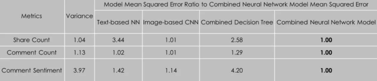
1.Text-based data can be used by machine learning models to predict user interaction on social media with a mean squared error that is less than the distribution’s variance.

2.Image-based data can be used by machine learning models to predict user interac-tion on social media with a mean squared error that is less than the distribuinterac-tion’s variance.

(32)

3. Text and image-based data can be used by machine learning models to predict user interaction on social media with a mean squared error that is lower than the mean squared error produced by either the text or image-based machine learning models.

4. Text and image-based machine learning models can statistically outperform ran-dom models when predicting for greater user interaction between Facebook advertisements. Some of the reserach questions are with reference to the distribution’s variance. This relates to model training. Models perform regression and train with a loss function. The study used mean-squared-error to calculate model loss. The formula for the mean squared error is similar the variance formula. The variance is the mean squared error with respect to the mean. This makes the variance a good baseline for understanding model performance. A model with a loss less than the variance is performing better than predicting the mean.

(33)

Chapter 4

Research Methodology

4.1

Data Context

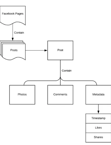
The data context consists of an online post and its metadata. The general form of content that users interact with is the online post. Posts generally contain text and might also contain an image. These posts also contain metadata. Metadata about these posts consists of likes, shares, reactions, tags, and timestamp data. A lot of this metadata are ways users have interacted with the post, e.g. by manually leaving a comment, like, reaction, or sharing the post with other Facebook users (Azizian 2017). The collected Facebook post data was drawn from advertiser Facebook pages. These pages include page data like ratings, the number of followers, and the number of persons actively speaking about the page. The combination of page data, its posts, the post data, and its comments were all collected for the study.

(34)

Figure 4.1: Data Extraction Pipeline

restricted by Facebook’s privacy policy (https://www.facebook.com/policy.php). Re-stricted interactions include likes and reactions. User Facebook pages are by default re-stricted. This left the app without access to user data.

4.1.1 Data Origin

The Facebook post URLs were obtained from AdEspresso. The website is owned by Hoot-suite, a social media management platform that was created in 2008 (Hootsuite). The company manages many platforms, including Twitter, Facebook, Instagram, LinkedIn, Google+, and YouTube (Hootsuite). The AdEspresso website provides a management

(35)

platform for social media advertising. It allows marketers to create and promote adver-tisements. The website pushes these advertisements to multiple social media platforms. The result is a single place where marketers can create and promote advertisements. The website also offers consulting for creating successful advertisements. The website features over one-hundred-thousand demo Facebook advertisements. This paper scraped these demo advertisements.

4.1.2 Collection

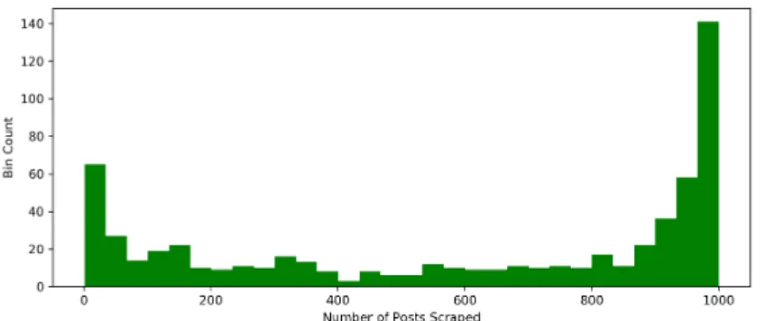
The research created a Python web scraper to crawled through these Facebook pages. All Facebook crawling was done with the Facebook’s publicly available graph API. Each Facebook page contained anywhere from a dozen to a few thousand posts. A maximum of one-thousand posts was scraped from each page. The maximum of one-thousand posts was chosen in order to control the machine learning bias to any one Facebook page. The maximum was also chosen because Facebook limits the number of API requests per day per Facebook page. Requesting content for 1000 posts and their comments can reach this limit. The full number of posts collected was over three-hundred thousand. The image URLs are stored, rather than downloaded, to save space. The text data is collected and stored in a database. Figure 4.1 shows the entire data extraction pipeline. Figure 4.2 shows a histogram of the number of posts scraped from each Facebook page.

The Facebook API is simple to use decode. Moreover, the API is hierarchical, so that the URL can be extended in order to access children elements. For example, from a Facebook page, its posts can be accessed by appending ”/Posts” to the URL. From a post URL, its comments can be accessed by appending /Comments to the URL. This made collecting data easy and less error-prone. The entire URL is also a unique hash to the page’s

(36)

Figure 4.2: Histogram of the Number of Posts Scraped Per Facebook Page

Figure 4.3: Comment Count Histogram

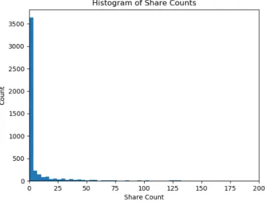
element. This makes the URL a useful primary key in the database. The sample size for share and comment counts is about 350k, and 50k samples for comment sentiment. Below are histograms in Figure 4.3-4.5 of the user interaction metrics collected for this study. The histogram sample sizes were chosen to help visualize the data.

4.1.3 Analysis Methods

Gathering data included image processing. Part of image processing is denoising images in order to emphasize important image features. The features deemed important vary for each denoising algorithm. Generally, the denoising algorithms emphasize edges, gradient

(37)

Figure 4.4: Share Count Histogram

Figure 4.5: Comment Sentiment Histogram

contrasts, and curves (Derpanis 2004). One result of denoising can be a decreased in the amount of image data, which saves computer space. The reduction in image size makes storing all the images on a machine more practical. While reducing data size is helpful, the ultimate goal is not reducing image size. The ultimate goal is eliminating image noise that might interfere with image-based model training. By eliminating noise, the models can focus on image aspects that denoising has emphasized.

(38)

Part of denoising is preparing the image for analysis. Many of the machine learning models require for all images to be the same size. Therefore, reducing image size is im-portant for the final machine learning model. One goal is to reduce image size without losing important data. One way to reduce image size while preserving important features is via seam carving (Zelinsky 2009). Seam carving is the process of resizing an image by duplicating or removing the least descriptive parts. The least descriptive parts are deter-mined by finding seams across the image where the gradient changes the least. This seam is duplicated or removed as a way of changing the image’s size. This process is a very intensive computer operation. The conclusion is that this operation was too time intensive. A fifty-pixel increase or decrease in size required a few minutes. This is far too much time when considering hundreds of thousands of images. A less sophisticated resizing method from OpenCV was instead used. Python contains a wrapper around the OpenCV C++ library for image processing. The cv2 library performs image resizing and grayscaling. The grayscale image is still noisy and needs to be processed.

A step to eliminate unimportant data is to reduce the number of image dimensions via dimensionality reduction. This can be done via principal component analysis. The number of dimensions to keep was set at 20 since the image variance is lower after denoising. This reduces noise, and data size.

Image denoising can further reduce noise. The most common type of image denoising is a Gaussian blurring. This applies image blurring and emphasizes edges. The research applied a Gaussian blur with a standard deviation of five to each image. A dilation and erosion are also applied to the image.

Basic feature detection was then applied to each image. The algorithm detects image keypoints. These keypoints are based on an image’s grayscale intensity gradient. These

(39)

keypoints were stored within a database and used to find images with similar keypoints. The final image data consists of denoised photos and their keypoints descriptors.

4.2

Text Processing

Neural networks take feature vectors as input. Yet, plain text data can not be processed by the neural network. Therefore, the research must transform the text data into vectors that are usable by the neural network. The process for transforming the text data into a word vector follows examples from ”Deep Learning with Keras” (Antonio et al., 2017). The program split the text data into words using whitespace as a delimiter. Word tokens are create from the split strings. The program grouped these tokens into sentences. The words are then lowercased and the stopwords are removed. Words with length at or below three are removed. A port stemmer is used to create stems for all the words. A POS tag library was used to perform parts-of-speech tagging. The program then extracted stems with a word lemmatizer, which takes as input the stem and the POS tag. The program fed the lemmatized text sentences to a td-IDF vectorizer. This created word vectors. The word vectors form the features for the neural network.

4.3

Open Sourced Data

The code and data have been open-sourced. The scripts have been written in Python and

stored on GitHub athttps://github.com/cpluspluscrowe/Success-Predictor-for-Social-Media-Advertisements. Hopefully, this encourages data access and use. The raw data has been included too, which

(40)

desire is that making the code available allows other researchers to adopt, replicate, and expand upon this paper’s research.

(41)

Chapter 5

Model Methodology

5.1

Data Verification

With the data collected, this research can move to the next step of building the machine learning models. This research used the collected data as model input. The input features consist of transformed text and image data. The transformed text data are the word vectors and processed images. The goal is to use the word vectors and processed images as model features to train the machine learning models.

This research tested inputs features to maximize training results. Word vector lengths from 100-100,000 are tested on text-based NNs. Word vector sizes of 10,000 produced the lowest losses. This word vector size is used throughout the study. Rectangular image sizes from 30 to 360 pixels are tested. Similar training losses on CNNs are produced for 60x60 images with regards to larger images. 60 pixels produces a CNN that trains far faster, so this size is used in all CNN models. The features were tested on smaller subsets of data that ranged from 20k-50k images. Smaller training sets were used since they are faster to train.

(42)

Once the features are selected, the model’s size and characteristics can be trained. The characteristics of a model are known as hyperparameters (Casari 2017). Badly tuned hyperparameters might produce models that do not train well (Casari 2017). For example, a large learning rate or momentum could hamper a model’s ability to converge to the solution. A high number of hidden layers could cause training overfitting and poor performance. A lack of regularization could also lead to model overfit or an odd distribution of weights within the neural network and correlated inputs. A large filter size for convolutional neural networks can cause a failure to extract image features.

Each Facebook page has auxiliary page metrics that describes how many persons follow the page and its popularity. This research used linear models to test the usefulness of these features. The wonderful thing about linear models is that they are much faster to train. The better features will increase model performance. The quick feedback is useful for identifying performant features. Yet, the Facebook page metrics were not strongly correlated with user interaction. Due to the low correlation with user engagement, the Facebook page metrics were not included as input features.

5.1.1 Approach

The goal is feature extraction for machine learning. This application includes the scaling, normalization, and categorization of data. After processing the input data, it is possible to create basic models. These models may range from linear to random forests to convolutional neural networks. Certain data are better processed by particular models (Krizhevsky 2012). For example, convolutional neural networks work well with images. Text-based models can represent Text by the frequency with bag-of-words or tf-IDF. The model can use word vectors to predict with Naive Bayes. The general approach will be to create simple features

(43)

from input data. Likely, creating features from machine learning models. This model stacking can create simple features. Other models can incorporate these features. The general goal will be to keep models and data simple. Simple data is easier to reason about, and simple models process data faster. The described verification techniques will produce and verify better features.

5.2

Data Mining

The program utilized the Facebook API to perform data mining. This data mining required creating a Facebook app, obtaining tokens, and querying the data. The tokens are Face-book’s form of authentication. The token is necessary for all Facebook queries. This allows Facebook to control content access. The application requests are throttled on an hourly and daily rate, so as to limit how many API requests occur at once. The API also throttles based upon the number of users on the application. The application created for this study was not for public use, so it had more strict API limits.

The application to collect AdExpresso links is Selenium based. It navigated the web-site by executing JavaScript to navigate to new pages. The Selenium application collected advertisement links. The website is not navigable via URLs, and all requests have au-thentication tokens. The application manually navigated through one-thousand pages on AdEspresso. The application stored the list of visited pages and skipped these whenever the application crashed. The application pickled these page numbers into a shared file and up to 20 Selenium instances were ran at once. The database only stores unique ad links, so duplicate urls causes no harm to the data. Examples of the pickle files are on GitHub with the .pkl file extension.

(44)

Figure 5.1: Data Collection Pipeline

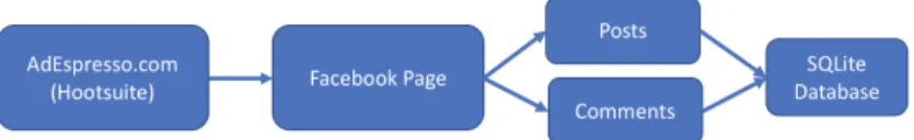
The next application converted gathered Facebook links from Expresso pages. The first application gathered links to Expresso pages, which contain Facebook links. This application visited those pages and extracted the Facebook page links. This application did not rely on executing JavaScript. Instead, Python’s urllib library retrieved the data. Python makes requests, which return the page data. The Python program then parses the request’s HTML data. The program extracted links from the HTML page. Requesting is largely I/O, so this researchers threaded the application. This application was able very stable and would run for days. The application obtained 281,090 unique Facebook page links. Figure 5.1 shows the data collection pipeline.

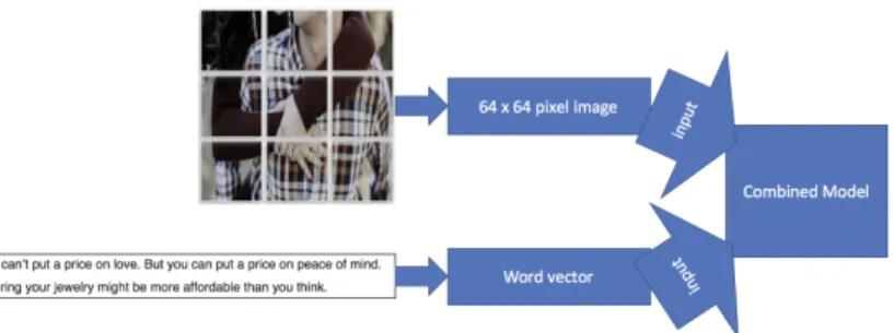
Once the application obtains Facebook links, it can scrape the Facebook pages. The third application ran through all the Facebook URLs and scraped the post data from each Facebook page. Collected post data included the post’s text, image, share count, and the number of comments. The program stores the data in a database. This is the brunt of the application and represents most of the data in the analysis. The only data missing were the Facebook comments for each post. The last Facebook post data collection application obtained comment data for each Facebook post. The application requested the comment data for each Facebook post. The comments were then stored on a database. The machine learning models used this data to learn the training data. Figure 5.2 depicts the inputs to the machine learning models.

Mark Zuckerberg testified before congress concerning the Cambridge Analytica data breach while this research was collecting Facebook data. Facebook’s immediate response

(45)

Figure 5.2: Combined Model Inputs

was to permanently disable API tokens and severely decrease the API limit threshold. These changes became large hurdles for this research to overcome. This research spent a great deal of time retrieving temporary API tokens via selenium and working with new API limitations. The study was able to overcome API throttling through threading. A single thread-safe queue stored URLs to scrape. Threads would pull from the thread-safe queue, perform work, and sleep if they hit API limitations. This allowed applications to continually run and process data as Facebook allowed. The application found that fifty threads were a good balance of scraping enough data while avoiding request throttling.

The application ran into other issues. Sometimes requests returned characters that SQLite could not store, though SQLite supports UTF-8. All these issues caused the appli-cation to run many times. The program incorporated a lot of logic to skip over already-processed data. Many of the data database layers would run queries to only return unpro-cessed Facebook links. Each application had this preprocessing layer to prevent re-obtaining old data. Moreover, if the program reprocessed old data, the storing algorithms included the insert or replace queries to exclude duplicate rows from forming within the database.

The Facebook post data included image URLs. One of the applications downloads these Facebook images. This program utilizes the urllib Python module to retrieve the image. The library implements image-processing in C and is very fast and even thread-safe. Python releases the GIL (Global Interpreter Lock) on I/O operations. The allowed the request

(46)

to perform multithreading. This makes collecting downloading many images possible in Python. Unfortunately, these images are large and require too much space. The process of downloading all the Facebook post images is impractical from a space perspective. Rather, the program must download each image. The program must immediately be processed and only store the necessary data. This process consists of three scripts. The scripts downloaded the data, denoised the data, and obtained keypoint data.

The study collected and stored user interaction data in an SQLite database. This made it possible to SCP the database between servers. The stored analysis data included Facebook post and comment data. This research stored the Facebook post data in a flat table. It included basic post information like the image’s URL, UUID, and the post’s text. The Facebook post table also included other auxiliary data so that all the data could be easily fed into a machine learning model without any joins. Some auxiliary data includes page metrics like fan count, the number of page ratings, the overall average page rating, and the number of persons talking about the page. Other calculated metrics within the table include comment count and the post’s text subjectivity. This research generated the sentiment metrics using Python’s Vader library. The library performed on social media posts. The comment table was simpler and only stored the comment’s text and its Facebook post id. The models trained on this data.

The study performed initial statistic analysis on the user interaction data. Researchers used R programming to measure the data’s distribution. Comment and share count closely fit a gamma or Weibull distribution. Figure 5.3 depicts some basic statistical fits to com-ment counts and the gamma distribution. Comcom-ment senticom-ment was similar to a normal distribution, as seen in Figure 5.4.

(47)

Empirical and theoretical dens. Data Density 0 1 2 3 4 5 0.0 0.5 1.0 1.5 0.0 0.2 0.4 0.6 0.8 1.0 1.2 0 1 2 3 4 5 Q−Q plot Theoretical quantiles Empir ical quantiles 0 1 2 3 4 5 0.0 0.2 0.4 0.6 0.8 1.0

Empirical and theoretical CDFs

Data CDF 0.2 0.4 0.6 0.8 1.0 0.0 0.2 0.4 0.6 0.8 1.0 P−P plot Theoretical probabilities Empir ical probabilities

Figure 5.3: Statistical Graphs for Comment Counts vs Gamma Distribution

5.3

Sentiment Analysis

This research used existing sentiment analysis tools to calculate sentiment for the post and comment data. Initial research began with Python’s Blob library but soon switched to using the VADER Python library. VADER (Valence Aware Dictionary and sEntiment Reasoner) is a lexicon and rule-based sentiment analysis tool that is specifically attuned to sentiments expressed in social media and works well on texts from other domains (Hutton et al., 2014). The library calculated polarity scores for the post and comment data. The comment data’s polarity scores were the output for the comment sentiment model.

(48)

Figure 5.4: Positive Comment Sentiment fit to a Normal Distribution

5.4

Algorithm Reliability

Standards exist for measuring model reliability. Model reliability describes how well the model can train, learn, and handle data variances. A more reliable model will be well suited for its data. A well suited model is quicker to trains and more sturdy to variations in the data. K-fold cross validation can measure model performance and sturdiness to small data variations (Casari 2017). This procedure trains k models, where each model uses one of the k groups as the test dataset, and the other nine as the training data. The model performance is averaged across all k data sets. Using k-fold cross validation demonstrates that the model can generalize its predictions and learn on with different sets of data. Methods like cross-validation help with data quality and prevent overfitting. This experiment used a 10-fold cross-validation on all NN and CNN models. Model training will also include types of regularization. The dropout rate also regularizes the machine learning models. A dropout of 0.35 to 0.1 is incorporated after each CNN or NN layer. Type L1 or L2

(49)

regularization can change neural network weights to prevent overfitting (Srivastava 2014). The NNs incorporate L2 regularization on each dense layer. The use of cross-validation and testing final performance on a validation test set largely ensure model reliability.

Keras provides APIs for model k-fold cross-validation. Keras is an open-source machine learning library (Keras). The models use default train-test splits. Models train to 100 epochs. The models in this research tended to begin overfitting after 30 epochs. The training began with larger batch sizes of 256. The program retrained with a larger batch size every 20 epochs. The batch sizes used were 256, 128, 64, 32, and 1. Regularization was also employed. Each NN layer includes L2 regularization. The L2 regularization had a weight penalty of 0.01. This penalty is also known as weight decay, or Ridge (Keras). Each layer also included dropouts. The dropout ranged from 0.4 to 0.1. The general pattern began with a large dropout and decrease dropout through later layers. Despite this regularization, the models eventually overtrain. Future work should include adding L1 regularization.

The process evaluates the model with the validation set. This set is a separate data set from the training and test data. The API used this dataset to check model performance. In practice, it is possible to overfit to the test set by modifying and selecting the models which have the highest test accuracy. Unfortunately, this is likely overfitting to the test set and does not represent true performance. It more accurate to test the model on a new set of data. This research set aside a third validation data set to test the final model’s performance.

(50)

5.5

Evaluation Criteria

Machine learning often takes one of two approaches, classification or regression. This re-search created regression models since the metric outputs were continuous. The values it predicts are share count, comment count, and comment polarity. The model predicts how much of these metrics the advertisement will receive. The prediction leaves advertisers with a better sense of how well their advertisement should perform on social media. The regres-sion numbers also demonstrate that the model learned the data. Thus, the regresregres-sion serves as a check to see if the model was successful at learning the data. The binary prediction for which of two ads performs best is a practical way to measure model performance.

There are existing benchmarks for predicting user interaction on social media (Straton et.all 2015). Yet, the study performs classification, not regression. The study split the Facebook posts into three ordinal groups, based on how much user interaction they received. The study then trains to classify the data into these groups. The study had a very high accuracy predicting for low user interaction. This outcome matches the zero-skewed user interaction distribution. The study did not show that their results were better than random guessing. Moreover, the classifier performed very poorly on predicting posts with more user interaction (below 10%). This study will serve as a new benchmark for performing regression on user interacti