STABILITY OF LOAD BALANCING ALGORITHMS IN
DYNAMIC ADVERSARIAL SYSTEMS∗
ELLIOT ANSHELEVICH†, DAVID KEMPE‡, AND JON KLEINBERG§
Abstract. In the dynamic load balancing problem, we seek to keep the job load roughly evenly distributed among the processors of a given network. The arrival and departure of jobs is modeled by an adversary restricted in its power. Muthukrishnan and Rajaraman [An adversarial model for distributed dynamic load balancing, in Proceedings of the 10th ACM Symposium on Parallel Algorithms and Architectures, ACM, New York, 1998] gave a clean characterization of a restriction on the adversary that can be considered the natural analogue of a cut condition. They proved that a simple local balancing algorithm proposed by Aiello et al. [Approximate load balancing on dynamic and asynchronous networks, in Proceedings of the 25th ACM Symposium on Theory of Computing, ACM, New York, 1993] is stable against such an adversary if the insertion rate is restricted to a (1−ε) fraction of the cut size. They left as an open question whether the algorithm is stable at rate 1. In this paper, we resolve this question positively, by proving stability of the local algorithm at rate 1. Our proof techniques are very different from the ones used by Muthukrishnan and Rajaraman and yield a simpler proof and tighter bounds on the difference in loads. In addition, we introduce a multicommodity version of this load balancing model and show how to extend the result to the case of balancing two different kinds of loads at once (obtaining as a corollary a new proof of the 2-commodity Max-Flow Min-Cut Theorem). We also show how to apply the proof techniques to the problem of routing packets in adversarial systems. Awerbuch et al. [Simple routing strategies for adversarial systems, in Proceedings of the 42nd IEEE Symposium on Foundations of Computer Science, IEEE Computer Society, Los Alamitos, CA, 2001] showed that the same load balancing algorithm is stable against an adversary, inserting packets at rate 1 with a single destination in dynamically changing networks. Our techniques give a much simpler proof for a different model of adversarially changing networks.
Key words. adversarial load balancing, packet routing, multicommodity flow
AMS subject classifications. 68W15, 68W40
DOI.10.1137/050639272
1. Introduction.
Load balancing. In a distributed network of computing hosts, the performance of the system can depend crucially on dividing up work effectively across the partici-pating nodes. This type ofload balancing problemhas been studied in many different models, centered around the idea that an algorithm should avoid creating “hot spots” that degrade system performance [26].
We consider a basic model of load balancing in a distributed network, which has formed the basis of a number of earlier studies [1, 18, 6, 23, 24]. A network of identical processors is represented by an undirected graphG= (V, E). There are a number of ∗Received by the editors August 31, 2005; accepted for publication (in revised form) August 14, 2007; published electronically February 14, 2008. A preliminary version of this paper appeared in
Proceedings of the34th Annual ACM Symposium on Theory of Computing, ACM, New York, 2002. http://www.siam.org/journals/sicomp/37-5/63927.html
†Department of Computer Science, Rensselaer Polytechnic Institute, Troy, NY 12180 (eanshel@ cs.rpi.edu). This author’s research was supported in part by an NSF graduate fellowship.
‡Department of Computer Science, University of Southern California, Los Angeles, CA 90089 ([email protected]). This author’s research was supported by an NSF graduate fellowship.
§Department of Computer Science, Cornell University, Ithaca, NY 14853 ([email protected]. edu). This author’s research was supported in part by a David and Lucile Packard Foundation Fellowship, an ONR Young Investigator Award, and NSF Faculty Early Career Development Award CCR-9701399.
jobs to be processed in the system, abstractly represented by unit-sizetokens. Time progresses in discrete steps calledrounds; in a given round, each token is held by one of the nodes, which is viewed as processing the associated job, and theload on a node is defined to be the number of tokens it holds. The goal is tobalancethe loads, so that no single node has too many tokens; this can be accomplished by transmitting tokens between neighboring nodes of the graph, at a rate of one token per edge per round. We are particularly interested inlocal algorithms for this problem: rather than using a centralized approach to coordinate the movement of tokens, each node will simply compare its load to those of its neighbors, and decide whether to move a token across an edge based on this information.
This model is clearly very simple in a number of respects, particularly in the uniformity of the processors (nodes) and jobs (tokens), and the fact that any job can be executed on any processor. More subtly, it is not even clear in all settings that balancing the load evenly is the optimal strategy in a distributed network of processors (see, e.g., [13]). At the same time, however, the model cleanly captures the basic constraints imposed by an underlying interconnection topology in the process of distributing jobs through a network, as evidenced by the results of previous analysis [1, 18, 6, 23, 24]; the simplicity of the model allows one to reason very clearly about the effect of these constraints.
Early work on the model focused on thestatic version of the problem: each node is given a set of tokens initially, and nodes must exchange tokens as rapidly as possible so that they all end up with approximately the same number [1, 18, 6, 24]. However, load balancing is a natural setting in which to study algorithms designed to run indefinitely; jobs (tokens) may arrive and depart from the network, and at all times, the algorithm must maintain an approximately uniform load across nodes. This is a type ofstability condition: no load should diverge arbitrarily from the average as time progresses. For a number of different models, suchdynamicalgorithms have been studied in a probabilistic framework, where one assumes an underlying randomized process that generates job arrivals and departures; see, e.g., [15, 22] and the references therein.
An adversarial model. Motivated by work in the related area of packet rout-ing [8, 9, 12, 4], Muthukrishnan and Rajaraman proposed anadversarial framework for studying dynamic load balancing in the token-based model we have been dis-cussing [23]. Rather than considering a probabilistic process that generates tokens, they posit an adversary that is allowed at the beginning of each round to introduce tokens at some nodes (corresponding to new jobs) and remove tokens from others (corresponding to jobs that have finished). Subsequently, an algorithm is allowed to move tokens across edges, as described above, so as to try to maintain balanced loads. This alternation of moves by the adversary and algorithm continues for an arbitrary number of rounds. Note that by allowing the adversary to control the removal of tokens as well as their arrival, one is modeling a worst-case assumption that jobs may have arbitrary duration, and the algorithm does not know how much processing time a job has remaining until the moment it ends.
If we letat denote the average number of tokens per node in the system at the
beginning of roundtandht(v) denote the number of tokens at nodev (theheightof v) at roundt, then the goal of a dynamic load balancing algorithm in this model is to keepht(v) close toatfor all nodesvand roundst. Formally, we say that an algorithm
isstable against a given adversary if there is a constantB such that|ht(v)−at| ≤B
deviation from the average; it is not required that the actual number of tokens in the system remain bounded.
As in the case of packet routing [12, 4], one needs to find a suitable restriction on the adversary: an arbitrarily powerful adversary could flood a particular set of nodesS⊆V with tokens much faster than these nodes can spread the tokens out to the rest of the graph, and thereby prevent any algorithm from maintaining stability. This consideration motivates the following natural definition of an adversary [23] with
rater. For a setS ⊆V, lete(S) denote the set of edges with exactly one end inS, andδt(S) the net increase in tokens in setS due to the addition and removal of jobs
in round t (note thatδt(S) could be negative). If the heights of nodes in S were to
change precisely according to the average, then the net change in tokens in S would be |S| ·(at+1−at). One wants the difference between these two quantities to be
“accounted for” by the edges ine(S). We say that the adversary hasrater if for all S⊆V, one has
(1.1) |δt(S)− |S|(at+1−at)| ≤r· |e(S)|.
For rate r >1, there are adversaries against which no algorithm (whether online or offline) can be stable. Muthukrishnan and Rajaraman gave a local-control algorithm that is stable against all adversaries of rater, for every r <1. As an open question, they asked whether there exists a local-control algorithm that is stable against all adversaries of rate 1.
The present work. We begin by providing a loccontrol load balancing al-gorithm that is stable against every adversary of rate 1, thereby resolving the open question of Muthukrishnan and Rajaraman. In fact, we show that the following simple rule has this stability property for every value of the parameterθ:
At any roundt, if the number of tokens on nodeuexceeds the number of tokens on its neighborvby at leastθ, thenumoves a token tov.
This type of algorithm was considered in earlier work on the static model by Aiello et al. [1] as well as in many subsequent papers. Settingθ= 2Δ + 1, where Δ is the maximum node degree inG, yields the specific algorithm studied by Muthukrishnan and Rajaraman.
Beyond simply showing the stability of local algorithms at thecritical rater= 1, our analysis is based on a new proof technique in which a potential function bound is maintained not only for the entire node setV but for every subset ofV. Compared to [23], we obtain significantly improved bounds on the deviation from the average, and a simpler proof. Specifically, we show that the maximum possible deviation from the average is O(Δn), where n is the number of nodes of G, and this is asymp-totically optimal in the worst case; the analysis in [23] had established a bound of O(Δ2n2.5(1−r)−1) whenr <1. Our analysis also shows stability in a more general
model where edges ofGcan appear and disappear over time.
Following this, we introduce a multicommodity version of this load balancing model. We consider a system in which there are k distinct types of jobs. The jobs of one given type induce the same load on each processor; but the different types of jobs place different resource requirements on the nodes, and so we require the load balancing condition to apply to each type separately. Formally, we have the same adversarial model as before with a networkGand a collection of tokens; but now the tokens are partitioned into k commodities and the stability requirement must hold when the tokens of each commodity are considered separately. In a single round, at most one token in total can be sent across any one edge. (This is in keeping with
the standard multicommodity notion that constraints at nodes must be satisfied by each commodity separately, while shared edge capacities must be respected by the commodities cumulatively.)
We show that the natural rate condition on adversaries—essentially obtained by summing (1.1) over the commodities—can be related in a precise sense to the cut condition for standard multicommodity network flow. As a result, applying well-known results on the cut condition [19, 20, 21], we find that for everyk >2, there is a k-commodity adversary of rate rk ≤1 against which no load balancing algorithm
can be stable.
For k = 2, however, the cut condition does not pose an obstacle to having al-gorithms that are stable all the way up to rate 1. Indeed, we are able to generalize our first result to show that for 2-commodity load balancing, there is a simple local-control algorithm that is stable against every adversary of rate 1. We also use the relationship between adversaries and cut conditions to provide a new proof of Hu’s Max-Flow Min-Cut Theorem for 2-commodity flow [19]. While our proof is not neces-sarily shorter than other proofs discovered subsequent to Hu’s [21, 25], it is arguably more elementary: it does not require linear programming duality (as in [21]) or even the traditional Max-Flow Min-Cut Theorem for single-commodity flow (as in [25]).
Finally, we further develop the connection between dynamic load balancing and network flows by extending our analysis to packet routing in the adversarial model considered by Aiello et al. [2] and Gamarnik [17]. We give an adaptive routing al-gorithm that is stable against adversaries of rate 1 in the case where packets can be injected at multiple sources but are destined for a single sink; our algorithm is stable in a dynamic network model where edges can appear and disappear. A stable algorithm for this version of the problem was previously given in a recent paper of Awerbuch et al. [7], using a different, but essentially more general, notion of a dynamic network; our proof, a direct adaptation of the analysis of our single-commodity load balancing algorithm, is considerably shorter and simpler.
Recent progress. Since the original publication of this work, several papers have studied a model wherein nodes can exchange arbitrarily many jobs in one step, and each node with a nonempty load executes one job in each time step. This type of load balancing algorithm (often called the diffusion algorithm [14]) has been very well studied and is known to have many nice properties, although its behavior in the presence of an adversary was unknown until recently. In this model, the cut condition becomes trivial; instead, the adversary is allowed to insert at mostnjobs in each time step, and stability is defined in terms of an upper bound on the load of all nodes.
Berenbrink, Friedetzky, and Goldberg [10] show that the work-stealing algorithm, in which only processors with empty queues request jobs from others, is stable against adversaries of rate strictly below 1. They assume that processors can request jobs from any other processor. Anagnostopoulos, Kirsch, and Upfal [3] show the same type of stability for a local protocol that makes nodes equalize load with their neighbors. Most recently, Berenbrink, Friedetzky, and Martin [11] proved stability against rate-1 adversaries for a protocol in which nodes exchange load with all their neighbors. Both the protocol and the analysis are very similar to those in the present work.
2. Single-commodity load balancing. In this section, we will study the load balancing problem for a single commodity and, in particular, prove that the natural balancing algorithm is stable at rate 1, thus settling an open question from [23]. We first precisely define the model and the algorithm and introduce the necessary notation.
2.1. Model and algorithm. The network is represented by a connected undi-rected graphG= (V, E) withn=|V|nodes. In each round, the adversary first adds or removes tokens (this is called theAdversary step). Subsequently, in the Redistri-bution step, up to one token can be moved along each edge e∈E by the algorithm (or up toce tokens in the case of networks with edge capacities).
The adversary is limited by the followingcut condition: For a subset S ⊆V of nodes, let δt(S),at, ande(S) be defined as above. Then, the insertion and removal
of tokens by the adversary during roundt has to satisfy (2.1) |δt(S)− |S|(at+1−at)| ≤ |e(S)|.
Nodes have queues associated with them, in which they store their tokens. The
heightht(v) of a nodevis the number of tokens inv’s queue at the beginning of round t. Theimbalance isbt(v) =ht(v)−at, i.e., the number of excess (or missing) tokens
at nodevwith respect to the average over the entire network. ht(v) andbt(v) denote
the same quantities after the Adversary step of roundt.
It is the decision of the algorithm along which edges to send tokens. The goal of any balancing algorithm is to keep the imbalance bounded for all nodes. If an algorithm ensures that there is an absolute bound B such that |bt(v)| ≤ B for all
nodes v and all times t, we call the algorithm stable. We will show that the follow-ing very simple family of local-control algorithms is stable against every adversary respecting the cut condition. It has a threshold parameterθ ≥ 1, which determines how aggressively the algorithm balances.
Algorithm SCLBθ
At each time t, for each edge e= (u, v):
If ht(u)≥ht(v) +θ, then send a token from u to v. If ht(v)≥ht(u) +θ, then send a token from v to u.
This algorithm does not specify whether tokens are sent along an edge (u, v) when
|ht(u)−ht(v)|< θ. All of our subsequent statements will remain true independently
of what the algorithm does in this case. (Notice that this algorithm requires only local information and can therefore be executed in a distributed fashion in a network.)
2.2. Stability of the algorithm. Our main theorem in this section is that the algorithm SCLBθ is stable against any adversary respecting the cut condition of inequality (2.1). We allow for tokens to be in the system at time 1 and let H := maxv∈V h1(v).
Theorem 2.1. For any adversary respecting the cut condition, and any θ ≥1, the algorithm SCLBθ is stable; i.e., there is a constantB (depending onH,θ, and G) such that |bt(v)| ≤B for all nodesv at all times t.
The intuition behind our proof is based on the (incorrect) observation that the algorithm seems to ensure that the height difference between adjacent nodes cannot grow beyond θ. Hence, the largest difference between the heights of any two nodes should be achieved whenGis a simple path, and the two nodes are the endpoints of the path—having a height difference of aboutnθ.
It is, however, easy to see that the height difference between two adjacent nodes can become more than θ, because the adversary can “rearrange” the heights within sets to a certain extent. Imagine, for instance, a long path with the adversary adding tokens to the first node of the path, until the first node has heightnθ, and the height of each successive node decreases byθ. Then it is possible to rearrange the tokens on the nodes previously having heightsnθ, (n−1)θ, and (n−2)θso that they each have (n−1)θ tokens, which would result in the height difference of 2θ between the third
and fourth nodes of the path, since the height of the fourth node remains (n−3)θ. The adversary can do this by adding two tokens to the node with height (n−2)θand subtracting one from the node with height nθ for θ successive rounds. During each Redistribution step of this process, a token will move from the third to the fourth node, but these tokens will continue traveling downhill along the path, so that the height of the fourth node will never grow to be much larger than (n−3)θ. This process obeys the cut condition, but afterward, there are two adjacent nodes with almost 2θ height difference. Fortunately, although there are now more nodes with large heights, the adversary had to pay for this rearrangement by making the highest queue smaller. In an amortized sense, the situation has not become worse.
These observations suggest maintaining height bounds for each subset of the nodes and showing that these bounds form an invariant. For convenience, we will write bt(S) =
v∈Sbt(v) for any set S ⊆V of vertices (and similarly for other quantities
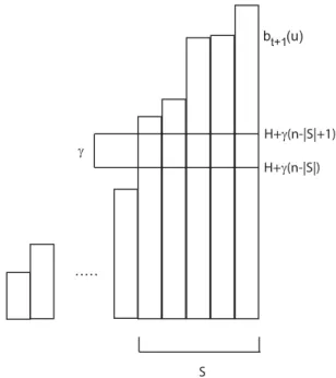
likeht(S) andδt(S)). With Δ denoting the maximum degree of any vertex, we write γ= 2Δ +θ. The key invariant is the following:
(2.2) |bt(S)| ≤
n
j=n−|S|+1
(H+γ·j) for allS⊆V.
Figure 2.1 pictorially illustrates the upper bound of this invariant as the sum of the column heights of the rightmost|S|columns.
Below, we prove Lemma 2.2, showing that inequality (2.2) is indeed an invariant over time for the algorithmSCLBθ, against any adversary respecting the cut condition.
Lemma 2.2. If the adversary respects the cut condition and the invariant (2.2) holds at the beginning of round t, then it holds at the beginning of roundt+ 1.
Using this lemma, the proof of Theorem 2.1 is straightforward.
. . . . .
|S| H
γ
1 2 n
Proof of Theorem 2.1. We prove by induction that (2.2) holds at every time t. At time 1,h1(v)≤H for allv by definition, so
|b1(S)| ≤ v∈S H ≤ n j=n−|S|+1 (H+γ·j)
for all setsS ⊆V. The induction step from t to t+ 1 follows from Lemma 2.2, and we can apply the resulting guarantee to the singleton sets{v}, yielding a bound of B=H+γ·n.
Proof of Lemma 2.2. The proof is by contradiction. Assume that the invariant (2.2) holds at the beginning of roundt but not at the beginning of round t+ 1. Let S be a set maximizing Φ(S) :=|bt+1(S)| − n j=n−|S|+1 (H+γ·j).
If several sets achieve the maximum value, let S have minimal size among all these sets. First, notice that the choice ofS guarantees that either allu∈S have positive bt+1(u), or they all have negativebt+1(u), and hence|bt+1(S)|=
u∈S|bt+1(u)|.
Since (2.2) was assumed to hold at the beginning of round t and fails at the beginning of roundt+ 1, we know that|bt+1(S)|>|bt(S)|. How can the valuesht(u)
for nodesu∈S change?
Adversary step. Substituting the definitions of b and b, we obtain that for any setS, |bt(S)|=|ht(S)− |S| ·at+1| =|ht(S) +δt(S)− |S| ·at+1| =|bt(S) +δt(S)− |S| ·(at+1−at)| ≤ |bt(S)|+|δt(S)− |S| ·(at+1−at)| ≤ |bt(S)|+|e(S)|.
The two inequalities hold because of the triangle inequality and the cut condition on the adversary.
Redistribution step. Fix an edgee = (u, v) with u ∈ S and v /∈ S. Because S maximizes Φ and has minimal size,uhas imbalance|bt+1(u)|> H+γ·(n− |S|+ 1),
since otherwise Φ(S−u)≥Φ(S). In particular,|bt+1(u)|> γ.
Because v was not included in S, its imbalance bt+1(v) must either have sign
opposite to the sign of bt+1(S) or have absolute value |bt+1(v)| ≤H +γ·(n− |S|).
In either case,|bt+1(u)−bt+1(v)|> γ, and simply substituting the definition ofγ, we
also obtain|ht+1(u)−ht+1(v)|>2Δ +θ. During the Redistribution step of roundt,
at most Δ tokens can have moved to or from nodesuandv, so their heights can have changed by at most Δ each, and therefore their previous height difference is at least
|ht(u)−ht(v)| > θ. Figure 2.2 illustrates the gap of at least γ between the queue
heights of nodes inS and outsideS.
If bt+1(u) ≥0, then ht(u)−ht(v) > θ, so the algorithm SCLBθ moves a token
from u to v along e, and no tokens from v to u, thereby decreasing bt(u) by 1.
On the other hand, if bt+1(u) < 0, then ht(v)−ht(u) > θ, and a token must be
moved fromv to ualonge, increasing the (negative) imbalancebt(u) by 1. Because
. . . . . S γ b (u)t+1 H+γ(n-|S|) H+γ(n-|S|+1)
Fig. 2.2.The gap ofγbetween the queue heights of nodes inSand outsideSin the case that bt+1(S)is positive.
not change during the Redistribution step, even if Δ tokens were moved to or from u, and hence,|bt(u)| decreased by 1 as a result of edgee.
This holds for every edgee∈e(S), and using the fact that the averageadoes not change during the Redistribution step, we obtain that
|bt+1(S)|= u∈S |bt+1(u)| ≤ u∈S |bt(u)| − |e(S)| =|bt(S)| − |e(S)|.
Putting the arguments for the two steps together, we obtain that |bt+1(S)| ≤
|bt(S)| − |e(S)| ≤ |bt(S)|. This contradicts our assumption that |bt+1(S)| > |bt(S)|
and thus completes the proof.
Notice that our boundB=H+γ·nis asymptotically tight. To see this, consider a simple path of lengthn. It is certainly legal for the adversary to insert one token at nodenin every round, and never remove tokens. After about θ·n22 rounds, each nodekwill contain aboutkθtokens, and hence the imbalance of nodenis aboutθ·n2.
2.3. Capacities, dynamic networks, and time windows. The result of The-orem 2.1 can be easily extended to the case that the edges have (integer) capacities ce associated with them, and up tocetokens can be sent alongein every round. We
assume that whenever the algorithm decides to send tokens from u to v alonge, it sends as many as possible, i.e., bounded only by the capacity ce and the number of
tokens atu. The cut condition now requires that the imbalance created by the adver-sary be restricted by the total capacity of the cut. Showing that the above algorithm
is still stable in this capacitated version is easy given Theorem 2.1.
Corollary 2.3. In the above capacitated scenario, for any adversary respecting the cut condition and anyθ≥1, the algorithmSCLBθ is stable; i.e., there is a constant B(depending onH,θ,G, and the maximum edge capacitymaxece) such that|bt(v)| ≤ B for all nodes v at all timest.
Proof. Replace each edge with capacityce byce parallel edges of capacity 1. By
Theorem 2.1, the algorithm is stable on this new graph, and therefore, it is also stable on the capacitated graph. Notice that the constant γ and hence the bound B now depend on the maximum capacity, and so instead of B = H + 2Δn+θn, the new bound becomesB=H+ 2Δn·maxece+θn, where Δ is the maximum degree of the
graph.
Dynamic networks. Another easy extension concerns dynamically changing net-works. That is, the set of available edges may change over time, and we assume that it is also controlled by the adversary. For each timet, we have a set Et of available
edges. The cut condition on the adversary must be satisfied at the specific time when the imbalance is created, i.e., |δt(S)− |S|(at+1−at)| ≤ |et(S)|. Here, et(S) are the
edges fromEt that have exactly one endpoint inS.
Corollary 2.4. In the above dynamically changing network, for any adversary respecting the cut condition, and any θ≥1, the algorithm SCLBθ is stable, i.e., there is a constant B (depending on H,θ, andG) such that |bt(v)| ≤B for all nodes v at all timest.
Proof. By syntactically replacing all terms e(S) with et(S) in the proof of
Lemma 2.2, we obtain a proof for the model of dynamically changing networks, with exactly the same boundB.
Time windows. An extension often considered in the contexts of load balancing or packet routing is to relax the restriction on the adversary by allowing it to violate the cut condition for a certain time, provided that it hold “in the long run.” Specifically, a
window sizeW is specified, and it is required that for any setSand any time window [t, t+W), the imbalance created on setS over that time window be bounded by the total capacity, i.e.,|(rt+=Wt −1δr(S))− |S|(at+W −at)| ≤W · |e(S)|.
Corollary 2.5. For any adversary respecting the cut condition on average over a window size W, and any θ ≥ 1, the algorithm SCLBθ is stable, i.e., there is a constant B (depending onH,θ,W, andG), such that |bt(v)| ≤B for all nodes v at all timest.
Proof. It is not difficult to see that by allowingB to depend onW, we can also extend the stability result to this model—once the imbalance grows too large on a set S, all edges e∈e(S) will be moving tokens so as to reduce the imbalance for every single round of an entire window, so that the imbalance cannot grow further.
3. Multicommodity load balancing. In the previous section, we considered the problem of balancing loads on processors where the loads were interchangeable. However, we are also interested in the case of different kinds of loads that are to be balanced simultaneously. For instance, think of jobs that have an emphasis on different resources of the machine they are running on. Balancing the different classes of jobs independently could be desirable in order to avoid processing time becoming a bottleneck on one machine and memory size an issue on another.
In the general multicommodity load balancing problem, we havekdifferent kinds of jobs (or tokens), which are stored in separate queues at the nodes. Our goal is to ensure an absolute bound on the deviation of any queue height from the average
queue height for that commodity. Each roundt is divided into the same two steps as before, the Adversary step and the Redistribution step.
In analogy to the single-commodity case, we use the following notation: For a nodevand commodityi, leth(ti)(v) be the number of tokens of commodityion node v at the beginning of round t. Similarly, a(ti), bt(i)(v),δt(i)(v),h(ti)(v), andb(ti)(v) are all defined for commodityiexactly as their single-commodity equivalents.
The algorithm will now have to choose not only when to send a token across an edge but also which of several available (and conflicting) kinds of tokens to send. Our class of algorithms is practically identical to the one from [2] and [7] and can be formalized as follows:
Algorithm MCLBθ
At each time t, for each edge e= (u, v): Choose i to maximize |h(ti)(u)−h(ti)(v)|. If h(ti)(u)≥h
(i)
t (v) +θ, then send a token of commodity i from u to v. If h(ti)(v)≥h
(i)
t (u) +θ, then send a token of commodity i from v to u.
In the case of a single commodity, this algorithm specializes toSCLBθ.
The natural analogue of the cut condition for a single commodity is to require that the adversary satisfy
(3.1)
i
|δt(i)(S)− |S|(a(ti+1) −a(ti))| ≤ |e(S)|
for all node setsS ⊆V and timest. This would require that the total imbalance for setS created by the adversary could be “balanced” along edges leavingS.
Unfortunately, inequality (3.1) is too weak a restriction—it allows the adversary to create patterns of addition and removal that cannot be balanced by any algorithm, whether offline or online. At the end of this section, we show how to use a reduc-tion from the multicommodity flow problem to create such an adversary with k≥3 commodities.
For the special casek= 2, however, the Max-Flow Min-Cut Theorem still holds, and, in fact, we can show that the cut condition is sufficient to ensure that algorithm
MCLBθ is stable.
3.1. Stability for k= 2. We letH = maxv∈V{h (1) 1 (v) +h
(2)
1 (v)}be the
max-imum height of the queues at any node at the start of the execution, and Δ the maximum degree of any vertex. This time, we defineγ slightly differently, namely, γ= 2Δ + 2θ.
Theorem 3.1. There is a constantB (depending onH,θ, andG), such that for any adversary respecting the cut condition,MCLBθ ensures |bt(i)(v)| ≤B at all times t, for all verticesv, and for commoditiesi= 1,2.
Proof. At the start of the execution,|b(1)1 (S)|+|b(2)1 (S)| ≤v∈SH, by definition of H. The key lemma, Lemma 3.2, establishes that for all S ⊆ V, times t, and commoditiesi= 1,2, (3.2) |b(1)t (S)|+|b(2)t (S)| ≤ n j=n−|S|+1 (H+γ·j).
Lemma 3.2. If (3.2) holds at the beginning of roundt, it holds at the beginning of roundt+ 1.
Proof. The proof is by contradiction. LetS be a set (of minimum size in case of ties) maximizing Φ(S) :=|b(1)t (S)|+|b(2)t (S)| − n j=n−|S|+1 (H+γ·j).
In the case of two commodities, a node might be included inSbecause it contributes a lot to the imbalance in one of the commodities, although its contribution to the other commodity might actually be negative. To capture the imbalance contribution of a node to each commodity, we define thesigned imbalance as βt(i)(v) := sgn(b(t+1i) (S))· b(ti)(v), β (i) t (v) := sgn(b (i) t+1(S))·b (i)
t (v) for every node v ∈V and every time step t.
Here, sgn denotes the sign of a term. Notice that we use the sign of b(ti+1) (S) at all time steps t in the definition ofβt(i)(v) (not the sign of b(ti)(S) or ofb
(i)
t+1(S)). We
can now rewrite the total imbalance over the setS at timet+ 1 as (3.3) |b(1)t+1(S)|+|b(2)t+1(S)|=
u∈S
(βt(1)+1(u) +β(2)t+1(u)).
Again, we show that the change in the imbalance for set S cannot be positive, by comparing the increase in the imbalance ofS during the Adversary step with the decrease during the Redistribution step, and thus obtain a contradiction.
Adversary step. We know that for each commodityi= 1,2, the imbalance on set Safter the Adversary step is at most|b(ti)(S)| ≤ |b
(i) t (S)|+|δ (i) t (S)− |S| ·(a (i) t+1−a (i) t )|
by the triangle inequality. Now, summing overi= 1,2 and applying the cut condition on the adversary yield that
|b(1)t (S)|+|b(2)t (S)| ≤ |b(1)t (S)|+|b(2)t (S)|+|e(S)|.
Redistribution step. Fix a node u∈S, and an edgee= (u, v) of Gwith v /∈S. As in the proof of Lemma 2.2, we can use the definition of S (as maximizing Φ and being of minimal size) to obtain that the signed imbalances at nodesuandv satisfy βt(1)+1(u) +βt(2)+1(u)> βt(1)+1(v) +βt(2)+1(v) +γ. Asuandv can lose and gain at most Δ tokens each during the Redistribution step,
(3.4) β(1)t (u) +β (2) t (u)> β (1) t (v) +β (2) t (v) + 2θ.
In particular, there must be a commodity isuch thatβ(ti)(u)> β(ti)(v) +θ, and thus also|h(ti)(u)−h
(i)
t (v)|> θ. Hence,MCLBθmoved a token along edgeeduring the
Redistribution step (w.l.o.g., it was a token of commodity 1). We want to show that this token actually decreased the signed imbalance of nodeu. Assume that it did not. This means that if the token moved fromutov, then sgn(b(1)t+1(S)) is negative, and if the token moved fromv tou, then sgn(b(1)t+1(S)) is positive. In either case, the signed imbalance for commodity 1 at nodev must be higher than at node u, and so
BecauseMCLBθmaximizes the difference in its choice of commodity, we obtain that β(1)t (v)−β(1)t (u) =|h(1)t (v)−h(1)t (u)| ≥ |h(2)t (v)−h(2)t (u)| =|β(2)t (v)−β (2) t (u)| ≥β(2)t (u)−β(2)t (v). Rearranging this inequality yields that
β(1)t (v) +β(2)t (v)≥β(1)t (u) +β(2)t (u)
and thus results in a contradiction with inequality (3.4). Therefore, every edge (u, v) withv /∈S decreases the signed imbalance ofuby 1. Summing over all edges and all nodesu∈Sgives usβt(1)+1(S) +β(2)t+1(S)≤β(1)t (S) +β(2)t (S)− |e(S)|. Using (3.3) and the fact thatβ(1)t (S) +β
(2) t (S)≤ |b (1) t (S)|+|b (2) t (S)|, we obtain|b (1) t+1(S)|+|b (2) t+1(S)| ≤ |b(1)t (S)|+|b(2)t (S)| − |e(S)|.
Combining the arguments for the two steps |b(1)t (S)|+|b(2)t (S)| increases by at most |e(S)| during the Adversary step and decreases by at least |e(S)| during the Redistribution step. Therefore, in total |b(1)t+1(S)|+|b(2)t+1(S)| ≤ |b(1)t (S)|+|b
(2) t (S)|,
which is a contradiction.
The result for two commodities can be extended to networks with edge capacities, adversarially changing edge sets, and adversaries with restrictions only for larger window sizes, just like for the single-commodity case.
3.2. Load balancing and flows. By omitting the adversarial and dynamic nature in the load balancing problem, and forcing the adversary to repeat the same pattern of token additions in every round, we can infer from the stability of the load balancing algorithm the existence of a multicommodity flow. Suppose that we are given a multicommodity flow instance with edge capacities ce, source-sink pairs
(si, ti), and demandsdi. LetD = maxidi, and let A be the adversary inserting, in
every round and for each commodity i, D+di tokens at nodesi, D−di tokens at
nodeti, and Dtokens everywhere else.
Lemma 3.3. If there is a load balancing algorithm that is stable against the adversaryA, then there is a (fractional) multicommodity flowf with source-sink pairs
(si, ti)and demandsdi.
Proof. Because we assumed the algorithm to be stable, all imbalancesb(ti)(v) are always bounded in absolute value by some constantB. Therefore, there are at most (2B+ 1)kn different combinations of imbalances for the entire network, and so there
must exist two time steps tand t such thatt < t and bt(i)(v) =b(ti)(v) for all nodes
v and commoditiesi.
For each edgee= (u, v), letσr(i)(u, v) denote the number of tokens of commodity isent fromutov in roundr, and define a flowf by
f((u,vi) ):= 1 t−t·
t−1
r=t
(σr(i)(u, v)−σr(i)(v, u)).
Notice that we define negative flows, but only for symmetry and ease of notation. We want to verify thatf is indeed a feasible multicommodity flow for demands (si, ti, di).
Capacity constraints. The total flow along any edge (u, v) is i |f((u,vi) )| ≤ 1 t−t · i t−1 r=t |σ(ri)(u, v)−σ(ri)(v, u)| = 1 t−t · t−1 r=t i |σ(ri)(u, v)−σ(ri)(v, u)| ≤ 1 t−t · t−1 r=t c(u,v) =c(u,v).
The first inequality is simply the triangle inequality, and the second inequality holds because the balancing algorithm never exceeds the capacity of any edge with any of its token moves, and therefore bothσ(ri)(u, v) andσ
(i)
r (v, u) lie between 0 andc(u,v). Flow conservation. For any nodev and commodityi, we can write
(t−t) (u,v)∈E f((u,vi) ) = (u,v)∈E t−1 r=t (σ(ri)(u, v)−σr(i)(v, u)) = t−1 r=t (u,v)∈E σ(ri)(u, v)− t−1 r=t (u,v)∈E σr(i)(v, u) =h(ti)(v)−h (i) t (v)− t−1 r=t δ(ri)(v) =b(ti)(v) +a(ti)−b (i) t (v)−a (i) t −(t−t)·δ (i) t (v) = (t−t)(D−δ(ti)(v)).
The third equality is true because h(ti)(v)−h(ti)(v) is exactly the number of tokens
that enteredvduring the time period [t, t−1], minus the number of tokens that left vduring this period. In the last equality, we used thatb(ti)(v) =b
(i)
t (v) for alliandv,
and thata(ri)=r·Dfor all timesr. Now, if nodevis neither the source nor the sink for
commodityi, thenδt(i)(v) =D, so flow is conserved. If v is the source of commodity i, thenδt(i)(v) =D+di, so the total flow entering nodesi is−di. Ifvis the sink for
commodityi, then the total flow entering node ti isdi, because δ (i)
t (v) =D−di by
definition. Hence,f satisfies flow conservation and all demands.
f conserves flow, satisfies all demands, and does not exceed any edge capacities, so it is a feasible multicommodity flow for the given demands.
By combining Lemma 3.3 with the stability of MCLBθ proved in Theorem 3.1, we obtain as a corollary an alternate proof of the 2-commodity Max-Flow Min-Cut Theorem. It remains only to verify that the adversary A as defined in Lemma 3.3 indeed respects the cut condition.
Corollary 3.4 (2-commodity Max-Flow Min-Cut). LetG= (V, E) be a graph with edge capacities ce and two demand pairs (s1, t1), (s2, t2) with demands d1, d2
such that for any vertex set S ⊆ V, the total demand of commodities i ∈ {1,2}
with exactly one of {si, ti} in S is at most
e∈e(S)ce. Then, there exists a feasible
2-commodity flow sending di units of flow fromsi toti fori= 1,2.
Proof. Define the adversary A as in Lemma 3.3. To show that the algorithm
MCLBθ is stable againstA, we merely have to verify thatAsatisfies the cut condition. Let S ⊆ V be arbitrary. For convenience, we write [u ∈ S] := 1 if u ∈ S, and 0 otherwise. Then, for any timet
i=1,2 |δt(i)(S)− |S| ·(a(ti+1) −a(ti))| = i=1,2 ||S| ·D+ [si∈S]·di−[ti∈S]·di− |S| ·D| = i=1,2 di· |[si ∈S]−[ti∈S]|.
In the first equality, we used the definition of the insertion pattern for A. The con-tribution of commodity i to this sum isdi if and only if exactly one ofsi, ti lies in S—otherwise, it is 0. Hence, the value of the sum is the total demand of commodities i with exactly one of {si, ti} in S, which by assumption is bounded by
e∈e(S)ce.
Hence,Asatisfies the cut condition.
We can therefore apply Theorem 3.1 to obtain that MCLBθ is stable against A, which in turn implies the existence of a feasible multicommodity flowf for the given instance via Lemma 3.3.
The 2-commodity Max-Flow Min-Cut Theorem was first proved by Hu [19], es-sentially repeating Ford and Fulkerson’s original [16] augmenting paths argument for two commodities. Seymour [25] showed a short and simple explicit reduction to the single-commodity case. Subsequently, Linial, London, and Rabinovich [21] gave a novel proof using geometric embeddings and linear programming duality. Our proof uses yet different (and much more elementary) techniques and does not rely on the single-commodity Max-Flow Min-Cut Theorem.
Another corollary we obtain from Lemma 3.3 is the existence of an adversary respecting the cut condition for k= 3 commodities, such that no algorithm (offline or online) can balance the insertion pattern. This is not surprising, since load bal-ancing algorithms (and our algorithm, in particular) attempt to generate a flow from overloaded nodes to underloaded nodes, and we know that the best flows can be significantly worse than the best cuts for more than two commodities (i.e., the Max-Flow Min-Cut Theorem does not hold fork≥3). This means that the constraint on the adversary is not powerful enough to guarantee the existence of a good flow and therefore a good algorithm. We make the above discussion precise in the following corollary.
Corollary 3.5. There exists an adversary respecting the cut condition fork= 3 commodities, such that no algorithm (offline or online) is stable against this adver-sary.
Proof. To prove this, we simply take a 3-commodity instance with a graphG= (V, E) and demand pairs (si, ti),i∈ {1,2,3}(with demandsdi), such that for all cuts
(S, V\S), the total demand across the cut is at most the capacity of the edges crossing the cut, yet there is no (fractional) multicommodity flow satisfying all demands. The first such example for k = 3 was given in [19]. (A simpler well-known example for k= 4 is the complete bipartite graphK2,3 with a unit demand between every pair of
nodes that are at a distance of 2 from each other.) Let Abe the adversary defined from this instance as in Lemma 3.3. If any load balancing algorithm were stable against A, Lemma 3.3 would guarantee a feasible multicommodity flow, which is a contradiction.
The above corollary and Lemma 3.3 illustrate the relation of multicommodity flows to load balancing algorithms and tell us that the cut condition is not enough to guarantee the existence of a stable algorithm for k≥3. In section 5, we will discuss an alternative approach for a restriction on a multicommodity adversary.
4. Packet routing. There is a natural connection between the load balancing problem studied in the previous sections and the problem of routing packets in an adversarial network. It has been observed previously [2, 7] that the natural balancing algorithmSCLBθis also stable for packet routing.
The model for packet routing differs from the load balancing one in that after the Redistribution step, there is an additionalRemoval step, during which all packets which have reached their destination are removed from the network. Stability of an algorithm is now defined as meaning that there is an absolute bound on all queue heights at all times, i.e.,h(ti)(v)≤B for some constantB.
In the single-commodity packet routing problem, we can again restrict the adver-sary by a cut condition: the total numberδt(S) of packets inserted into a setSmust
be at most|e(S)|for any setS not containing the sink of the packets. IfSdoes con-tain the sink, then there is no restriction. In the multicommodity case, the adversary specifies a source si and a sink ti for each packet inserted and must guarantee that
there is a set of edge-disjoint paths connecting all (si,ti) pairs.
In [7], it was shown that for the single-commodity case, the algorithm SCLBθ
is stable against an adversary guaranteeing the existence of a path for all packets inserted, even when edges dynamically appear and disappear. Aiello et al. [2] proved that an algorithm essentially equivalent to MCLBθ is stable for the multicommodity packet routing problem if the paths specified by the adversary not only are disjoint but also leave an ε fraction of capacity for every edge unused over a given window lengthW. Recently, [5] extended this result to dynamically changing networks.
Our techniques from section 2 can be used to obtain an alternate (and simpler) proof for the stability of algorithmSCLBθin the packet routing model. Our proof also works for the case of adversarially appearing and disappearing edges, although the restriction on the adversary is different from (and essentially less general than) the one in [7].
We define Δ and H as before and letγ= 2Δ +θ. Then, the stability of SCLBθ
against an adversary respecting the cut condition is guaranteed by the following the-orem.
Theorem 4.1. For any time t and setS⊆V,
(4.1) ht(S)≤
n
j=n−|S|+1
(H+γ·j).
Proof. By definition of H, invariant (4.1) certainly holds at time 1. Assume that the theorem is wrong, and let t be the earliest time such that there is a set S violating (4.1) at time t+ 1. Among all such sets, let S be the one maximizing ht+1(S)−
n
j=n−|S|+1(H+γ·j), and break ties for minimal size. Then, we can show
andht+1(u)> H. In particular, the setS cannot contain the sink (because the sink
contains no tokens after the Removal step).
Therefore, the adversary can have inserted at most |e(S)| tokens into S in the Adversary step. During the Redistribution step of roundt, a token leaves the setS along each edge e = (u, v) ∈ e(S), because even if u had lost Δ tokens and v had gained Δ tokens during the Redistribution step, ht(u) would still exceed ht(v) by
at least θ. Taken together, this shows that the number of tokens in S cannot have increased, contradicting the choice oft andS.
Extensions. Like the proofs in the previous sections, the proof of Theorem 4.1 can be easily extended to deal with dynamically changing networks, edge capacities, and time windows in the cut condition. In addition, this proof extends to directed graphsGif we redefinee(S) in the cut condition to be the edges coming out ofS. We can also show stability for a wider class of single-commodity balancing algorithms. Specifically, let g : N → N be a function with g(x) ≥ x for all x. The balancing algorithmSCLBgalways sends a token fromutov (and never sends a token fromvto u) if there is an edgee= (u, v)∈E and ht(u)> g(ht(v)). It does not matter what
the algorithm does if neither ht(u)> g(ht(v)) nor ht(v) > g(ht(u)). Extending the
above proof only slightly, we obtain that SCLBg is stable for all such functionsg. Of course, the boundB now depends on the rate of growth ofg.
Our packet routing results also imply the stability of an interesting load balancing scenario, which is very similar to the one in [11]. Suppose that each node processes one job per round so that one token is removed in every round from each node with positive queue height. If the adversaryA satisfies the constraint that the number of tokens it adds toS be at moste(S) +|S|, then we can use Theorem 4.1 to show that the queue heights are bounded. Consider adding a sink nodev to our graph, and add an edge from every node tov. We can now think ofAas adding packets to the new graph, withvbeing the packets’ destination. The number of edges coming out of a set S in the new graph is exactly e(S) =e(S) +|S|, soAsatisfies the condition needed for Theorem 4.1. It is easy to see that if the queue heights are bounded in this new packet routing scenario, then they are also bounded in the original load balancing one.
The proofs for Theorems 4.1 and 2.1 (and the proofs in [2] and [23]) are so similar in nature that one suspects a formal reduction from the packet routing problem to the load balancing problem (which seems more general). However, we have not yet been able to determine such a reduction. It would certainly be interesting, since it would allow us to focus on the load balancing problem in the future.
As with the load balancing problem, we can obtain a multicommodity flow ifMCLBθ
is stable against a suitably defined adversaryA. The proof is practically identical to the one for Lemma 3.3, and we therefore omit it.
Lemma 4.2. Let A be an adversary inserting di tokens of commodity i (whose destination is ti) into node si in every round. If there is a routing algorithm that is stable against this adversary, then there is a (fractional) multicommodity flowf with source-sink pairs (si, ti)and demandsdi.
5. Conclusions. In this paper, we have shown that a simple local load balanc-ing algorithm is stable against dynamic adversarial addition and removal of jobs in a network, so long as the adversary is bounded by a natural extension of the cut con-dition in the sense defined in [23]. This settles an open question from [23]. Our proof techniques extend to the cases of balancing two commodities at once and to routing packets injected by an adversary. They yield easier proofs and essentially tight bounds
for the general case. In addition, the stability of the load balancing algorithm for two commodities gives a new proof of the 2-commodity Max-Flow Min-Cut Theorem.
This work leaves open a number of interesting questions. Most importantly, we would like to be able to show stability of the multicommodity load balancing algorithm for an arbitrary number of commodities, both for the problem of routing packets and balancing loads. If we want to prove the stability of load balancing algorithms for more commodities, we will have to use a different condition on the adversary. As a consequence of Lemma 3.3, any reasonable restriction on the adversary will have to guarantee the existence of multicommodity flows for all instances where we hope to prove stability. We therefore suggest the following restriction:
First, define demandsd(ti)(v) for commodityi, nodev, and timetby d(ti)(v) :=δt(i)(v)−(a(t+1i) −a(ti)). Then, the adversary is restricted to moves that guarantee the existence of a (fractional) multicommodity flow inGsatisfying all these demands.
The disadvantage of this condition is that it bears no direct relation to the load balancing problem—it arises from observing the insufficiency of the more natural cut condition rather than from having an actual meaning for the problem of balancing loads. Nevertheless, this condition should be considered the right restriction on the adversary to measure the quality ofMCLBθor other load balancing algorithms.
Alternatively, we might investigate whether the cut condition is sufficient for balancing multiple loads if we restrict our attention to specific networks. For example, it is well known that for trees or cycles, the cut condition implies the existence of multicommodity flows, and we might hope that it would hence be sufficient to prove stability.
Acknowledgments. We thank Martin P´al and Christian Scheideler for valuable discussions on the subjects of load balancing and adversarial packet routing.
REFERENCES
[1] W. Aiello, B. Awerbuch, B. Maggs, and S. Rao,Approximate load balancing on dynamic and asynchronous networks, in Proceedings of the 25th ACM Symposium on Theory of Computing, ACM, New York, 1993, pp. 632–641.
[2] W. Aiello, E. Kushilevitz, R. Ostrovsky, and A. Ros´en,Adaptive packet routing for bursty adversarial traffic, in Proceedings of the 30th ACM Symposium on Theory of Computing, ACM, New York, 1998, pp. 359–368.
[3] A. Anagnostopoulos, A. Kirsch, and E. Upfal,Load balancing in arbitrary network topolo-gies with stochastic adversarial input, SIAM J. Comput., 34 (2005), pp. 616–639. [4] D. M. Andrews, B. Awerbuch, A. Fern´andez, J. Kleinberg, F. T. Leighton, and Z. Liu,
Universal stability results for greedy contention–resolution protocols, J. ACM, 48 (2001), pp. 39–69.
[5] M. Andrews, K. Jung, and A. Stolyar,Stability of the max-weight routing and schedul-ing protocol in dynamic networks and at critical loads, in Proceedings of the 38th ACM Symposium on Theory of Computing, ACM, New York, 2007, pp. 145–154.
[6] F. Meyer auf der Heide, B. Oesterdiekhoff, and R. Wanka, Strongly adaptive token distribution, Algorithmica, 15 (1996), pp. 413–427.
[7] B. Awerbuch, P. Berenbrink, A. Brinkmann, and C. Scheideler,Simple routing strategies for adversarial systems, in Proceedings of the 42nd IEEE Symposium on Foundations of Computer Science, IEEE Computer Society, Los Alamitos, CA, 2001, pp. 158–167. [8] B. Awerbuch and F. T. Leighton,A simple local-control approximation algorithm for
multi-commodity flow, in Proceedings of the 34th IEEE Symposium on Foundations of Computer Science, IEEE Computer Society, Los Alamitos, CA, 1993, pp. 459–468.
[9] B. Awerbuch and F. T. Leighton, Improved approximation algorithms for the multi-commodity flow problem and local competitive routing in dynamic networks, in Proceedings of the 26th ACM Symposium on Theory of Computing, ACM, New York, 1994.
[10] P. Berenbrink, T. Friedetzky, and L. A. Goldberg,The natural work-stealing algorithm is stable, SIAM J. Comput., 32 (2003), pp. 1260–1279.
[11] P. Berenbrink, T. Friedetzky, and R. Martin,Dynamic diffusion load balancing, in
Pro-ceedings of the 32nd International Colloquium on Automata, Languages and Programming, Lisbon, Portugal, 2005, pp. 1386–1398.
[12] A. Borodin, J. Kleinberg, P. Raghavan, M. Sudan, and D. Williamson,Adversarial queue-ing theory, J. ACM, 48 (2001), pp. 13–38.
[13] M. Crovella, M. Harchol-Balter, and C. Murta,Task assignment in a distributed sys-tem: Improving performance by unbalancing load, in Proceedings of the ACM Sigmetrics Conference on Measurement and Modeling of Computer Systems, ACM, New York, 1998, pp. 268–269.
[14] G. Cybenko,Load balancing for distributed memory multiprocessors, J. Parallel Distrib.
Com-put., 7 (1989), pp. 279–301.
[15] D. Eager, E. Lazowska, and J. Zahorjan,Adaptive load sharing in homogeneous distributed systems, IEEE Trans. Software Engineering, 12 (1986), pp. 662–675.
[16] L. Ford and D. Fulkerson,Maximal flow through a network, Canad. J. Math., 8 (1956), pp.
399–404.
[17] D. Gamarnik,Stability of adaptive and non-adaptive packet routing policies in adversarial queueing networks, in Proceedings of the 31st ACM Symposium on Theory of Computing, ACM, New York, 1999, pp. 206–214.
[18] B. Ghosh, F. T. Leighton, B. Maggs, S. Muthukrishnan, C. Plaxton, R. Rajaraman, A. Richa, R. Tarjan, and D. Zuckerman, Tight analyses of two local load balancing algorithms, in Proceedings of the 27th ACM Symposium on Theory of Computing, ACM, New York, 1995.
[19] T. C. Hu,Multi-commodity network flows, Oper. Res., 11 (1963), pp. 344–360.
[20] F. T. Leighton and S. Rao,Multicommodity max-flow min-cut theorems and their use in designing approximation algorithms, J. ACM, 46 (1999), pp. 787–832.
[21] N. Linial, E. London, and Y. Rabinovich,The geometry of graphs and some of its algorith-mic applications, Combinatorica, 15 (1995), pp. 215–245.
[22] M. Mitzenmacher, On the analysis of randomized load balancing schemes, in Proceedings
of the 9th ACM Symposium on Parallel Algorithms and Architectures, ACM, New York, 1997, pp. 292–301.
[23] S. Muthukrishnan and R. Rajaraman,An adversarial model for distributed dynamic load balancing, in Proceedings of the 10th ACM Symposium on Parallel Algorithms and Archi-tectures, ACM, New York, 1998, pp. 47–54.
[24] D. Peleg and E. Upfal,The token distribution problem, SIAM J. Comput., 18 (1989), pp. 229–
243.
[25] P. D. Seymour,A short proof of the two-commodity flow theorem, J. Combin. Theory Ser. B,
26 (1979), pp. 370–371.
[26] B. Shirazi, A. Hurson, and K. Kavi,Scheduling and Load Balancing in Parallel and Dis-tributed Systems, IEEE Computer Society, Los Alamitos, CA, 1995.