Face beauty analysis via manifold based semi-supervised learning

(1)

Master’s Degree

Computational Engineering and Intelligent Systems

(Department of Computer Science and Artificial Intelligence)

Master thesis

Face Beauty Analysis

via Manifold based Semi-Supervised

Learning

Anne Elorza Deias

Directors

Fadi Dornaika

(2)

(3)

Acknowledgements

I would like to thank my directors, Fadi and Ignacio, for their sensible and practical advices, as well as their extraordinarily prompt responses to all my e-mails, which must not be taken for granted. My family and closest friends, who are not madly keen on science, and nonetheless listened attentively to the finest details of this work (or so did they say). I especially thank Maria, for understanding, Tonina, for trying to understand, Izaskun, for being there, Uxue, for popping up from time to time, Lierni and Gaizka, for teaching me the topology of knots and ropes, and Asier, for our nocturnal discussions about Lebesgue’s integral in neural networks.

(4)

(5)

Summary

Beauty has always played an important role in society, implicitly influencing the hu-man interactions of our daily lives and more significant aspects, such as the mate choice or job interviews. And now, with the progress made in deep learning and fea-ture extraction, automatic facial beauty analysis has become an emerging research topic too. However, the subjectivity of beauty still hinders the development in this area, due to the cost of collecting reliable labeled data, since the beauty score of an individual has to be determined according to various raters.

To address this problem, we study the performances of four different semi-supervised manifold based algorithms, which can take advantage of both labeled and unlabeled data in the training phase, and we use them in two different datasets: SCUT-FBP

and M2B. The learning algorithms are Local and Global Consistency, Flexible

Man-ifold Embedding and Kernel Flexible ManMan-ifold Embedding. There is an additional algorithm, which, unlike the rest of them, instead of performing classification, ob-tains a non-linear transformation of the data to make the classification easier. All of these algorithms were designed to work on discrete classes, but we perform regres-sion, where labels are real numbers. So the first step, in chapter 2, is to analyse how the algorithms can be adapted to regression and to hypothesize which problems we could be encountering in this process. Secondly, we empirically test them (chapter 3). The best results are obtained with KFME on both datasets, achieving a mean average error of 0.0550 (out of 1) and a Pearson correlation of 0.8446 on SCUT-FBP

dataset. With respect to M2B dataset, a mean average error of 0.1357 and a

Pear-son correlation of 0.4469 are achieved on eastern faces, while a mean average error of 0.1132 and a Pearson correlation of 0.6322 are achieved on western faces. This dissertation ends with a final chapter discussing the results and proposing new topics of study for future work.

(6)

(7)

Chapter 1

Introduction

1.1

Motivation

This work is a comparative study of manifold based semi-supervised algorithms ap-plied to the specific problem of automatic facial beauty assessment. The statement of the problem can be the following: given a facial image, what would its beauty score, ranging from 1 to 10, be? Its resolution, instead, is a highly complex matter. The main problem we will try to address is the scarcity of labeled data regarding this specific topic, which is due to its subjective nature. It is well known that beauty lies in the eye of the beholder, so obtaining reliable databases requires a great deal of human labor. In order to obtain meaningful labels, many raters are needed and, usually, the ground truth label of an image is considered to be the average score of all the ratings given by different raters. So, in this context, semi-supervised learning appears to be particularly appropriate. Unlike supervised learning, which just makes use of labeled data, this approach utilizes the information underlying the unlabeled data as well. There exist several ways of taking advantage of unlabeled samples. In our case, we have chosen graph-based methods, which, roughly speaking, work under the assumption that similar samples should share similar labels. Thinking about beauty, it seems quite reasonable to assume that when two faces resemble each other they should be similarly attractive. This abstract idea can be materialized by creating a fully-connected weighted graph, in which nodes are samples and the weights between each pair of nodes represent their similarities. Chapter 2 specifies this mechanism in greater detail.

As one can imagine, automatic beauty evaluation is not limited to exploiting as much information as one can and many other issues arise during its study. For example, a crucial aspect is which features represent best a face or, if one prefers philosophy over technicity, they may wonder whether a machine will ever be able to learn something so seemingly human as beauty perception. In the next section, a brief review will be presented, and we will see that these queries and others have already been made in the past.

(10)

10 CHAPTER 1. INTRODUCTION

1.2

Related work: Beauty analysis in computer

science

The first automatic facial beauty system [1], published in 2001, aimed at classifying beauty in 4 different classes. Each image was described by 8 ratios (e.g. the ratio of the horizontal distance between the eyes to the average vertical distance between the eyes and the mouth), which were supposed to capture the essence of beauty accord-ing to previous studies made by psychologists and biologists. This means there were only 8 features, and the performance of the classifier strongly depended on a correct localization of the eyes and the mouth. The dataset consisted of 80 photos, each of them had been rated by 12 individuals among the 4 classes, and the ground truth label was the median of all raters’ ratings. The classifyer was a variant of k-nearest neighbors.

Since then, many aspects of the research have been developed. The first accurate fa-cial attractiveness predictor [9, 10] used a high number of features: 98 image features, 90 geometric and 8 related to face simmetry, hair and skin color and skin smooth-ness. Their study, along with others [4], reinforced the idea that beauty perception is something a machine can learn. However, together with the still limited size of the dataset (around 90 images), this study still had another major flaw: the process of feature extraction was not fully automatic. In fact, the geometric features were based on landmarks. These were found by an automatic engine capable of identifying eyes, nose, lips, eyebrows, and head contour; yet some of them failed to be correctly identified and had to be adjusted manually. This drawback was firstly overcome by building a family of convolutional neural networks whose input was the raw image and the output was the score [7].

One of the principal challenges of the research in this field has been to build accu-rate facial representations, which can be either feature-based, holistic or hybrid. In the first category one can find geometric, color, texture or other local representa-tions. Geometric representations use landmark points and consider their positions, distances between them or ratios of these distances, and some of the studies have also focused on the relationship between the golden ratio and beauty [16]. On the other hand, the holistic approach uses the global information of the face, instead of local features, e.g., using eigenfaces [4]. This approach also includes recent representations learnt with deep learning [6, 21].

Since 2013, the studies in this area have partly focused on constructing larger and reliable benchmarks [13, 12, 22]. Many recent works make use of various neural networks [6, 13, 22, 23]. One paper utilizes semi-supervised learning [6]; more specif-ically, it uses deep self-taught learning. This strategy combines the semi-supervised setting with deep learning in order to extract more meaningful features, whereas the classification remains supervised.

If one wishes a thorough insight into the related work, a complete review can be found at [11].

(11)

1.3. OUR STUDY 11

1.3

Our study

The problem we will be facing will be regression, where labels belong to a continuous space, namely the interval of possible scores, rather than a restricted set of discrete classes. For this purpose we will use four semi-supervised manifold based algorithms (see chapter 2) and a couple of classical supervised algorithms to establish the

com-parison between them, all of which have been implemented in MATLAB1. The two

datasets used in the study are described below.

1.3.1

Datasets

Two different datasets are used in this work: SCUT-FBP dataset [22] and the Multi

Modality-Beauty (M2B) dataset [13]. The former was specifically designed for

auto-matic facial beauty perception and contains high resolution front-on face portraits of Asian females. On the other hand, the latter was developed to evaluate beauty via face, dressing and/or voice on both Eastern and Western females and each instance in the dataset contains information about the three modalities. However, we are only focusing on the facial images, which unlike the ones in SCUT-FBP dataset, show very different poses and expressions. This complicates, in consequence, the beauty assessment, which could be found difficult even by a human rater.

SCUT-FBP dataset

SCUT-FBP dataset contains 500 high resolution front-on face portraits of Asian females with neutral expressions, simple background and minimal occlusion, as can be seen in figure 1.1. These characteristics prevent from taking into account irrelevant factors in the beauty classification task.

The beauty rankings lie on the interval (1, 5) and are the result of averaging various ratings. The ratings were collected among 75 individuals using a web based tool, as can be seen in figure 1.2, with an average number of 70 raters per image.

The ratings aproximately follow a normal distribution (figure 1.3) with a small peak around 4.5. This suddenly high number of beautiful individuals is “artificial”. Even though in the real world beautiful faces constitute a small percentage of the popu-lation, more beautiful faces were included in the database to facilitate the beauty classification task.

Raters’ consistency and self-consistency are checked in different ways by the authors of the paper. For instance, low standard deviations in the ratings of each image indicate rater’s agreement in the perception of beauty.

1_c _{2017 The MathWorks, Inc.} _{MATLAB and Simulink are registered trademarks of The}

MathWorks, Inc. See https://es.mathworks.com/company/aboutus/policies_statements/ trademarks.html for a list of additional trademarks. Other product or brand names may be trademarks or registered trademarks of their respective holders.

(12)

12 CHAPTER 1. INTRODUCTION

Figure 1.1: Examples of face portraits of SCUT-FBP dataset from [22].

M2B dataset

The Multi-Modality Beauty dataset has been developed to study beauty perception in three different modalities, in dressing, in the face and in the voice, as well as the global beauty perceived when any of these three aspects are combined. Therefore, the dataset contains one face photo, one full body photo and one voice snippet of 1240 females belonging to two ethnic groups: westerners and easterners (620 individ-uals in each group). In addition, each of the females of the dataset is rated, in the different modalities and their combinations, with various scores in the interval [1, 10]. The ratings were collected among 40 participants, which were split into two groups depending on their ethnicity, so that each of the participants rated females of their own ethnic group. The web tool used for this purpose can be seen in figure 1.4.

The ratings were obtained usingk-wise comparison, which means that the raters are

asked to order k females according to their beauty, and then these k-wise ratings

were converted into global ratings in the interval [1, 10] by solving an optimization problem to preserve as many pairwise preferences as possible. The drawback of this method of collecting the labels is that, opposedly to SCUT-FBP dataset, where we had the ratings of various raters per image, here we have a unique rating. Thus, we cannot really measure the uncertainty of each of the labels, even if it seems to be important, since beauty is not an absolute concept.

(13)

1.3. OUR STUDY 13

Figure 1.2: Facial beauty asses system from [22].

(14)

14 CHAPTER 1. INTRODUCTION

(15)

Chapter 2

Learning algorithms

In this chapter the mathematical background of the work is presented in two sec-tions, the first of them regarding semi-supervised learning, where, appart from the learning algorithms, the construction of the similarity graph is explained. Secondly, the supervised algorithms are described. Most of the effort is put in the description of the optimization problem that each algorithm aims at solving, so that the reader can get the intuition of how the regression is approached and what role each of the parameters plays. On the contrary, little attention is paid to the intricacies of how exactly it is solved, so, for a deeper understanding of the specific functioning, one can see the references.

2.1

Semi-supervised algorithms

In this section, the semi-supervised algorithms used in this work are explained. As commented in the introduction, the key to exploiting the unlabeled data is the usage of similarity graphs. Even though we may not know the labels of the unlabeled data, we train the machine so that unlabeled instances get nearly the same labels as the labeled instances with which they share a high similarity. Three of the presented algorithms belong to the family of manifold based label propagation methods, which are named so because they aim at “propagating” labels from labeled data points to unlabeled data points according to the intrinsic manifold structures collectively re-vealed by all the data (we will explain, in the sequel, the meaning of this idea). The last algorithm, however, is only an embedding method which computes a non-linear transformation of the data and offers the possibility to reduce its dimensions just by removing a part of them, like in principal component analysis. Then, this pro-cess has to be combined with a learning algorithm to perform the regression. Before proceeding to the description of these algorithms, though, we will briefly explain the mathematical notation in which they are fundamented.

2.1.1

Mathematical notation of the semi-supervised

algo-rithms

In what follows we will adopt these conventions. Matrices and vectors, as opposed to scalars, are noted with bold font, and they can be distinguished using capital or

(16)

16 CHAPTER 2. LEARNING ALGORITHMS lowercase letters respectively.

X = [x1,x2,· · · ,xl,xl+1,· · ·,xl+u] ∈ RD×(l+u) is the data matrix. D is the

num-ber of features representing each sample,l is the number of labeled instances, u the

number of unlabeled instances and N = l+u is the total number of samples. The

data matrix is represented by columns, i.e., each xi|Ni=1 is a column feature vector

corresponding to a given sample. xi|li=1 are the labeled samples, while xi|li+=ul+1 are

the unlabeled ones.

Since our problem consists in regression, the labels are real numbers and they can be represented as a column vector y ∈ _RN×1_{. The first} _l _{rows of} _y _{will contain the}

labels of the labeled instances, while the last u rows will generally be 0, since they

correspond to unlabeled data. f ∈ _RN×1 _{will be the predicted labels. However, the}

semi-supervised algorithms we are using were originally developed for classification tasks, so, when describing classification,C will be the number of classes. The ground truth labelsY and the predicted labels Fwill be matrices in_RN×C_{, where} _Y

ij = 1 if samplei belongs to class j and Yij = 0 otherwise.

As already stated, the way of exploiting the information contained in unlabeled data is considering a similarity graph between samples. For this sake, we have to

intro-duce a similarity matrix S ∈ _RN×N _{(which will be symmetric, so our graph has to}

be undirected). Each element Sij of S is the similarity between samplesiand j (the different similarities considered in this particular work will be described below). In addition, the Laplacian matrix of S,L, is used. L=D−S, where D is the diagonal

matrix whose elements are the row sums ofS. Besides, Local and Global Consistency

uses the normalized Laplacian,Lˆ =I−D−1/2_SD−1/2_{, where} _I_{is the identity matrix}

of size N.

Finally, 1,0 ∈ _RN×1 _{note vectors with all elements as 1 and 0 respectively. And}

everytime a norm || · || is used, it has to be understood as the usual norm, namely,

the Euclidean norm.

2.1.2

Local and Global Consistency

Local and Global Consistency (LGC) [24] is the simplest algorithm we will be using, since it was one of the first graph-based label propagation methods. It aims at

predicting the labels of all labeled and unlabeled instances, F, by minimizing the

following function: q(F) = N X i,j=1 Sij fi √ Dii −_pfj Djj 2 +µ N X i=1 kfi−yik 2 , (2.1)

whereDiiis the sum of thei-th row ofSor, in other words, the sum of the similarities of samplei with all the other images.

The solution to this problem can be found analytically, deriving correctly the cost function, and it is (I+ ˆL/µ)−1_Y_{, where} _I _{is the identity matrix of} _N _dimensions.

(17)

2.1. SEMI-SUPERVISED ALGORITHMS 17 Once solved this problem and obtained a matrixF, the predicted class of an instance

iwill be the maximum index j of the i-th row of F.

Interpretation of the cost function

The first term is the smoothness constraint, the second term is the fitting constraint

and µ is the parameter which controls the trade-off between them. Intuitively, the

label smoothness tries to maintain the intrinsic structure of labeled and unlabeled samples (we will inmediately see how), while the label fitness is the square of the Eu-clidean distance between all the ground truth labelsY and all the predicted labelsF. So this second term just tries to adjust as well as possible the already known labels to the predicted ones. Simply put, this is the part in charge of the memorization of the known labels.

The label smoothness, obtained by the term N X i,j=1 Sij fi √ Dii − _pfj Djj 2 ,

is what allows the algorithm to learn from the unlabeled data as well. If this term did not exist, the algorithm would just memorize the already existing labels. Generally speaking, the label smoothness is what makes similar instances share similar labels, although this is not precisely what the algorithm does. It is exactly what would

happen if Dii and Djj did not appear in the expression. Why? Assuming that Dii

and Djj did not exist, the label smoothness would be

N

X

i,j=1

Sijkfi−fjk2.

If two images were very similar, that is if Sij was nearly 1, the difference between

their predicted labels fi and fj would be more penalized because it is pondered by

Sij, whereas if they were very dissimilar, which happens whenSij tends to be 0, them having very different labels would almost not increase the cost.

So what is the effect of adding the term Dii to the equation? Let i1 and i2 be two

labeled instances, the first of them with a highDi1i1 associated while the second one

has a lowDi2i2 associated. Supposing there is an unlabeled instance j very similar to

both of them, that isSi1j and Si2j are nearly 1, what happens to the predicted label

of samplej? SinceDi1i1 is high,fi1/

p

Di1i1 will be low, and, hence, when minimizing

N X i,j=1 Sij fi √ Dii − _pfj Djj 2 ,

the influence ofi1 overj will be moderate, sincefj/

p

Djj will tend to be proportional to fi1 but having a small value. On the contrary, since Di2i2 is low, fi2/

p

Di2i2 will

(18)

18 CHAPTER 2. LEARNING ALGORITHMS Now, recalling the definition of Dii (it is the sum of the i-th row in S), we deduce that the most influential samples are the ones being the least similar to the rest.

A simple example to understand the role of Dii

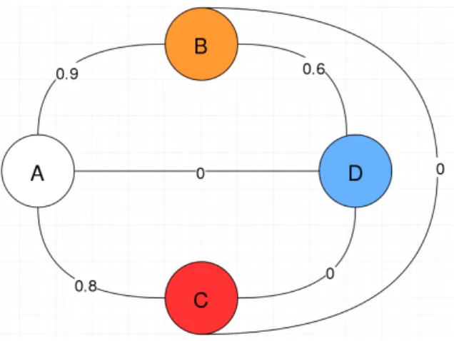
To illustrate this explanation, we may consider a very simple similarity graph (see figure 2.1).

Figure 2.1: A simple example to understand the role of Dii in the cost function.

In this example, we can find four individuals A, B, C and D and the similarities

between them. Each color represents a class, except white color, which indicates

that a node is unlabeled. In our case, A is the only unlabeled node and the rest of

them belong to different classes. The weights of the edges represent the similarities.

One could expect node A to be classified as belonging to the same class as B, since

it is the one with which shares the highest similarity. However, whenever the

pa-rameter µ in (2.1) is high enough to predict correctly all the labeled data, node A

is always classified in node C’s class. This is because C is more influential than B, since the sum of the similarities ofCwith the other nodes is only 0.8, whileB’s is 1.5.

Local and Global Consistency and regression

So far, we have commented on the functioning of the algorithm when it acts as a classifier, but our problem will be regression. So the natural question is whether it

will still work as a regressor and how it should be modified for that purpose. Lety

be the vector of ground truth labels, where unlabeled instances are labeled as 0, and

f the predicted labels. Then equation (2.1) would become

q(f) = N X i,j=1 Sij fi √ Dii − _pfj Djj !2 +µ N X i=1 (fi −yi)2. (2.2)

Here, we face two problems, which did not exist with classification. The simplest one is due to the label fitness term,PN

i=1(fi−yi)

2_{. If an unlabeled instance}_i _{is labeled}

(19)

2.1. SEMI-SUPERVISED ALGORITHMS 19 really small numbers. In the case of classification this did not happen or, being more

precise, this happened, but it was irrelevant. Why? BecauseFwas a matrix and the

label of a samplei was the index of the highest element in fi, so the absolute values of fi were irrelevant. However, in regression, the predicted label of an instance i is exactlyfi, so having smaller values of fi when i is unlabeled than when it is labeled

becomes a problem. A way of solving this, which we will adopt, is by setting yi to

the mean of the labeled instances wheni is unlabeled.

The second problem regards the label smoothness, N X i,j=1 Sij fi √ Dii − _pfj Djj !2 ,

and lies on the terms Dii and Djj. Suppose, as before, that i and j are a labeled

and an unlabeled instance respectively and that Sij ' 1. If Dii is a large number,

then fi/

√

Dii will be low and, therefore, fj/

p

Djj and, consequently, fj will be low. A way of tackling this problem consists in normalizing the rows of the similarity

matrix S, i.e., dividing each row by its sum so that Dii = 1 for each i. However,

this means that the resulting matrix Snorm could not be symmetric and, thus, the

algorithm cannot be applied. To satisfy the requirement of symmetry, we compute the following operation:

Snorm+STnorm

2 ,

and use this similarity matrix instead ofS, whose row sums are roughly 1.

Although these two drawbacks could make the algorithm not suit perfectly our prob-lem, it is interesting having this algorithm as a starting point to compare its perfor-mance with the more sophisticated versions of label propagation explained below.

2.1.3

Flexible Manifold Embedding

Similarly to LGC, Flexible Manifold Embedding (FME) [14] estimates the labelsF

by minimizing the following cost function:

g(F,W,b) = tr(FTLF)+βtr[(F−Y)TU(F−Y)]+µ(||W||2₊_γ_||_XT_W₊_1bT₋_F_||2₎_,

(2.3)

where U is an indicator matrix, that is a diagonal matrix, with its first l diagonal

elements, corresponding to labeled instances, equal to 1, while the last u diagonal

elements, corresponding to unlabeled instances, are equal to 0. W and b determine

the unknown linear regressor which maps the original samples to the label space. As with LGC, a closed-form solution, which is the one we will be using, can be found by setting the derivatives ofg with respect toW, b and Fas 0 (for more details on how to obtain it, see [14]). The solution would be

b= 1

l+u F

T

1−WTX1

(20)

20 CHAPTER 2. LEARNING ALGORITHMS F=β(βU+L+µγHc−µγ2Q)−1UY,

with Q=XT

cXc(γXTcXc+I)−1 and Hc=I−(1/(l+u))11T.

Flexible Manifold Embedding and regression

As with LGC, this algorithm was originally designed for classification tasks. Nonethe-less, it can easily be adapted to work as a regressor. Iff and yare real-valued vectors representing the predicted labels and the ground-truth labels, the cost function be-comes

g(f,w, b) =fTLf +β(f −y)TU(f −y) +µ(||w||2₊_γ_||_XT_w₊₁_b₋_f_||2₎_. _(2.4)

The first term controls the label smoothness, the second one the label fitness and the last term fits a linear regression between features and labels, where ||w||2 _is

a regularaztion term controlling the complexity of the model (thus, avoiding over-fitting). β,µandγare the parameters controlling the trade-off between all the terms. In spite of having been analysed in the case of LGC, the first two terms deserve further comment, since they present certain variations with respect to the previous algorithm. If we develope the expressionfT_Lf_{, it would be}

n

X

i,j=1

Sij(fi−fj)2.

This is the same as in LGC if we remove the terms Dii and Djj. So, as explained

before, this term is responsible of making similar images have similar labels. The second term, the label fitness, (f −y)T_U₍_f ₋_y_{) would be}

l

X

i=1

(fi−yi)2, whereas in the case of LGC it was

N

X

i=1

(fi−yi)2.

So the two problems that arised in the adaptation of LGC to regression vanish in the

case of FME. The first of them is solved by considering the indicator matrix U, so

that the label fitness term forgets about unlabeled data. The second problem, which was derived from the termsDii in the cost function, also does not occur, because the label smoothness term considered is much simpler.

(21)

2.1. SEMI-SUPERVISED ALGORITHMS 21

FME and unseen data

A really positive advantage of FME, which distinguishes it from many label propa-gation methods, e.g., from LGC, is its capacity of dealing with unseen data. Apart

from predicting the labels of the unlabeled data in vector f, it can predict unseen

data using the regression term in 2.4. Given the features of the unseen dataXunseen, its scores would be:

funseen =XTunseenw+1b.

Relationship between LGC and FME

The cost function of LGC in 2.1 can be expressed similarly to the cost function of FME in 2.3:

q(F) = tr(FTLFˆ ) +µtr[(F−Y)T(F−Y)].

2.1.4

Kernel Flexible Manifold Embedding

Kernel Flexible Manifold Embedding (KFME) [5] is the kernel version of FME and it was proposed to cope with highly non-linear data (when a linear regression has a poor performance). The cost function in this case is

g(F,V) = tr(FTLF)+βtr[(F−Y)TU(F−Y)]+αtr(VTKV)+λtr[(KV−F)T(KV−F)],

whereK is the kernel matrix of the data X, in which each element Kij is the result

of applying the kernel function to samples i and j. In our case, the kernel will be

Gaussian. This means that

Kij =e

−||xi −xj||

2

2t0σ2 _,

where σ2 _{is a measure of the variability of the data or, more concretely, it is the}

mean of the squares of the distances between all pairs of samples. t0 is the kernel

parameter, which will take different values.

A closed-form solution can be found again by setting the derivatives ofg with respect toF and V as 0 (for more details, see [14]). The solution is

V =AF

F=β[βU+L+αATKA+λ(KA−I)T(KA−I)]−1UY,

whereA =λ/α(I+λ/αK)−1_.

Kernel Flexible Manifold Embedding for regression

The cost function can also be defined for vectors of continuous real-valued labels f and yas follows:

(22)

22 CHAPTER 2. LEARNING ALGORITHMS

The interpretation is analogous to FME. The label smoothnes and label fitness crite-ria are exactly the same, while the linear regression becomes a non-linear regression thanks to the kernel trick. So the term (Kv−f)T₍_Kv₋_f_{) controls the loss in the}

non-linear regression and vTKv controls the complexity of the model.

KFME and unseen data

Similarly to FME, in KFME one can easily handle unseen data using the regression term in 2.5. To do so, given a set of unseen samplesxunseen

i |mi=1, one has to build the

kernel matrix of the unseen samplesKunseen ∈_Rm×N_{, where the element (}_{i, j}_{) is the} kernel function of the unseen samplei, xunseen

i , and the training samplej, xj. Then,

the predicted labels would be

funseen =Kunseenv.

2.1.5

Flexible Graph-based Semi-supervised Manifold

Em-bedding

Given the data matrix X, this algorithm [3] obtains a non-linear embedding by

optimizing a cost function based on several criteria, very similarly to the methods we have already seen in this chapter. The main difference is that up to the moment we

were obtaining a vector of predictions f or a matrix of classesF and now we have a

feature matrix Z ∈_RN×N_{. The objective of this algorithm is to clusterize the data} so that samples belonging to the same classes form a group and samples belonging to different classes are widely separated. However, since the cost function is not trivial at all, our starting point will be a very simplified case, where the learning is supervised andZ “lives” in RN×1 _{or, in other words, the projected data points have}

only one dimension. Therefore, in the next section we will be assuming that all the

N samples are labeled.

Supervised case with a single dimension

We will start defining the margin of a sample i. This is the difference between the

mean of the inter-class distances, which measure the distance between sample i and

samples belonging to different classes, and the mean of the intra-class distances, which

measure the distance between sample i and samples belonging to its same class. In

order to clusterize the data as has been commented, it is desirable for margins to be as large as possible. Assuming the number of dimensions of the non-linear embedding is 1, or equivalently that the non-linear projectionzis a vector in _RN (below we will generalize this toN dimensions), the margin of a sample ibelonging to a class Ck is mathematically defined as m(i) = 1 l−lk X j /∈Ck (zi−zj)2− 1 lk X t∈Ck (zi−zt)2, wherelk is the number of samples belonging to class Ck.

(23)

2.1. SEMI-SUPERVISED ALGORITHMS 23 The first term corresponds to the inter-class distance and the second one to the intra-class distance. However, since we wish to consider all of the samples and not just a

single one, we should maximize the mean margin of all of the samplesm.

m = 1 l l X i=1 m(i). (2.6)

We will now consider the weighted inter-class and the intra-class graphsGw and Gb, where nodes are all the samples. The former will be an undirected graph in which and edge will exist between two nodes if and only if they belong to the same class, while the second one will be directed and each edge starting at a nodeiwill end in a nodej belonging to a different class. The weight matrices associated to these graphs will be S_ijw =      1 lk if i∈Ck and j ∈Ck 0 if i∈Ck and j /∈Ck S_ijb =      0 if i∈Ck and j ∈Ck 1 l−lk if i∈Ck and j /∈Ck

After some algebraic manipulation (for further detail see [3]), one can express m in

equation 2.6 in terms of Sw _and _Sb_:

m= 2 lz T_D lz− 1 lz T_M lz,

whereDl =I+Db (Db is the diagonal matrix whose diagonal elements are the row

sums of Sb) and Ml = 3I+Db+Sb+SbT −2Sw.

We would like to maximize the mean margin m. However, there is no solution to

this problem. Why does this happen? Reasoning by contradiction, if we assume z0

were a solution which maximizes the margin, that would mean 2

lz T 0Dlz0− 1 lz T 0Mlz0

is as large as possible. However, if we consider a proportional vector zλ =λz0 with

λ >1, then the margin associated to zλ would be 2 lz T λDlzλ− 1 lz T λMlzλ = 2 l(λz0) T Dl(λz0)− 1 l(λz0) T Ml(λz0) = λ2 2 lz T 0Dlz0− 1 lz T 0Mlz0 ,

which isλ2 times the margin associated toz0 and, hence, it is larger. Thus, we have

reached an absurd because we were assumingz0 had the largest margin.

This reasoning leads us to a clear conclusion: the search space is too vast to find only one solution and, in addition, z0 and zλ are equivalent representations of the data, since they are proportional, so we should really get rid of the repeated solutions. A way of restricting the search space and avoiding this problem consists in imposing

zTDlz= 1.

Then, our maximization problem becomes a minimization one with an associated restriction:

z= arg min

z z

T

(24)

24 CHAPTER 2. LEARNING ALGORITHMS

Generalization to N dimensions

To generalize the problem above, the first step is to use more dimensions instead of only 1 and making use of the unlabeled data, which will be done as with the previous methods, using the label smoothness criterion. So the minimization problem has to take into account two criteria. Firstly, the label smoothness in various dimensions,

arg min

Z tr(Z

T_LZ₎_,

and, secondly, the maximization of the margin in a semi-supervised setting: arg min

Z tr(Z

T_M_˜

lZ) s.t. ZTD˜lZ=I.

In this context, ˜Ml ∈RN×N and ˜Dl ∈RN×N are the augmented forms of Ml ∈Rl×l and Dl ∈_Rl×l_{, that is} ˜ Ml = Ml 0 0 0 and D˜l = Dl 0 0 0 .

The zeros are due to the fact that there is no margin to be calculated for unlabeled samples. In addition, a regression term is added to the cost function, so that the

non-linear projection Z is as close as possible to a linear embedding. This permits

treating unseen samples, like in FME or KFME, by mapping them to the linear embedding. Considering all these factors the cost function becomes

e(Z,W,b) = tr(ZTLZ) +λtr(ZTM˜lZ) +µ(||W||2+γ||XTW+1bT −Z||2) s.t. ZTDlZ˜ =I.

||W||2 _{is, again, a regularization term controlling the overfitting. The solution can}

be found by generalized eigenvalue decomposition.

2.1.6

Similarity graphs

Considering that the key to learning from unlabeled data is the similarity between samples, observing how the choice of the similarity matrix affects the results seems to be important. For this sake, we have tried three types of similarity matrices based on feature and score similarities between samples. It is important to recall that a similarity is a value ranging from 0 (when samples are unalike) to 1 (when they are alike).

Feature similarities

Given two instances i and j, let xi and xj be their respective features. Then, two different similarities are considered. Firstly, the Gaussian similarity is given by

sgauss_ij =e−

||xi−xj||2

(25)

2.1. SEMI-SUPERVISED ALGORITHMS 25 were σ2 _{is the mean of} _||_x

i −xj||2 for i, j = 1,· · · , n. According to the formula,

samples are considered to be similar when their features are close in the Euclidean distance.

Secondly, the cosine similarity is defined as follows:

scos_ij =

xixj

||xi||||xj||

+ 1

2 .

This similarity corresponds to the cosine between vectorsxi and xj, rescaled so that it lies on the interval [0, 1], instead of [-1, 1]. So two samples are considered to be more similar when the angle formed by their respective vectors becomes narrower. The rescaling to avoid negative similarities is not strictly necessary for all the algo-rithms. In fact, it is only needed with LGC, because equation 2.1 uses the square roots of the row sums of the similarity matrix, √Dii, so these sums cannot be nega-tive. However, for simplicity, the rescaled cosine similarity is always used.

It is interesting to consider both similarities, since they measure different things. Even if using hundreds of dimensions makes the geometric sense vanish, how both similarities differ can be easily noticed, since the cosine similarity does not care about the norm of the features, while vectors with very different norm values will always be considered unalike by the Euclidean or Gaussian similarity.

Score similarity

Given two labeled samplesi andj, and their respective labelsyi and yj, they will be similar if the difference between the scores does not exceed a certain thresholdδ > 0. Mathematically this can be stated as

sscore_ij =    1 if |yi−yj|< δ 0 otherwise

This binary similarity is the simplest one which could have been considered and, even though it will not be studied here, it could be good idea to analyse more complex score similarities.

Construction of the similarity matrix

Three different types of similarity matrices are built in this study: the similarity matrix based only on Gaussian feature similarity and matrices which are based on Gaussian or cosine similarity and score similarity. All of them will depend on the idea of the k nearest neighbors.

The process is the following:

(26)

26 CHAPTER 2. LEARNING ALGORITHMS 2. For each of the samples theknearest neighbors are considered (k= 10 through-out all the work), while the farthest samples are considered to have 0 similarity. This can be understood as a directed graph where each node is a sample and the weight of each edge is the similarity between samples. The edges corre-sponding to the farthest neighbors are removed. An initial similarity matrix Sinitial is built based on the directed graph.

3. Since the similarity matrix has to be symmetric, a new similarity matrix S is

built according to the operation:

Sij = max(Sijinitial, S initial ji ),

which is the same as converting our directed graph into an undirected one by considering all the edges bidirectional instead of unidirectional.

When a feature similarity and the score similarity are considered, there is an

addi-tional step between step 1 and step 2. Before selecting the k nearest neighbors, all

the pairs whose score difference exceeds a given threshold δ are removed. Then, in

step 2, for each sample, the k nearest neighbors are selected among the remaining

samples (whose score difference is smaller than δ).

2.2

Supervised algorithms

In this section, three classical regression algorithms are presented, which will be com-pared with the semi-supervised algorithms in the next chapter to check whether the semi-supervised approach provides an improvement.

2.2.1

Mathematical notation of the supervised algorithms

The difference between the semi-supervised algorithms and the supervised algorithms is that the latter do not use the unlabeled data in training. This affects the notation, where we will have a clear separation between the training data and the test data. N

will be the number of training data andM the number of test data. Xtrain ∈RN×D and ytrain ∈ RN will note the training data matrix, where samples are represented as columns, and the labels of the training data, respectively. And the test data and labels will beXtest ∈RD×M and ytest ∈RM.

2.2.2

1-Nearest Neighbor

k-nearest neighbors (KNN) is a lazy learning algorithm, which means that it does

not have a real training phase, since it simply memorizes the training data. On the other hand, the prediction step is when the algorithm is actually working. In order to evaluate a new point, it finds the k nearest training points and the label assigned to this new point only depends on the labels of thek nearest neighbors. In our case,

(27)

2.2. SUPERVISED ALGORITHMS 27 will just find its nearest neighbor and copy its label.

This algorithm is fundamentally based on the concept of nearness; however, this can be relative, depending on the type of distance considered. In this work, three basic distances are used: the Euclidean distance, the Minkowski distance and the cosine distance. Given two real row vectors of sizen,x= [x1,· · · , xn] and y= [y1,· · · , yn], each of the distances is defined as follows:

• Euclidean distance:

d(x,y) =p(x−y)(x−y)T_.

• Minkowski distance of exponent p∈_N:

d(x,y) = n X i=1 |xi−yi|p !1/p .

The Euclidean distance is a particular case of the Minkowski distance, when

p= 2. • Cosine distance: d(x,y) = 1− xy T p (xxT₎₍_yyT₎.

The cosine distance derives from the cosine similarity and it ranges from 0 (when x= λy with λ > 0) to 2 (when x= λy with λ < 0). It is 1 when the

vectors pointing from the origin of the coordinate system to the points x and

y respectively are orthogonal. So this distance grows with the angle between

the vectors x and y.

2.2.3

Ridge Regression

Ridge regression (RR), named by Hoerl and Kennard [8], is a sophistication of the least squares method by adding a regularization term. It aims at minimizing the cost function

e(w) =||wTXtrain−ytrain||+λ||w||2,

where Xtrain usually is the centered and scaled training data, that is, each column

has mean 0 and standard deviation 1. The term||w||2 _{controls the complexity of the}

model or, in other words, it avoids overfitting.

2.2.4

Support Vector Regression

-insensitive Suport Vector Regression (-SVR) [18, 20] is a regression algorithm in

which an instance i with a label yi is considered to be correctly predicted by the

(28)

28 CHAPTER 2. LEARNING ALGORITHMS linear or non-linear (using the kernel trick). Firstly we will describe the linear case. Given an instancex, we aim at obtaining a regression function f(x) of the form

f(x) = wTx+b, with w,x∈_RD

and b ∈_R.

Similarly to Ridge Regression, -SVR is posed as a minimization problem in which

two terms have to be taken into account. On one hand, the regression fitness (taking into account that predictions in the interval [yi −, yi +] have 0 error) and, on

the other, the complexity of the model given by ||w||2_{. These conditions can be}

comprised in an optimization problem stated as follows:

min1 2||w|| 2 subject to yi−(wTxi+b)≤ wT_x i+b−yi ≤

The cost function corresponds to the complexity of the model and the two restrictions force the samples to be predicted correctly. This statement of the problem, though, is too rigid, since it does not permit any of the training samples to be predicted outside the tube. This can be tackled by adding slack variables ξi and ξi∗ permitting some deviations in the model:

min1 2||w|| 2₊_C l X i=1 (ξi+ξ∗i) subject to    yi−(wTxi+b)≤+ξi wTxi+b−yi ≤+ξ∗i ξi, ξi∗ ≥0 (2.7)

C is the constant which controls the trade-off between the complexity and the

flex-ibility of the model. A high C implies that ξi and ξi∗ tend to be lower, leading to a rigid model, where every sample has to be accurately classified and, in addition

||w||2 _{is not hardly penalized. Therefore, the model tends to overfitting. A low} _C

means just the opposite, tending the model to underfitting. So a correct choice of the

parameterC is a vital decision in order to get a good performance of the algorithm.

In figure 2.2 one can see how the regression error of-SVR, ζ, is computed, which is always lower than the real regression error, because predictions are considered to be correct within the given tolerance . So a real regression error of costs 0 and, for higher errors,ζ is obtained by substracting a quantity of to the real error.

Kernel Support Vector Regression

Kernel Support Vector Regression arises to overcome the limitations of the linear re-gression. Instead of considering the raw features of a samplex, a non-linear mapping of the features φ(x), is used before performing the linear regression. Equation 2.7

(29)

2.2. SUPERVISED ALGORITHMS 29

Figure 2.2: The soft margin loss, as shown in [19].

would be expressed as min1 2||w|| 2₊_C l X i=1 (ξi+ξi∗) subject to    yi−(wTφ(xi) +b)≤+ξi wTφ(xi) +b−yi ≤+ξi∗ ξi, ξ∗i ≥0

The solution can be found thanks to the dual optimization problem, where the use

of an explicit non-linear mapping φ is avoided and, instead, a kernel function K

implicitly maps the data non-linearly. Since this algorithm is not the main point of the work, we will skip the technical explanation regarding this part. So, for further detail, the reader can see the references [18, 20].

(30)

(31)

Chapter 3

Empirical study

3.1

General methodology

As mentioned in section 1.3.1, two datasets are used in our study: SCUT-FBP and

M2_{B. Most of the experiments have been carried out in SCUT-FBP, since it contains}

higher quality photos and, supposedly, it should make the learning easier. Labels in

SCUT-FBP lie on the interval (1, 5), whereas in M2_{B they lie on [1, 10]. In both}

cases, labels are scaled so that they lie on [0.1, 1], dividing by 5 in the first case and by 10 in the second.

Several of the algorithms used in this study have a number of parameters to be fixed. In all of these cases a grid search is conducted, that is, given a finite set of possible values for each parameter, all of the combinations are tried and the one giving the best error is selected.

All the matlab code used in these experiments is replicable downloading it from the

following link: https://github.com/AnneED/aesthetic-analysis.git.

3.1.1

Face features

Recent studies have proved that extracting features using a pretrained Convolutional Neural Network (CNN) can provide more than satisfactory results in computer vi-sion [17], often improving methods using other types of features and even if they are used in a task which is not exactly the one the network was trained to accomplish. Therefore, we are adopting this approach for our study, using the VGG-face network [15], which was trained for face identification and is available for matlab1_{. Figure 3.1}

shows its architecture.

The features are extracted from layer 7, right before the last fully-connected layer (fc8 in the diagram). Before propagating an image through VGG-face, it must be resized and the average of the network has to be substracted.

After extracting the features using the CNN, they are organized in a matrix, where each column represents the 4096 features of an image. The matrix is normalized using

1_{The network can be downloaded from}

http://www.vlfeat.org/matconvnet/pretrained/.

(32)

32 CHAPTER 3. EMPIRICAL STUDY

Figure 3.1: Architecture of VGG-face from [15].

L2 normalization (each column is divided by its Euclidean norm) and, then, the ma-trix is reduced from 4096 to 200 features using Principal Component Analysis (PCA).

3.1.2

Model evaluation

In order to have an idea of the effect of different data sizes during the training phase, which can be particularly interesting considering that we are working in a semi-supervised setting because there exist limited labeled data for this problem, many data size configurations are tested. In most of the experiments the labeled data con-stitute the 50%, the 70% or the 90% of all the data. On the other hand, when using semi-supervised algorithms the rest of the data is the unlabeled part, which is used in the training, as well as in the test phase, except for the experiment shown in table 3.10, in which the effect of testing in unseen data is studied.

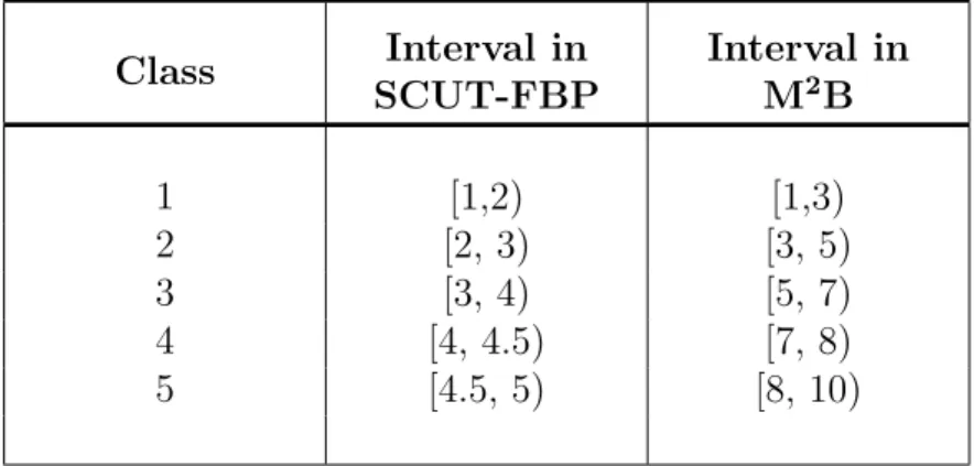
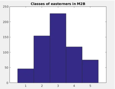
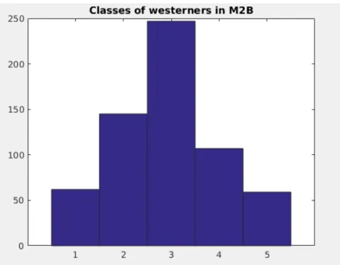
To have a good estimation of the error of the models, given the training/test percent-ages, each model is trained 10 times with 10 different splits of the data, sampled using stratification so that the label distributions are roughly equal in both the training and the test sets. The error is estimated as the mean of the errors of the 10 splits. Since our labels are continuous numbers, five “artificial” classes are created to carry out the stratification easily, as shown in table 3.1. In figures 3.2, 3.3 and 3.4 his-tograms of the classes are presented. These procedures will be maintained in each of the experiments unless otherwise indicated. Each model is evaluated using the performance metrics described in the next section.

3.2

Performance metrics

In order to measure the performance of the different algorithms, four metrics are taken into account: the mean absolute error (MAE), the root mean square error

(33)

3.2. PERFORMANCE METRICS 33 Class Interval in SCUT-FBP Interval in M2_B 1 [1,2) [1,3) 2 [2, 3) [3, 5) 3 [3, 4) [5, 7) 4 [4, 4.5) [7, 8) 5 [4.5, 5) [8, 10)

Table 3.1: Transformation of the labels from real numbers to discrete classes.

Figure 3.2: Histogram of classes in SCUT-FBP dataset.

Mean absolute error

Lety1, y2,· · · , yn be the ground truth labels and f1, f2,· · · , fn the estimated labels,

then the mean absolute error of the prediction is given by:

M AE = 1 n n X i=1 |yi−fi|.

Root mean square error

Let y1, y2,· · · , yn be the ground truth labels and f1, f2,· · ·fn the estimated labels,

then the root mean square error of the prediction is given by:

RM SE = v u u t 1 n n X i=1 (yi−fi)2.

(34)

34 CHAPTER 3. EMPIRICAL STUDY

Figure 3.3: Histogram of the classes of the easterners in M2B dataset.

Pearson correlation coefficient

Let y1, y2,· · · , yn be the ground truth labels and f1, f2,· · ·fn the estimated labels,

then the Pearson’s correlation coefficient measures the linear correlation between the ground truth and the estimated labels and is given by:

P C = Pn i=1(yi−y¯)(fi−f¯) pPn i=1(yi −y¯) q Pn i=1(fi−f¯) ,

where ¯f and ¯y are the means of the estimated labels and the ground truth labels

respectively.

The P C is a number in the interval [-1, 1]. It measures to what extent the points

(yi, fi), withi= 1,· · · , n, fit in their regression line. AP C around 1 or -1 means that there is a high linear correlation, where the slope of the regression line is positive, if

the PC is 1, or negative, if the PC is -1. On the other hand, a P C around 0 means

that there exists no linear correlation.

In our particular case, a PC as close to 1 as possible is desirable, since a perfect prediction would be one in which fi =yi, in other words, the pairs (yi, fi) lie on the line y=x.

(35)

3.2. PERFORMANCE METRICS 35

Figure 3.4: Histogram of the classes of the westerners in M2B dataset.

-error

Lety1, y2,· · · , yn be the ground truth labels and f1, f2,· · · , fn the estimated labels,

then the -error of the prediction is given by:

-error = 1 n n X i=1   1−e −(yi−fi) 2 2σ2 i   ,

whereσi is the standard deviation of the ratings of all the raters of image i.

This error lies on the interval [0,1). Unlike the MAE and the RMSE, - error takes

into account the ratings of all the raters of each image. Since beauty is a relative concept, raters may not agree when judging it. What is more, one can consider two types of faces: the ones which are found attractive by certain people and which are not by others and the faces which are judged mostly equally by all the raters. In other words, the ratings of the different raters of a face of the first group will have a higher standard deviation than the ratings of a face of the second group. So, if the predictor does not exactly predict the mean of the ratings of a face with a high standard deviation, the error is considered not to be so relevant, since there is no human agreement about the rating of that particular face. This is why in the formula the square difference between the real score and the estimated score (yi−fi)2 is divided by σ2

(36)

36 CHAPTER 3. EMPIRICAL STUDY

3.3

Results on SCUT-FBP dataset

3.3.1

The baseline

Table 3.2 shows the performance of an algorithm which, regardless of the face which it is presented, the score returned by it will be the average of the labels of the training images. This will be our starting point. While the PC could not be worse, the mean average error is not so high, since the labels follow a normal distribution and most of the images are gathered around the average.

3.3.2

Local and Global Consistency

As explained in section 2.1.2, LGC has a parameterµwhich has to be adjusted. In all the experiments related to LGC, its value is selected among the following so that the MAE is minimized: {10−6,10−5,10−4,10−3,10−2,10−1,1,10,102,103,104,105,106}. As hypothesized in the previous chapter in section 2.1.2, the “label” given to

unla-beled images, that is, the value of yi when i corresponds to an unlabeled instance,

seems to affect the performance of this algorithm when it comes down to regression. Table 3.3 confirms this assumption. It shows the performance of the algorithm when unlabeled instances are “labeled” as 0 or as the mean of the labeled instances. The similarity matrix used to compute the Laplacian is the simplest one, based only on Gaussian feature similarity. Being the difference so considerable, we are setting yi

(when i corresponds to an unlabeled instance) as the average in the rest of the

ex-periments regarding LGC.

Table 3.4 shows the results of applying LGC with different training/test sizes and

Laplacians (where δ = 0.1, when computing the similarity matrices) and table 3.5

shows the effect of similarity graph normalization in LGC when the Laplacian is only based on feature similarity. Even though the improvement is apparent, which was forseeable considering the discussion in section 2.1.2, it is not as marked as could be expected.

3.3.3

Flexible Manifold Embedding

As mentioned in section 2.1.3, FME has three parameters,β, µ and γ to be adjusted.

All of them are selected among{10−9,10−6,10−3,1,103,106,109}in order to optimize the MAE.

Table 3.6 shows the performance of FME considering different data sizes and Lapla-cians (whereδ = 0.1, when computing the similarity matrices), proving that, in this case, the results are independent of the Laplacian.

3.3.4

Kernel Flexible Manifold Embedding

As mentioned in section 2.1.4, KFME has three parameters to be adjusted in its

(37)

3.3. RESULTS ON SCUT-FBP DATASET 37 width of the kernel function. β is selected among {0.1,1,10,100,1000,10000}, α

among {0.0001,0.001,0.01,0.1,1,10}, λ among {1,10,50,100,1000} and t0 among

{1/8,1/4,1/2,1,2,4,8}.

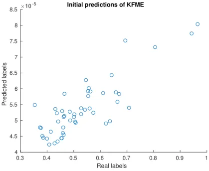
Unexpectedly, being KFME the kernelized version of FME, the first time KFME was used in this study, the MAE was worse than using the simpler algorithm. More surprisingly, when the PC was optimized in KFME, it was around 0.85, slightly out-performing FME. Given this information, we should remember that the PC measures the linear correlation between two variables or, in other words, how well a regression line between these two variables would fit. A perfect performance would be one in which, for each test sample i, the predicted label is exactly the real label, that is

yi =fi, so the MAE would be 0 and the PC 1, because, if we plot each pair (fi, yi),

it lies on the line y = x. However, having a poor MAE and such a good PC means

that the pairs (fi, yi) almost lie on a perfect line, but since it cannot bey =x, it has to be a distorted liney=ax+b. In fact, after plotting this in our specific problem, the result was the corresponding to figure 3.5.

0.3 0.4 0.5 0.6 0.7 0.8 0.9 1 Real labels 4 4.5 5 5.5 6 6.5 7 7.5 8 8.5 Predicted labels

10-5 Initial predictions of KFME

Figure 3.5: Initial predictions of KFME.

The way of fixing this problem was just rescaling the output f of the algorithm,

according to the formula:

fscaled = min(ytrain) + (f −min(ytrain))

max(ytrain)−min(ytrain)

max(f)−min(f) . (3.1)

Table 3.7 shows the improvement when scaling the output of the algorithm f. The

possible reasons of this need to scale f will be discussed in section 4.1. In addition, after observing the great difference of scaling the output in KFME, the scaling was also used in FME, but no improvement was observed in this case.

Table 3.8 shows the performance of KFME using different training/test proportions

(38)

38 CHAPTER 3. EMPIRICAL STUDY similarity matrices). It seems that using score similarity as well as feature similar-ity slightly improves the performance, but the difference is not so marked. On the

other hand, table 3.9 shows the results of varying the value of δ when computing

the Laplacian based on Gaussian feature similarity combined with score similarity.

Although the optimal value seems to be around 0.2, the value of δ does not seem to

affect strongly the results.

An experiment on unseen data

It could be argued that our study, as yet, has a major flaw, namely, that the unlabeled data is used both in training and in testing and, therefore, that nobody can ensure its correct performance on new data. This experiment is an attempt to address the unseen data case. We are considering the following partition of the data (sampled with stratification): 200 images will form the labeled data, 200 will be the unlabeled data and the remaining 100 will be the test data. The algorithm will be trained on the 400 labeled and unlabeled instances (the 80% of the data) and it will be tested on the remaining 100 (the 20% of the data), as explained in section 2.1.4, using the linear regression on the kernel matrix associated to unseen samples.

Table 3.10 shows the best of the models considering all the possible combinations of parameters. In this case, only one data partition has been considered, instead of the usual 10 splits, in order to simplify the task. In addition, when scaling the images as described in equation 3.1, instead of taking the maximum and minimum labels of the labeled training data, since there are only 200 labeled instances, the maximum and the minimum of all the data are used.

This experiment shows that KFME can work correctly for unseen images.

3.3.5

Flexible Semi-supervised Embedding

As opposed to the other semi-supervised algorithms, which aim at classification or direct regression, here we will see the results of using the embedding described in section 2.1.5, combined with a supervised algorithm. Firstly, we will be using linear

-SVR and then 1-NN. The algorithm to obtain the embedded features, which we

will be naming “zwb features”, has three parameters, λ, µand γ, that have to be

adjusted. We are choosing all of them among {10−9_,₁₀−6_,₁₀−3_,₁_,₁₀3_,₁₀6_,₁₀9_}_{. In}

addition, the number of dimensions of the output Z used to represent the data has

to be selected, since, similarly to PCA, the matrixZ can be cropped so that the data has fewer dimensions. The possible number of dimensions will be ranging from 10 to 500, with a step of 10, and the parametert0 used in the kernel function, which is the

same as in KFME, has to be selected among{1/8,1/4,1/2,1,2,4,8}.

The training/test configuration in -SVR and in 1-NN will be the same as the

la-beled/unlabeled configuration when using the semi-supervised embedding.

In-SVR we will be adjusting the parametersC and . Since there are 6 or 7

(39)

3.3. RESULTS ON SCUT-FBP DATASET 39 using the kernel version, and 2 in-SVR) and this can be very time-consuming, firstly the parameters in the embedding are optimized using the default parameters for

SVR, and then the parameters in-SVR are optimized. C and are selected among

{5,7.5,10,12.5,15,17.5,20,22.5,25,27.5,30,32.5}and{0,0.005,0.01,0.02,0.03,0.04},

respectively, after seeing, using a wider search, that the optimal values were around

20 and 0.01. Table 3.11 shows the comparison of applying-SVR on the raw features

or on the ones obtained with the embedding. Judging by the results, it is not clear that using the non-linear transformation has a positive effect. However, there is a slight improvement for the 90%/10% partition and for the non-kernelized variant. Our future work is to integreate the score similarity in the margin used by the non-linear projection method.

Experiment on discrete classes

On the other hand, table 3.12 shows a clear improvement when using the non-linear transformation (if we look at the Euclidean distance), possibly implying that, even though this embedding works properly on discrete classes, maybe it is not so suitable for regression problems. In this second case, 3 discrete classes are created: most at-tractive, average beauty and least attractive. To create these classes only 400 images are used and the intermediate classes are discarded. In this case, only 1 split of the data has been considered, instead of repeating the experiment 10 times. Table 3.13 shows the normalized score intervals on which lie each of the classes.

Table 3.12 shows the correct prediction rates of class 1, class 2, class 3 and all of the samples. When zwb features are used, the parameters are optimized in order to obtain the best total correct prediction rate. When using the Euclidean distance, the improvement in the prediction is remarkable, whereas the cosine distance does not imply a real improvement. However, this has much sense. The graph-based embed-ding method aims at clusterizing the samples depenembed-ding on their classes and, for this purpose, it uses the Euclidean distance, so this is the reason for the 1-NN Euclidean classifier to work better.

3.3.6

Supervised algorithms

In this section, we will report the performances of three supervised algorithms,

namely, 1-Nearest Neighbor, Ridge Regression and -insensitive Support Vector

Re-gression, in order to compare them with the semi-supervised case.

Table 3.14 shows the results of 1-NN on the raw features of SCUT-FBP with the Eu-clidean distance, the cosine distance and the Minkowski distance with the exponent

p= 1. The best results are achieved by the Euclidean distance with a training/test

configuration of 90%/10%.

Table 3.15 shows the results of applying Ridge Regression on SCUT-FBP dataset.

As explained in section 2.2.3, Ridge Regression has a parameter µ that has to be

(40)

40 CHAPTER 3. EMPIRICAL STUDY 0.1, 1, 10, 50, 100, 250, 500, 1000, 5000, 10000}.

Table 3.16 shows the results of applying-insensitive SVR with a linear and a

Gaus-sian kernel. In the first case, two parameters have to be adjusted, C and , which

have been selected among {0.00001, 0.0001, 0.001, 0.01, 0.1, 0.2, 0.3, 0.4, 0.5, 0.6, 0.7, 0.8, 0.9, 1, 2, 3, 4, 5, 10, 20, 3}and{0, 0.001, 0.0025, 0.005, 0.01, 0.02, 0.03, 0.04, 0.05, 0.06, 0.07, 0.08, 0.09, 0.1, 0.15}. In the second case there is an additional kernel parameter, which has been chosen among{1/25,1/24,1/8,1/4,1/2,1,2,4,8,24,25}.

3.3.7

Method comparison: Regression Error Characteristic

curve

A way of plotting and comparing a number of regression methods is using the Re-gression Error Characteristic (REC) curve [2]. Given a reRe-gression method and a test sampleilabeled asyi and predicted as fi, the regression error of this test sample can be either its squared error, (yi−fi)2, or its absolute error,|yi−fi|. We will be using

the latter. We can fix a tolerance value and count the number of images whose

error is smaller than the tolerance. This is exactly what the REC curve plots. The

X axis will be a range of tolerances and the Y axis will be the proportion of images whose error is smaller than this tolerance.

0 0.05 0.1 0.15 0.2 0.25 0.3 Tolerance 0 0.1 0.2 0.3 0.4 0.5 0.6 0.7 0.8 0.9 1 Proportion of images REC curves Baseline NN RR SVR LGC FME KFME

Figure 3.6: REC curves of different methods. The steeper a curve is the better is the performance of the algorithm.

Figure 3.6 shows the REC curve of the best models of the mean predictor, 1-NN,

(41)

3.4. RESULTS ON M2B DATASET 41 the data constitute the labeled part. A steep curve indicates that a greater number of images has smaller errors and the area over the curve is an estimate of the error. Hence, a smaller area indicates a better performance.

Having a quick look at the figure, it seems clear that KFME (in dark blue) outper-forms all the others. For a more detailed comparison, see table 3.17, which summa-rizes the best results obtained by each algorithm with a fixed data configuration of 90%/10%.

3.4

Results on M

2

B dataset

In this section, we will see the results on M2_{B dataset, with a configuration of 50% of}

the samples as labeled data and the other 50% of the samples as the unlabeled/test data. As stated in the beginning of the chapter, all the experiments are carried out doing 10 stratified splits of the data, except for table 3.23.

3.4.1

The baseline

Table 3.18 shows the results of an algorithm which returns always the average of the labels of the training images, regardless of the image which it is presented. The MAE and the RMSE are much higher than the baseline in SCUT-FBP (table 3.2). This is due to two facts: firstly, the normalized labels lie on a narrower interval in

SCUT-FBP (the lowest label in SCUT-FBP is 0.2394, while on M2B it is 0.1). In

addition, even though in both datasets the beauty scores roughly follow a Gaussian

distribution, in SCUT-FBP this is much sharper, implying that labels in M2_{B do not}

gather as much around the mean.

3.4.2

Local and Global Consistency

Table 3.19 in M2_{B is the equivalent to table 3.4 in SCUT-FBP, with the only}

differ-ence that in this case the similarity matrix has been normalized after seeing that the results in SCUT-FBP improved thanks to normalization (table 3.5).

3.4.3

Flexible Manifold Embedding

Table 3.20 represents the results of using FME on M2_{B under the same conditions}

as in 3.6. The results are independent of the type of similarity used to build the Laplacian matrix.

3.4.4

Kernel Flexible Manifold Embedding

Tables 3.21 and 3.22 are the corresponding to tables 3.8 and 3.9 in SCUT-FBP. It is not clear which type of similarity graph is the most convenient. In this case, the choice ofδin the similarity graph construction does not truely affect the results (the

(42)

42 CHAPTER 3. EMPIRICAL STUDY slight difference is only appreciated in the last decimal of the PC).

3.4.5

Flexible Semi-supervised Embedding

Tables 3.23 and 3.24 are the corresponding to tables 3.12 and 3.11 in SCUT-FBP. The three classes used in table 3.23 are described in table 3.25. In this experiment only the eastern samples have been taken into account. It seems that, contrary to what happened with SCUT-FBP, in both cases using the non-linear embedding im-proves the results.

(43)

3.5. TABLES 43

3.5

Tables

Data size MAE RMSE PC -error

50% train / 50% test 0.1009 0.1351 0.0000 0.2586

70% train / 30% test 0.0979 0.1322 0.0000 0.2479

90% train / 10% test 0.0987 0.1309 0.0000 0.2557

Table 3.2: Results of the baseline.

Data size Labels MAE RMSE PC -error

Zero 0.2711 0.3032 0.1002 0.7395 Mean 0.0940 0.1230 0.4520 0.2417 50% labeled 50% unlabeled Zero 0.1711 0.2137 0.0976 0.4388 Mean 0.0876 0.1144 0.5646 0.2212 70% labeled 30% unlabeled Zero 0.1100 0.1497 0.1153 0.2635 Mean 0.0850 0.1097 0.6223 0.2134 90% labeled 10% unlabeled

Table 3.3: Difference between settingyi as 0 or as the mean of the known labels when

(44)

44 CHAPTER 3. EMPIRICAL STUDY

Data size Laplacian MAE RMSE PC -error

Gaussian 0.0940 0.1230 0.4520 0.2417 Gaussian + score 0.0945 0.1211 0.4777 0.2481 Cosine + score 0.0946 0.1212 0.4755 0.2483 50% labeled 50% unlabeled Gaussian 0.0876 0.1144 0.5646 0.2212 Gaussian + score 0.0889 0.1115 0.5934 0.2340 Cosine + score 0.0889 0.1115 0.5917 0.2341 70% labeled 30% unlabeled Gaussian 0.0850 0.1097 0.6223 0.2134 Gaussian + score 0.0954 0.1144 0.6423 0.2686 Cosine + score 0.0953 0.1144 0.6417 0.2684 90% labeled 10% unlabeled

Table 3.4: Results of LGC using different Laplacians.

Data size Laplacian MAE RMSE PC -error

Raw 0.0940 0.1230 0.4520 0.2417 Normalized 0.0928 0.1217 0.5952 0.2375 50% labeled 50% unlabeled Raw 0.0876 0.1144 0.5646 0.2212 Normalized 0.0861 0.1132 0.6905 0.2169 70% labeled 30% unlabeled Raw 0.08