Receptive fields optimization in deep learning for enhanced interpretability, diversity, and resource efficiency.

(1)

University of Louisville

ThinkIR: The University of Louisville's Institutional Repository

Electronic Theses and Dissertations

5-2019

Receptive fields optimization in deep learning for

enhanced interpretability, diversity, and resource

efficiency.

Babajide Odunitan Ayinde

University of Louisville

Follow this and additional works at:https://ir.library.louisville.edu/etd

Part of theComputational Engineering Commons,Other Electrical and Computer Engineering

Commons, and theSignal Processing Commons

This Doctoral Dissertation is brought to you for free and open access by ThinkIR: The University of Louisville's Institutional Repository. It has been accepted for inclusion in Electronic Theses and Dissertations by an authorized administrator of ThinkIR: The University of Louisville's Institutional Repository. This title appears here courtesy of the author, who has retained all other copyrights. For more information, please contact

[email protected].

Recommended Citation

Ayinde, Babajide Odunitan, "Receptive fields optimization in deep learning for enhanced interpretability, diversity, and resource efficiency." (2019).Electronic Theses and Dissertations.Paper 3243.

(2)

RECEPTIVE FIELDS OPTIMIZATION IN DEEP LEARNING FOR ENHANCED INTERPRETABILITY, DIVERSITY, AND RESOURCE EFFICIENCY

By

Babajide Odunitan Ayinde

B.S., Obafemi Awolowo University, 2011

M.S., King Fahd University of Petroleum and Minerals, 2015

A Dissertation

Submitted to the Faculty of the

J.B. Speed School of Engineering of the University of Louisville in Partial Fulﬁllment of the Requirements

for the Degree of

Doctor of Philosophy in Electrical Engineering

Electrical and Computer Engineering University of Louisville

Louisville, Kentucky

(3)

(4)

Submitted by

Babajide Odunitan Ayinde

A Dissertation Approved on

January 23, 2019

by the Following Dissertation Committee:

Dr Jacek Zurada, Dissertation Director

Dr Tamer Inanc

Dr Eric Rouchka

(5)

DEDICATION

This is dedicated to God Almighty for availing the strength, inspiration, knowledge, and understanding required to successfully complete this dissertation. I also dedicate this work to my father Dr Folorunsho Ayinde and my late mother Felicia Mojisola Ayinde. To my beloved wife Ajoke Ayinde and son David Ayinde who have been affected in every way possible by this rigorous quest.

(6)

ACKNOWLEDGMENTS

I would like to express my profound gratitude to my advisor, Dr. Jacek Zu-rada, Director of the Computational Intelligence Laboratory at the University of Louisville, for his valuable contributions, guidance, and support towards the com-pletion of this work. I would also like to appreciate the School of Interdisciplinary and Graduate Studies, University of Louisville for awarding me the Dissertation Completion Fellowship to enable me put this work together. My appreciation also goes to Dr Tamer Inanc for the knowledge impacted through the Digital Signal Processing class and also for being one of my dissertation committee members. I would also like to thank Dr. Eric Rouchka and Dr. Huacheng Zeng for agreeing to serve on the dissertation committee. I am grateful for their suggestions, encour-agements, and advice.

There are a number of people without whom this dissertation might not have been written, and to whom I am greatly indebted. I thank my wife and son, Ajoke and David, for their patience, sacriﬁce, and constant support while this dis-sertation slowly assumes its current form. I am indebted to my dad Dr. Folorunsho Ayinde, my parents-in-law Mr and Mrs Chiazor Ndidi, and Mr and Mrs Bamidele Oresegun for their love, support, and words of encouragement. Thanks to all my siblings, Dr Olusola, Engr. Olugbenga, Mrs Olukemi Oyem, Mrs Omobola Favour, Engr. Ayokunle, Mrs Omolola Akinrinde, Engr. Tolulope for all their support and prayers. I am grateful to all my friends and colleagues at University of Louisville for the wonderful times we shared. A big thank you to everybody who contributed in one way or the other to the success of this dissertation. Ultimately, I thank Almighty God for every success in this process.

(7)

ABSTRACT

Babajide Odunitan Ayinde January 23, 2019

In both supervised and unsupervised learning settings, deep neural net-works (DNNs) are known to perform hierarchical and discriminative representa-tion of data. They are capable of automatically extracting excellent hierarchy of features from raw data without the need for manual feature engineering. Over the past few years, the general trend has been that DNNs have grown deeper and larger, amounting to huge number of final parameters and highly nonlinear cas-cade of features, thus improving the flexibility and accuracy of resulting models. In order to account for the scale, diversity and the difficulty of data DNNs learn from, the architectural complexity and the excessive number of weights are of-ten deliberately built in into their design. This flexibility and performance usu-ally come with high computational and memory demands both during training and inference. In addition, insight into the mappings DNN models perform and human ability to understand them still remain very limited. This dissertation ad-dresses some of these limitations by balancing three conflicting objectives: compu-tational/memory demands, interpretability, and accuracy.

This dissertation ﬁrst introduces some unsupervised feature learning meth-ods in a broader context of dictionary learning. It also sets the tone for deep

(8)

autoencoder learning and constraints for data representations in light of remov-ing some of the aforementioned bottlenecks such as the feature interpretability of deep learning models with nonnegativity constraints on receptive fields. In ad-dition, the two main classes of solution to the drawbacks associated with over-parameterization/over-complete representation in deep learning models are also presented. Subsequently, two novel methods, one for each solution class, are pre-sented to address the problems resulting from over-complete representation ex-hibited by most deep learning models. The first method is developed to achieve inference-cost-efficient models via elimination of redundant features with negligi-ble deterioration of prediction accuracy. This is important especially for deploying deep learning models into resource-limited portable devices. The second method aims at diversifying the features of DNNs in the learning phase to improve their performance without undermining their size and capacity. Lastly, feature diversi-fication is considered to stabilize adversarial learning and extensive experimental outcomes show that these methods have the potential of advancing the current state-of-the-art on different learning tasks and benchmark datasets.

(9)

TABLE OF CONTENTS

DEDICATION . . . iii

ACKNOWLEDGMENTS . . . iv

ABSTRACT . . . v

List of Tables . . . x

List of Figures . . . xii

CHAPTER INTRODUCTION . . . 1

I. CONSTRAINED FEATURE LEARNING . . . 4

A. Dictionary Learning via Sparse Coding . . . 4

B. Dictionary Learning via Nonnegative Matrix Factorization (NMF) 6 C. Dictionary Learning via Constrained Autoencoders . . . 7

1. Constrained Autoencoders for Sparse Representation . . . . 9

2. Constrained Autoencoders for Part-based Data Represen-tation . . . 11

II. CONSTRAINED AUTOENCODERS FOR ENHANCED DATA UN-DERSTANDING . . . 16

A. L1/L2-Nonnegativity Constrained Sparse Autoencoder (L1/L2 -NCSAE) . . . 17

1. Implication of imposing nonnegative parameters with com-posite decay function . . . 19

2. Experimental Results . . . 20

(10)

b. Unsupervised Semantic Feature Learning from Textual

Data . . . 29

c. Illustration of Understandable Feature Extraction byL1/L2 -NCSAE . . . 30

B. Deep Learning of Understandable Features using CascadedL1/L2 -NCSAE . . . 33

1. Image Classiﬁcation with Enhanced Interpretability . . . 35

2. Document Categorization with Enhanced Interpretability . 39 3. Performance Evaluation on Supervised Learning . . . 43

C. Conclusion . . . 45

III. UNSUPERVISED NONREDUNDANT FEATURE EXTRACTION . . . 46

A. Filtering Redundancy Elimination in Autoencoder-based Deep Networks . . . 47

1. Filter Clustering and Reduction . . . 48

a. Static Reduction of the Number of Redundant Filters . . 48

b. Dynamic Reduction and Reconciliation of Filters . . . . 50

B. Experimental Setup . . . 52

a. Unsupervised Feature Reduction via Filter Pruning . . . 61

b. Effect of Redundant Feature Pruning on Supervised Learn-ing . . . 64

IV. REDUNDANCY-BASED FILTER PRUNING IN DEEP CONVOLU-TIONAL NEURAL NETWORKS . . . 74

A. Convolutional Feature Clustering and Pruning . . . 78

1. Method A: Pruning of Redundant Filters . . . 80

2. Method B: Pruning of Randomn_f Filters . . . 82

(11)

1. VGG-16 on CIFAR-10 . . . 87

2. RESNET-56/110 on CIFAR-10 . . . 91

3. Prune and Train from Scratch . . . 101

V. FEATURE DIVERSIFICATION IN DEEP NEURAL NETWORKS . . . 103

A. Enhancing Feature Diversity by enforcing Dissimilar Feature Ex-traction . . . 106

1. Diversity Regularization . . . 108

2. Implications of imposing feature diversity . . . 110

B. Online Redundant Filter Detection and Dropout . . . 111

1. Online Filtering Redundancy Dropout . . . 112

2. Online Redundancy-based Dropout . . . 113

C. Experiments . . . 115

1. Feature Evolution during Training . . . 117

2. Diversity Regularized Image Classiﬁcation . . . 122

3. Diversity Regularized Natural Language Inference . . . 126

D. Diversity Regularized Adversarial Learning (DiReAL) . . . 131

E. Conclusion . . . 133

VI. CONCLUSIONS . . . 136

REFERENCES . . . 139

(12)

LIST OF TABLES

1 Classiﬁcation accuracy on MNIST and NORB dataset [1] . . . . 44

2 Parameter settings [2] . . . 54

3 Classiﬁcation performance on MNIST dataset using initial

net-work conﬁguration 784-200-20-10 [2]. . . 65

8 Classiﬁcation performance on NORB dataset [2]. . . 72

9 Pruning performance on CIFAR dataset using VGG-16 model

atτ =0.54 [3]. . . 92

10 Performance evaluation for three pruning techniques on

CIFAR-10 dataset. Performance with the lowest test error is reported [3]. 93

11 Performance evaluation of three pruning techniques for ResNet

56/110 trained on CIFAR-10 dataset. Performance with the lowest test error is reported [3]. . . 95

12 FLOP and CPU time reduction for inference. Operations in

convolutional and fully connected layer are considered for com-puting FLOP [3]. . . 101

(13)

13 Performance on CIFAR dataset [3]. . . 102

14 Test-train error gap on MNIST [4] . . . 120

15 Test error(%) on MNIST. Source: [4] . . . 122

16 Test error(%) on CIFAR-10 without data augmentation. Source:

[4] . . . 125

17 Validation error on ImageNet. Source: [4] . . . 126

18 A select examples from SNLI dataset where E, C, and N

repre-sent Entailment, Contradiction, and Neutral, respectively. Source: [4] . . . 128

(14)

LIST OF FIGURES

1 Illustration of Data Matrix Factorization (X ≈ ΦA). X is the

data matrix, columns ofΦare basis vectors, and columns ofA

are the encodings of the samples [5]. . . 5

2 Schematic diagram of a three-layer AE . . . 8

3 RFs or weights of randomly selected 32 out of 196 (n = 196)

hidden neurons of (a) NNSAE (b) NCAE trained using MNIST dataset. Black pixels indicate negative, grey pixels indicate zero-valued weights and white pixels indicate positive weights. The range of weights are scaled to [-1,1] and mapped to the

graycolor map.w=−1 is assigned to black,w =0 to grey, and

w=1 is assigned to white color [5]. . . 12

4 Representation of test image as a linear combination of 4 out of

196 constrained RFs and decoding ﬁlters learned from MNIST dataset using NCAE with linear output activation function.

In-put consist of 784 values corresponding to a 28×28 pixel

im-age. Only 70 RFs with largest activations to test image "6" and their corresponding decoding ﬁlters are shown. The RFs and the decoding ﬁlters are rescaled and portrayed as images on the right hand side. Black pixels indicate negative, and white pix-els indicate positive weights. The range of weights are scaled

to [-1,1] and mapped to the graycolor map.w=−1 is assigned

to black,w = 0 to grey, and w = 1 is assigned to white color.

(15)

5 Absolute function approximation using quadratic smoothing

functions withκ= 0.4, 0.7, 1.0 and 1.5 . . . 20

6 (a) Symmetric (G3) and skewed (G1 and G2) weight

distribu-tions. Decay function with three values ofα1andα2for weight

distribution (b)G3(c)G1and (d)G2. [1] . . . 21

7 196 receptive ﬁelds (W(1)) learned from MNIST digit data set

using (a) SAE, (b) DpAE (c) NCAE, and (d) L1/L2-NCSAE.

Black pixels indicate negative, and white pixels indicate pos-itive weights. The range of weights are scaled to [-1,1] and

mapped to the graycolor map. w = −1 is assigned to black,

w=0 to grey, andw=1 is assigned to white color [1]. . . 23

8 Encoding weights (W(1)) histograms learned from MNIST digit

data set using (a) SAE, (b) DpAE (c) NCAE, and (d) L₁/L₂

-NCSAE [1]. . . 24

9 (a) Reconstruction error and (b) Sparsity of hidden units

mea-sured by KL-divergence using MNIST train dataset with p =

0.05 [1]. . . 24

10 t-SNE projection [6] of 196D representations of MNIST

hand-written digits using (a) SAE (b) DpAE (c) NCAE (d) L₁/L2

-NCSAE [1]. . . 25

11 Weights of randomly selected 90 out of 200 receptive ﬁlters

of (a) SAE (b) DpAE (c) NCAE, and (d) L₁/L2-NCSAE using

NORB dataset. The range of weights are scaled to [-1,1] and

mapped to the graycolor map. w <= −1 is assigned to black,

(16)

12 The distribution of 200 encoding (W(1)) and decoding ﬁlters

(W(2)) weights learned from NORB dataset using (a) DpAE (b)

NCAE (c)L1/L2-NCSAE [1]. . . 27

13 Visualizing 20D representations of a subset of Reuters

Docu-ments data using (a) DpAE, (b) NCAE, and (c) L1/L2-NCSAE

[1]. . . 32

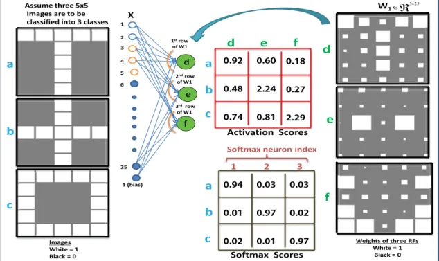
14 Illustration of constrained (non-negative) RF feature extraction

using aL1/L2-NCSAE trained on synthetic data with 3 images

(left). The RFs learned (right) are rescaled and portrayed as im-ages. The range of weights are scaled to [-1,1] and mapped to

the graycolor map.w =−1 is assigned to black,w=0 to grey,

andw=1 is assigned to white color. That is, black pixels

indi-cate negative, and white pixels indiindi-cate positive weights. The dot product of each RF and input pattern shown as Activation Scores and the outputs of Softmax layer as Softmax scores. a,b, and c are the indices of input images; d,e, and f are the RFs indices. The biases are not shown [5]. . . 34

15 Schematic diagram of a deep AE ofL+1 layers constructed

us-ing Stacked Sparse Autoencoder (SSAE) and Softmax Classiﬁer (SMC). . . 35

(17)

16 Filtering the signal through the L1/L2-NCSAE trained using

the reduced MNIST data set with class labels 1, 2 and 6. The

test image is a 28×28 pixels image unrolled into a vector of

784 values. Both the input test sample and the receptive ﬁelds of the ﬁrst autoencoding layer are presented as images. The weights of the output layer are plotted as a diagram with one row for each output neuron and one column for every hidden

neuron in(L−1)th layer. The architecture is 784-10-10-3. The

range of weights are scaled to [-1,1] and mapped to the

gray-color map. w = −1 is assigned to black, w = 0 to grey, and

w = 1 is assigned to white color. That is, black pixels indicate

negative, grey pixels indicate zero-valued weights and white pixels indicate positive weights [1]. . . 38

(18)

17 The weights were trained using two stacked L1/L2-NCSAEs.

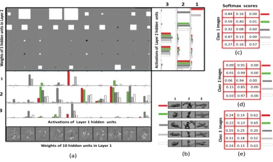
RFs learned from the reduced NORB dataset are plotted as im-ages at the bottom part of (a). The intensity of each pixel is proportional to the magnitude of the weight connected to that pixel in the input image with negative value indicating black, positive values white, and the value 0 corresponding to gray. The biases are not shown. The activations of first layer hidden units for the NORB objects presented in (b) are depicted on the bar chart on top of the RFs. The weights of the second layer AE are plotted as a diagram at the topmost part of (a). Each row of the plot corresponds to the weight of each hidden unit of second AE and each column for weight of every hidden unit of the first layer AE. The magnitude of the weight corresponds to the area of each square; white indicates positive, grey indicates zero, and black negative sign. The activations of second layer hidden units are shown as bar chart in the right-hand side of the second layer weight diagram. Each column shows the ac-tivations of each hidden unit for five color-coded examples of the same object. The outputs of Softmax layer for color-coded test objects with class labels (c) "fourlegged animals" tagged as class 1, (d) "human figures" as class 2, and (e) "airplanes" as class 3 [1]. . . 40

18 Deep network trained on Reuters-21578 data using (a) DpAE,

(b) L1/L2-NCSAE. The area of each square is proportional to

the weight’s magnitude. The range of weights are scaled to

[-1,1] and mapped to the graycolor map. w = −1 is assigned to

(19)

19 Filters learned from NORB data set using SAE with (a) 100 orig-inal filters (b) 14 examples of very similar filters with their cor-responding indices at the bottom (c) 32 filters resulting from

agglo-SAE withτ=16, and (d) 32 original ﬁlters. Black pixels

indicate negative, and white pixels indicate positive weights [2]. 51

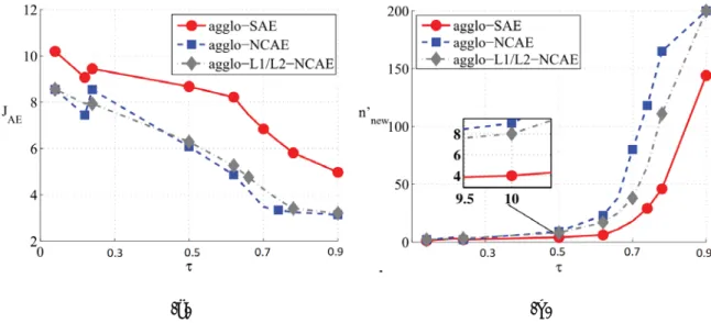
20 Performance of AE on the NORB dataset. (a) Reconstruction

error vs. cluster similarity threshold. (b) Number of RFs vs. cluster similarity threshold for 196 initial ﬁlters [2]. . . 55

21 Reconstruction error using SAE, NCAE, andL1/L2-NCAE trained

with the same number of hidden units from experiment with

agglo-SAE, agglo-NCAE, and agglo-L1/L2-NCAE on NORB data

[2]. . . 55

22 100 receptive ﬁelds learned from Yale Face Dataset using SAE

with examples of two duplicative RFs [2]. . . 56

23 100 receptive ﬁelds learned from Yale Face Dataset using NCAE

with examples of duplicative RFs [2]. . . 56

24 100 receptive ﬁelds learned usingL₁/L2-NCAE from Yale Face

Dataset, with examples of duplicative RFs [2]. . . 57

25 Filters learned from MNIST data set using SAE (a) 200 RFs with

examples of duplicative ﬁlters, (b) 125 RFs for agglo-SAE with

τ=0.6 [2] . . . 57

26 Performance of AE on the MNIST dataset vs. cluster similarity

threshold (a) Reconstruction error (b) RF size (n_new) using 200

(20)

27 Reconstruction error using SAE, NCAE, andL1/L2-NCAE trained

with the same number of hidden units from experiment with

agglo-SAE, agglo-NCAE, and agglo-L1/L2-NCAE on MNIST

data [2]. . . 58

28 KL-Divergence sparsity measure with respect to a desired p

= 0.05 using SAE, NCAE, and L1/L2-NCAE trained with the

same number of hidden units (n_new) from experiment with

agglo-SAE, agglo-NCAE, and agglo-L1/L2-NCAE on MNIST data [2]. 59

29 t-SNE projection [6] of 200D representations of MNIST

hand-written digits using (a) SAE (b) NCAE (c) L1/L2-NCAE, (d)

174D representations using agglo-SAE (e) 153D representations using NCAE, and (f) 172D representations using

agglo-L₁/L₂-NCAE [2]. . . 60

30 Pruning schema of lth layer. (a) Assume ﬁlters red, blue, and

green in the ﬁrst, third, and ﬁfth columns ofW(l), respectively,

are very similar and are located in the same cluster (b) If ﬁlter red is sampled as the representative of the cluster, ﬁlters blue and green are redundant and their corresponding feature maps

in Z₁₊₁ and related weights in the next layer (third and ﬁfth

rows ofW(l+1)) are all pruned [3]. . . 76

31 Average number of redundant features across all layers ( ¯nr)

against thresholdτ with (a) one (b) two (c) three, and (d) four

hidden layers using MNIST dataset. Network width corre-sponds to the number of hidden units per layer and network depth corresponds to number of hidden layers. Networks with more than one hidden layer have equal number of hidden units in all layers. . . 85

(21)

32 t-SNE projection [7] of the activation of last layer of network with (a) one and (b) four hidden layers using 5000 MNIST hand-written digits test samples. All Networks have 1000 hidden units in all layers and all layers use Sigmoid activation function. 86

33 Number of nonredundant ﬁlters (n_f) vs. cluster similarity

thresh-old (τ) for VGG-16 trained on the CIFAR-10 dataset. Initial

number of ﬁlters for each layer is shown in the legend [3]. . . . 88

34 Sensitivity to pruning (a) redundant ﬁlters (b) randomn−n_f

ﬁlters, and (c) redundant ﬁlters and retraining for 30 epochs for VGG-16 [3]. . . 90

35 Number of nonredundant ﬁlters (nf) vs. cluster similarity

thresh-old (τ) for ResNet-56 trained on the CIFAR-10 dataset. Initial

36 Number of nonredundant ﬁlters (n_f) vs. cluster similarity

thresh-old (τ) for ResNet-110 trained on the CIFAR-10 dataset. Initial

37 Sensitivity to pruning n−n_f redundant convolutional ﬁlters

in ResNet-56 [3]. . . 98

38 Sensitivity to pruning n−n_f redundant convolutional ﬁlters

in ResNet-110 [3]. . . 100

39 Illustration of effect of divReg withλ = 10 and τ =0.1 (a) on

three toy ﬁlters in (b) iteration 1 (c) iteration 2 and (d) iteration 4 [4]. . . 107

40 Effect of (a) diversity penalty factorλand (b) thresholding

pa-rameterτon diversity regularization costJ_D(Figure best viewed

(22)

41 The distribution of pairwise feature correlation (Ω(1)) in ﬁrst hidden layer at (a) epoch 2 (b) epoch 300 [4] . . . 118

42 The distribution of pairwise feature correlation (Ω(2)) in

sec-ond hidden layer at (a) epoch 2 (b) epoch 300 [4] . . . 119

43 150 out of 256 encoding features (left) learned from MNIST

digit data set with autoencoders using (a) L1, (b) Dropout (c)

orthoReg, and (d) divReg. The range of weights are scaled and mapped to the graycolor map (right) [4]. . . 120

44 Performance of Multilayer Perceptron (with architecture

784-1024-1024-10) regularized using divReg-1 and trained on the

MNIST dataset vs. thresholdτ∗. (a) Number of nonredundant

features for 1024 initial features. (b) percentage classiﬁcation error [4] . . . 121

45 Evolution of dropout fraction (α) with divReg-2 using the MNIST

dataset for four different initializations of α in (a) layer 1 and

(b) layer 2. Source: [4] . . . 121

46 Performance evaluation using divReg-2 on MNIST dataset for

four different initializations ofα. Source: [4] . . . 127

47 Learning rate (ξ) schedule for experiments on CIFAR-10 dataset.

Source: [4] . . . 127

48 Schema of Diversity Regularized Adversarial Learning (DiReAL)132

49 Diversity loss of (a) generator with no regularization (b)

gener-ator with diReAL (c) discrimingener-ator with no regularization, and (d) discriminator with DiReAL trained on MNIST dataset. . . . 133

50 Divergence, as measured by Wasserstein distance, between the

(23)

51 Synthesized hand-written digits with and without diversity Reg-ularization. . . 134

(24)

INTRODUCTION

Many real-world learning problems involve high-dimensional data and the curse of dimensionality is a fundamental issue. Analysis of data with high dimen-sions usually results in signiﬁcant increase in computational time and space [8, 9]. From practical standpoint, the importance of all features is not the same for a given discriminative task and a good number of features are highly correlated or even re-dundant. This redundancy, in general, would not only increase the computational complexity of the learning process, but also would hinder the interpretability and transparency of the resulting model. However, manual engineering and selection of the most important feature set in high dimensional data for the purpose of elim-inating redundancy is extremely difﬁcult and labor-intensive.

Noticeable research efforts have addressed this issue by designing prepro-cessing and feature extraction pipelines to condition original raw data into forms effectively usable by learning algorithms. However, the process is tedious and requires considerable efforts by experts. In fact, some of the best unsupervised feature extractors (Restricted Boltzmann machines (RBMs) [10], Deep Belief Net-works (DBNs) [11], autoencoders (AE) [12], stacked AE [13], Sparse coding [14], Gaussian Mixture Models (GMMs) [15]) and supervised counterparts (Support Vector Machines (SVM) [16], Gradient Boosting machines (GBMs) [17], neural net-works [18, 19], etc) produce outputs that are unintelligible and inherently hard to decipher their decision making processes. These issues are in fact more prominent when multilayer deep learning (DL) architectures are used. The notion of "deep" in DL does not refer to any kind of deeper understanding/knowledge, rather it refers to the learning of many layers or hierarchies of feature representations. Therefore,

(25)

most of the existing DL models can only be used as black-boxes despite their good performance because their knowledge is hidden and can hardly be used to explain their decision making process. Thus limiting their applicability in domains where both justiﬁcations of decisions and interpretable inference are required from ma-chines as in medical applications and business intelligence [20].

Most of the problems associated with interpretability and computational efﬁciency especially in DL models have been attributed to huge number of param-eters, high nonlinearity, and redundancy in input and/or weight spaces [21], [22] [23], [24]. Therefore, designing a fully trainable algorithms that have the capability to learn the appropriate interpretable features and simultaneously eliminate re-dundancy in both input and model is a step towards solving a long-standing open problem of obtaining an optimal architecture that balances accuracy, memory de-mand, and interpretability.

The following five chapters of this dissertation cover important methods in constrained feature learning and data representation, describe methods of training interpretable features, and discuss algorithms to improve post-training inference cost of DNN models. Chapter II starts by describing some of the theoretical foun-dations of representation learning via constrained data matrix decomposition. It then describes some of the main methods for unsupervised feature extraction in artificial neural networks and the concept of receptive fields (RFs). It also explains how interpretable models can result from the extraction of additive part-based fea-tures. It ends with presenting of two approaches for achieving part-based data de-composition with neural networks and highlights some of their tradeoffs in terms of part-based data decomposition and accuracy.

Chapters III focuses on improving the interpretability of autoencoder-based DNN model while preserving the output accuracy. A novel method for impos-ing non-negativity constraints on RFs is introduced to learn interpretable and

(26)

dis-criminative features. It focuses on methods that preserves the accuracy of mod-els with interpretable features. Chapters IV and V describe methods that seek to eliminate redundancy in both supervised and unsupervised neural network via RF compression. Chapter IV presents two methods for unsupervised learning of non-redundant sparse RFs to improve both computation and accuracy in the su-pervised phase. Chapter V presents two methods for improving the post-training computational efﬁciency of supervised deep convolutional neural networks, also via elimination of redundant RFs. A novel method for imposing diversity among RFs during training is presented and discussed in chapter VI to prevent redun-dancy.

(27)

CHAPTER I

CONSTRAINED FEATURE LEARNING

Constrained feature learning (CFL) is an important concept in feature en-gineering for unearthing latent representations of data useful for such machine learning tasks as classification, regression, and compression. These representa-tions could reveal what is important in data for a given discriminative task. CFL algorithms that enable feature extraction can generate latent codes for test set dur-ing inference [25,26]. CFL algorithms have become important tools in paradigm of representation learning. These algorithms range from sparse coding concept orig-inally introduced in [14] to Nonnegative Matrix Factorization (NMF) that enforces nonnegativity of both basis vectors and the features to neural networks that im-plement learning with a variety of constraints. They are able to learn constrained representation usually by learning some dictionaries that represents the data. The term dictionary is often used in the context of semantic analysis such as document categorization. When dealing with other tasks and data, these dictionaries are called receptive fields, filters, basis vectors or latent factors.

A. Dictionary Learning via Sparse Coding

Dictionary learning is best illustrated through sparse coding or data matrix

factorization. Assume data matrix Xcontains m data vectorsxj as columns, each

with n elements as shown in Fig. 1. Sparse coding aims to ﬁnd a set of k basis

(28)

FIGURE 1 – Illustration of Data Matrix Factorization (X ≈ ΦA). Xis the data

ma-trix, columns of Φ are basis vectors, and columns of A are the encodings of the

samples [5].

A ∈ Rk×m) such thatX ≈ ΦAforX ∈ Rn×m, andajis a sparse vector for every j.

When no limitation is imposed onk, it is possible to ﬁnd via sparse coding an

over-complete representation of data in which the number of basis vectorsk is greater

than the original data dimensionalityn. That is, ifk>nthe linear system of

equa-tions is under-determined and sparsity enforcement is needed to avoid obtaining a trivial solution [26].

In order to coercea_jto be sparse for every j, a sparsity term is introduced in

the objective function. Sparse combination of basis from an over-complete dictio-nary to represent data has been suggested as the mechanism with which mammal primary visual cortex (V1) work [14,27–30]. The data matrix decomposition is usu-ally formulated as an optimization problem solvable by balancing out the error of

approximation of X by ΦA and the sparsity of A. During the optimization

pro-cess, a trivial solution may result in which entries of A are small due to sparsity

enforcement but are compensated by allowing entries of Φ to assume large

val-ues [27,31,32]. To alleviate this problem, magnitude constraints are usually placed

on the basis vectorsφithrough a process known as regularization by adding decay

term to the objective function. This magnitude constraint is sometimes referred to as a weight decay penalty. Most sparse coding methods [14, 27, 33] require solv-ing iterative optimization problem in order to compute feature descriptor which is

(29)

usually computational expensive [26]. The complete optimization objective is thus formulated as in (1). min A,Φ m

∑

j=1 _Φ_a_j₋_x_j2 2+γ1Sparsity(aj) +γ2 k

∑

i=1 φi2 2 (1)

whereγ1andγ2are positive constants that adjust the relative importance of

spar-sity and magnitude (or regularization) constraints, respectively. Formula (1) mini-mizes the distance between the data and its representation given the learned basis.

B. Dictionary Learning via Nonnegative Matrix Factorization (NMF)

Similar to sparse coding, NMF [34] belongs to a class of CFL paradigm that essential to data analysis such as compression, feature selection, visualiza-tion, just to mention a few [35]. NMF ﬁnds application in many diverse problem space such as computational biology [36–41], blind source separation [42], cluster-ing [43, 44], community detection [45], collaborative ﬁltercluster-ing [46], just to mention a few. One of the motivation behind NMF is that the emergence of part-based representation in human cognition can be conceptually tied to the nonnegativity constraints [34]. The objective of NMF techniques in general is to approximate data

matrix Xwith nonnegative entries with low rank matrixWH, that is,X ≈WHor

simplyX=WH+N. One of the key choices in NMF is the quantiﬁcation of

qual-ity of approximation, which generally depends on error N. The most commonly

used measure is the Frobenius norm of N, which assumes the noise in the data is

Gaussian. Another important consideration in CFL is the assumption on the

struc-ture of factors WandH. For instance, if columns ofWare independent, then the

resulting heuristic become independent component analysis (ICA) [47].

The strict constraint on the structure of factors W and H in NMF is that

(30)

thereby resulting in additive data representation. The hidden structure of data can be unfolded by learning features that have capabilities to extract the data parts. Similar to the data decomposition illustrated in Fig. 1, NMF decomposes data

ma-trixX ∈ Rn×m with nonnegative real entries into product of two nonnegative

ma-trices W ∈ Rn×k and H ∈ Rk×m, that is, X ≈ WH. The factorization is generally

formulated as an optimization problem with loss function in (2) min

W∈Rn×k_,_H_∈_Rk×m||X−W H||

2_{such that}_W_≥_{0 and}_H_≥₀

(2)

C. Dictionary Learning via Constrained Autoencoders

Dictionaries are also learnt via a specialized neural network architecture known as autoencoder. One of the popular approaches to CFL is to train autoen-coder (AE) in ways that enforces some desired attributes. The motivation behind the autoencoding is to reconstruct the input from its encoded representation with features that represent the data [48, 49]. The reconstruction is usually achieved by additive linear (sometimes nonlinear) combination through decoding ﬁlters. After training, generating latent encodings for test samples is extremely fast, requiring a simple matrix-vector multiplication.

The model of the neural network AE shown in Fig. 2 aims to reconstruct its input vector using unsupervised learning is given in (3).

ˆ

x= fW,b(x)≈x (3)

where x is a normalized input vector, W = {W1,W2}, and b = {b1,b2}

respec-tively represent the weight and biases of the network. It is worth mentioning that

the weight matrixW2 may optionally be constrained byW2 = WT1, in which case

the autoencoder is said to have tied weights. The concept of tied weights is mainly

(31)

x1 x2 xn−1 xn ˆ x1 ˆ x2 ˆ xn−1 ˆ xn Decoder Encoder h1 hn

Input Layer HiddenLayer

Decoding Layer

b2

b1

W1 W2

FIGURE 2 – Schematic diagram of a three-layer AE

through W1 into features h. In turn, features h are mapped back to the data ˆX

through W2 in accordance with h = σ(W1X+b1) where σ() is the activation

function. One of the commonly used activation functions is the logistic sigmoid

given asσ(x) = 1_/₍1+exp(−x)). In order to solve for parameters Wand bin (3), the

average reconstruction error in (4) serves as the optimization objective.

JAE(W,b) = 1 m m

∑

i=1 σ(W2σ(W1xi+b1) +b2)−xi22 (4)

We should note that the dictionary learning in sparse coding (1) and AE (4) differ by two aspects. Firstly, the reconstruction error (4) involves mapping of data

into itself by two matricesW1 and W2, while the same error being the ﬁrst term

of (1) involves one matrix Φ. Secondly, (1) is solved by optimization, while (4) is

based on unsupervised learning ofh.

Imposing meaningful limitations on network parameters generally forces AE network to learn representations that attempts to unearth the underlying struc-ture in data. One of such limitations could be limiting the hidden layer size for compressed representation of the input. In this context, constrained AE implies that some constraints such as sparsity, nonnegativity, weight-decay

(32)

regulariza-tion, and/or other constraint types are imposed on the learned features. Exam-ples of such constraints are sparsity as in the Sparse Autoencoder (SAE) [50], or nonnegativity and sparsity as in Nonnegativity-Constrained Autoencoder (NCAE) [1, 51, 52].

Sparsiﬁcation of features that represent data is increasingly important in learning, especially from big data. This is because sparsity can facilitate efﬁcient and automatic feature selection. In addition, regularization can shrink the mag-nitude of AE weights and improve the generalization. Therefore, constrained AEs are not only used for feature dimensionality reduction, but also for extract-ing sparse, part-based features, and for enhancextract-ing data understandextract-ing.

1. Constrained Autoencoders for Sparse Representation

In AE settings, a network is considered over-sized if the size of the hidden

layer is the same or larger than the input vector size n. In this scenario, AE can

be forced to learn useful representation if additional constraints are added. These constraints can come in form of regularization to ensure sparsity of the hidden-layer representation or addition of noise in the hidden hidden-layer. Sparse representation can provide a interpretation of the input data in terms of a reduced number of parts thereby revealing its hidden structure.

In order to force AE to learn sparse representation,his bounded using the

Kullback-Leibler (KL) divergence function [53–56]. Ifh_j(xi) denotes the activation

(or output) of hidden neuron j due to the input xi, the average activation of this

particular neuron is given as: ˆ p_j = 1 m m

∑

i=1 h_j(xi) (5)

If a sparse AE with target activation p is considered, one common method for

(33)

[50] as in (6) Sparsity(p||pˆ) = n

∑

j=1 plog p ˆ p_j + (1−p)log 1−p 1−pˆ_j (6)

One of many functions a regularizer provides is enforcing certain properties on the weights. Note that weight decay term is also added to the cost function of AE as to prevent overﬁtting [57]. For a conventional sparse autoencoder (SAE) the decay term is given as in (7). Decay(w) = α 2 2

∑

l=1 sl

∑

i=1 sl+1

∑

j=1 ||w(_i_,l_j)||2₂ (7)

where α is the weight penalty factor, and w(_i_,l_j) represents the connection between

ith neuron in layerl−1 and jth neuron in layerl. The overall cost function based

on (1) for SAE using penalization then becomes [50]:

J_SAE(W,b) = J_AE(W,b) +βSparsity(p||pˆ) +Decay(w) (8)

whereβcontrols the sparsity penalty term.

The gradient of (8) is computed in (11) for the purpose of updating the net-work parameters using the backpropagation algorithm [18].

w(_ijl) =w(_ijl)−ξ ∂ ∂w(_ijl)JSAE(W,b) (9) b_i(l) =b(_il)−ξ ∂ ∂b_i(l)JSAE(W,b) (10) where ∂ ∂w_ij(l)JSAE(W,b) = ∂ ∂w(_ijl)JE W,b+β ∂ ∂w(_ijl)Sparsity p pˆ+g(w(_ijl)) ₍₁₁₎

ξ >0 is the learning rate andg(w(_ijl))is called the decay function and it is given as in (12)

(34)

Other popular methods for sparsifying AE features while preventing

over-ﬁtting are the dropout technique [58] and family ofk-sparse AEs [59,60]. In dropout

technique, units and their connections are randomly dropped from the network during training. In effect, dropout tends to prevent neurons from co-adapting

thereby leading to good generalization. The concept ofk-sparse AE relies on

iden-tifying thekneurons with largest activations and setting the rest to zero to prevent

overﬁtting. The k-sparse AE has been found suitable for many dataset because

the valuekcan be tuned to obtain desirable sparsity level in conformity with each

dataset.

2. Constrained Autoencoders for Part-based Data Representation

Part-based representation is a way of decomposing data into parts, which when additively combined regenerate the data [34]. As shown in [34], one way of representing data is by shattering it into various distinct pieces in a manner that additive merging of these pieces can reconstruct the original data. Mapping this intuition to AEs, the idea is to sparsely disintegrate data into parts in the encoding layer and additively process the parts to recombine the original data in the decod-ing layer.

One way to achieve data decomposition with AEs is by using asymmet-ric piecewise linear weight decay function to constrain network parameters to be nonnegative and the resulting network is called Nonnegative Sparse Autoencoder (NNSAE) [61]. Unlike SAE, NNSAE is trained with an online algorithm and tied weights and linear output activation function. It is capable of extracting nonneg-ative features for part-based representation of data. The main difference between

(35)

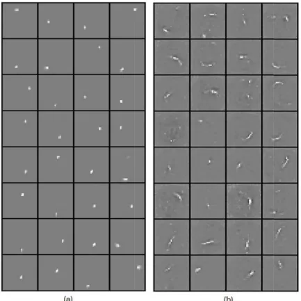
FIGURE 3 – RFs or weights of randomly selected 32 out of 196 (n = 196) hidden neurons of (a) NNSAE (b) NCAE trained using MNIST dataset. Black pixels indi-cate negative, grey pixels indiindi-cate zero-valued weights and white pixels indiindi-cate positive weights. The range of weights are scaled to [-1,1] and mapped to the

gray-color map. w = −1 is assigned to black, w = 0 to grey, andw = 1 is assigned to

(36)

conventional SAE and NNSAE is in the decay function given in (13) g(w(_ijl)) = −αw(_ijl) w_ij <0 −βw(_ijl) w_ij ≥0 (13)

whereαandβare hyperparameters and 0≤α 1. Ifα =1, the decay function in

(13) ensures a complete prohibition of negative weights. The weight decay func-tion in (12) for SAE can also be viewed as imposing Gaussian prior distribufunc-tion on network weights while NNSAE uses a weight decay mechanism that assumes a virtually deformed Gaussian prior that is skewed with respect to the sign of the

weight. It must be noted thatα =β, (13) is equivalent to (12).

Another variant of NNSAE is the Nonnegativity-Constrained AE (NCAE) [51], which also aim at eliminating negative weight through regularization. This is achieved by imposing nonnegativity constraint in form of a penalty term by replacing the decay term in (8) with (14)

Decay(w) = _α 2∑2l=1∑ sl i=1∑ sl+1 j=1 w(_ijl)2 w_ij <0 0 w_ij ≥0 (14)

where α > 0 is a nonnegativity-constraint weight penalty factor and decay

func-tion is given as g(w(_ijl)) = −αw(_ijl) w_ij <0 0 w_ij ≥0 (15) It is worthy to note that the decay function of NNSAE in (13) is a generalization of

both SAE whenβ=αas in (12) and NCAE whenβ=0 as in (15).

Part-based data decomposition is illustrated using NCAE and NNSAE trained on MNIST digit and both AEs have 196 hidden neurons. Weights of trained net-works are portrayed as images of receptive ﬁelds (RFs). Figures 3a and b show the RFs learned by NNSAE and NCAE, respectively. It can be observed that the RFs learned are select parts of handwritten digits such as strokes and dots. The learned featured are localized and tend to look like parts of digits. Part-based

(37)

representation is also illustrated in Figure 4 using NCAE trained on MNIST hand-written characters. NCAE with linear decoder architecture (that is, the activation

functionσ()for decoding layer is identity function) was trained in such a manner

that the column ofW1 are coerced to be sparse. RFs and the decoding ﬁlters are

displayed on the right hand side. A test image of digit 6 shown is ﬁltered through

the network and activationsh are listed. The vector of activations is very sparse

since it only stimulates 4 out of 196 RFs. The test sample can be reconstructed by additively combining four outputs of decoding ﬁlters scaled with magnitudes of

(38)

MNIST HANDWRITTEN DIGITS CHARACTERS

Test sample

[h1, …, h70] = [0.4, 0.0, 0.0,0.0,…, 0.0, 0.6, 0.0,0.0,..., 0.9,0.0, 0.5,0.0,0.0,…, 0.0,0.0]

(Hidden Activations)

|

h

₁

h

34

h

48

h

50

FIGURE 4: Representation of test image as a linear combination of 4 out of 196 constrained RFs and decoding ﬁlters learned from MNIST dataset using NCAE with linear output activation function. Input consist of 784 values corresponding

to a 28×28 pixel image. Only 70 RFs with largest activations to test image "6" and

their corresponding decoding ﬁlters are shown. The RFs and the decoding ﬁlters are rescaled and portrayed as images on the right hand side. Black pixels indicate negative, and white pixels indicate positive weights. The range of weights are

scaled to [-1,1] and mapped to the graycolor map. w = −1 is assigned to black,

(39)

CHAPTER II

CONSTRAINED AUTOENCODERS FOR ENHANCED DATA UNDERSTANDING

It is a general belief that humans analyze complex interactions by breaking them into isolated and understandable hierarchical concepts. Methods for learn-ing understandable models, such as decision tree [62] extract only flat data de-scriptions that lack hierarchical concepts. On the other hand, methods that builds model with hierarchical structure usually extract features that are difficult to un-derstand and/or interpret [63, 64]. As shown in [22], one way to reconcile the requirements of hierarchical organization and easier human understandability of concepts in neural networks is by imposing nonnegative-only weights. Moreover, the emergence of part-based representation in human cognition can be conceptu-ally tied to the nonnegativity constraints [34]. Although deep feedforward neural networks have the capability to model multi-level abstraction of data, they are dif-ficult to train and the understandability of features they learn is very limited [65].

Owing to unsupervised pretraining using AE or Restricted Boltzmann ma-chine [66] and better initialization heuristics [67–70], the training difﬁculties have been alleviated. Some heuristics have also attempted to address the problem of understandability by extracting rules from neural network for individual neurons. These heuristics, however, differentiate rules from individual neuron and their states using special symbols, which in turns increases the opaqueness of the ex-tracted rules. In addition, these symbolic rules becomes more complicated for deep neural networks with no meaningful interpretations. Also, the rule extrac-tion process have been shown to be computaextrac-tionally expensive [21].

(40)

The issue of understandability is addressed by drawing inspiration from the idea of NMF [34] and sparse coding [71] and appropriately enforcing space non-negative features. As highlighted in [22], understandability of features learned by neural network models can be fostered by enforcing weights in the network to be nonnegative. This would allow easier inspection and interpretation by eliminating cancelations of incoming neuron signals. In addition, there are neural activities for a subset of hidden units that are strongly correlated with the input and threshold of this correlation is controlled by the bias term. The main shortcoming in [22] is that sparse nonnegative features are obtained by directly mapping negative weights to zero, in effect, signiﬁcantly deteriorates the performance of the entire network. That is, a portion of the performance is traded with extraction of understandable features. In addition, the heuristic was developed and customized for shallow neural networks. Of special interest to the work in this chapter is the extraction of understandable deep neural network features that preserves the overall network performance.

A. L1/L2-Nonnegativity Constrained Sparse Autoencoder (L1/L2-NCSAE)

As earlier shown using NNSAE [61] and NCAE [51], negative weight can be eliminated from neural network models in an online fashion through regulariza-tion. This is achieved by regularizing the learning cost function with appropriate penalty term. However, a close scrutiny of the weight distribution of both the encoding and decoding layer enforced by the penalty function of NCAE in (14) reveals that many weights are still negative despite imposing nonnegativity

con-straints. The reason for this is that the original L2 norm used in NCAE penalizes

the negative weights with big magnitudes stronger than those with smaller magni-tudes. This forces a good number of the weights to take on small negative values. From experiments carried out using NCAE, these negative weights are essential

(41)

for achieve good performance in terms of both reconstruction and classiﬁcation.

It will be shown that additional L1 term can be used to even out this occurrence,

that is, the additionalL1penalty forces most of the small-valued negative weights

to become zero. The resulting architecture extracts features that are more sparse

with improved reconstruction error and is renamed as L1/L2-Nonnegativity

Con-strained Sparse Autoencoder (L1/L2-NCSAE). The penalty term of NNSAE [61] in

(13) on the other hand also extracts strictly nonnegative feature, however, it does so in a way that deteriorates the classiﬁcation accuracy when used to pretrain a deep network due of its relatively high reconstruction error.

In order to encourage higher degree of nonnegativity in network’s weights, a penalty term in (16) is added to the objective function resulting in the cost

func-tion expression for L₁/L₂-NCSAE [1]. The negative weights are regularized by

minimizing their absolute values (L₁norm) and their squares (L₂norm). The

com-bined action of the L1 and L2 penalties is that they both select only the important negative weights and limits their magnitude. This thus employ a penalty-based negative weight pruning mechanism.

Decay(w_ij) =

α1Γ(wij,κ) + α22||wij||2 wij <0

0 w_ij ≥0

(16)

whereα1andα2areL1and L2nonnegativity-constraint weight penalty factors,

re-spectively. The decay functiond(w_ij)is a composite function denoting the

deriva-tive ofDecay(w_ij)(16) with respect tow_ijas in (17).

g(w_ij) =

_α_1∇

wwij+α2wij wij <0

0 wij ≥0

(42)

1. Implication of imposing nonnegative parameters with composite decay func-tion

The graphical illustration of the relation between the weight distribution and the composite decay function is shown in Fig. 6. Ideally, addition of

Frobe-nius norm of the weight matrix (α||W||2_F) in (12) to the reconstruction error

im-poses a Gaussian prior on the weight distribution as shown in curve G3 in

Fig-ure 6a. However, using the composite function in (17) results in imposition of

positively-skewed deformed Gaussian distribution as in curves G1 and G2. The

degree of nonnegativity can be adjusted using parametersα1andα2. Both

param-eters have to be carefully chosen to enforce nonnegativity while simultaneously

ensuring good supervised learning outcomes. The effect ofL1(α2 =0),L2(α1=0)

andL₁/L₂(α1 =0 andα2 =0) nonnegativity penalty terms on weight updates for

weight distributions G₁, G₂ and G₃ are respectively shown in Figure 6c,d, and b.

It can be observed for all the three distributions thatL₁/L₂regularization enforces

stronger weight decay than individualL₁andL₂regularization. Other observation

from Figure 6 is that the more positively-skewed the weight distribution becomes, the lesser the weight decay function.

The consequences of minimizing the reconstruction under the regulariza-tion in (16) are that: (i) the average reconstrucregulariza-tion error is reduced (ii) the spar-sity of the hidden layer activations is increased because more negative weights are forced to zero thereby leading to sparsity enhancement, and (iii) the number of nonnegative weights is also increased. As earlier mentioned, the resultant effect

of penalizing the weights simultaneously with L1 and L2 norm is that they both

select only the important negative weights and limits their magnitude. However,

the L1 norm in (16) and (17) is non-differentiable at the origin, and this can lead

to numerical instability during simulations. To circumvent this drawback, one of

(43)

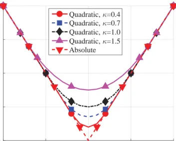
-2 -1 0 1 2 0 0.5 1 1.5 2 Quadratic,κ=0.4 Quadratic,κ=0.7 Quadratic,κ=1.0 Quadratic,κ=1.5 Absolute

FIGURE 5 – Absolute function approximation using quadratic smoothing

func-tions withκ= 0.4, 0.7, 1.0 and 1.5

approximation is deﬁned as follows: Given any ﬁnite dimensional vector z and

positive constantκ, the following smoothing function approximates L1norm:

Γ(z,κ) = ||z|| ||z||>κ ||z||2 2κ +κ2 ||z|| ≤κ (18) with gradient ∇zΓ(z,κ) = z ||z|| ||z||>κ z κ ||z|| ≤κ (19) 2. Experimental Results

a. Unsupervised Feature Learning of Image Data In the ﬁrst set of

experi-ments, three-layer L1/L2-NCSAE, NCAE [51], DpAE [72], and conventional SAE

network with 196 hidden neurons were trained using MNIST dataset of handwrit-ten digits and their ability to discover patterns in high dimensional data are

(44)

com-−1 −0.5 0 0.5 1 0 0.2 0.4 0.6 0.8 1 weight w Probability Distribution P(w) G₁ G₂ G₃ (a) −1 −0.5 0 0.5 1 −2 −1.5 −1 −0.5 0 w g(w) α₁= 1,α₂= 1 α₁= 1,α₂= 0 α₁= 0,α₂= 1 (b) −1 0.5 0 0.5 1 2 1.5 1 0.5 0 w g(w) α₁= 1,α 2= 1 α₁= 1,α₂= 0 α₁= 0,α 2= 1 (c) −0.5 0 0.5 1 1.5 −1.4 −1.2 −1 −0.8 −0.6 −0.4 −0.2 0 w g(w) α₁= 1,α₂= 1 α₁= 1,α₂= 0 α₁= 0,α₂= 1 (d)

FIGURE 6: (a) Symmetric (G₃) and skewed (G₁and G₂) weight distributions.

De-cay function with three values of α1 and α2 for weight distribution (b) G3 (c) G1

(45)

pared. These experiments were run one time and recorded. The encoding weights

W(1), also known as receptive ﬁelds or ﬁlters as in the case of image data, are

re-shaped, scaled, centered in a 28×28 pixel box and visualized. The ﬁlters learned

by L1/L2-NCSAE are compared with that learned by its counterparts, NCAE and

SAE. It can be easily observed from the results in Figure 25 that L1/L2-NCSAE

learned receptive ﬁelds that are more sparse and localized than those of SAE, DpAE, and NCAE. It is remarked that the black pixels in both SAE and DpAE fea-tures are results of the negative weights whose values and numbers are reduced in NCAE with nonnegativity constraints, which are further reduced by imposing an

additional L1 penalty term in L1/L2-NCSAE as shown in the histograms located

on the right side of the ﬁgure. Although the penalty function in NCAE is a special

case of that in L₁/L₂-NCSAE (obtained by setting α1 to zero), a close scrutiny of

the weight distribution of both the encoding and decoding layer in NCAE reveals that many weights are still negative despite imposing nonnegativity constraints.

The reason for this is that the original L₂ norm used in NCAE penalizes the

neg-ative weights with big magnitudes stronger than those with smaller magnitudes.

This forces a good number of the weights to take on small negative values. L₁/L2

-NCSAE uses additionalL₁to even out this occurrence, that is, theL₁penalty forces

most of the negative weights to become nonnegative.

In the case ofL₁/L2-NCSAE, tiny strokes and dots which constitute the

ba-sic part of handwritten digits, are unearthed compared to SAE, DpAE, and NCAE. Most of the features learned by SAE are major parts of the digits or the blurred

version of the digits, which are obviously not as sparse as those learned by L₁/L2

-NCSAE. Also, the features learned by DpAE are fuzzy compared to those ofL1/L2

-NCSAE which are sparse and distinct. Therefore, the achieved sparsity in the

en-coding can be traced to the ability of L1 and L2 regularization in enforcing high

(46)

(a) SAE (b) DpAE (c) NCAE (d) L1 / L2 -NCSAE FIGURE 7: 196 receptive ﬁelds ( W ( 1 ) )learned fr om MNIST digit data set using (a) SAE, (b) DpAE (c) NCAE, and (d) L1 / L2 -NCSAE. Black pixels indicate negative, and white pixels indicate positive weights. The range of weights ar e scaled to [-1,1] and mapped to the graycolor map. w = − 1 is assigned to black, w = 0t og re y, an d w = 1 is assigned to white color [1].

(47)

(a) SAE (b) DpAE

(c) NCAE (d)L1/L2-NCSAE

FIGURE 8: Encoding weights (W(1)) histograms learned from MNIST digit data

set using (a) SAE, (b) DpAE (c) NCAE, and (d)L1/L2-NCSAE [1].

100 200 300 400 500 0 2 4 6 8 10 12

No. of hidden nodes

Reconstruction error SAE NCAE L1/L2−NCSAE DpAE 495 500 1.92 2.1 2.2 2.3 (a) 1000 200 300 400 500 0.02 0.04 0.06 0.08 0.1 0.12 0.14 0.16 0.18

No. of hidden nodes

KL−Divergence SAE NCAE L1/L2−NCSAE DpAE 480 490 500 2 4 6 8x 10 −3 (b)

FIGURE 9: (a) Reconstruction error and (b) Sparsity of hidden units measured by

(48)

(a) SAE (b) DpAE (c) NCAE (d) L1 / L2 -NCSAE FIGURE 10: t-SNE pr ojection [6] of 196D repr esentations of MNIST handwritten digits using (a) SAE (b) DpAE (c) NCAE (d) L1 / L2 -NCSAE [1].

(49)

(a) SAE (b) DpAE (c) NCAE (d) L1 / L2 -NCSAE FIGURE 11: W eights of randomly selected 90 out of 200 receptive ﬁlters of (a) SAE (b) DpAE (c) NCAE, and (d) L1 / L2 -NCSAE using NORB dataset. The range of weights ar e scaled to [-1,1] and mapped to the graycolor map. w < = − 1i s assigned to black, w = 0t og re y, an d w > = 1 is assigned to white color [1].

(50)

-0.15 -0.1 -0.05 0 0.05 0.1 0.15 0 1000 2000 number μ =-0.0027 * * -0.15 -0.1 -0.05 0 0.05 0.1 0.15 0 1000 2000 number μ =-0.0024 * * (a) -0.6 -0.4 -0.2 0 0.2 0.4 0.6 0.8 0 1000 2000 3000 4000 _number Avg(W 1(i,j))= -0.0026 * -0.6 -0.4 -0.2 0 0.2 0.4 0.6 0.8 0 2000 4000 _number Avg(W 2(i,j))=0.0826 * * (b) -0.5 0 0.5 1 0 5000 10000 _number Avg(W 1(i,j))= 0.0017 -0.5 0 0.5 1 0 5000 10000 _number Avg(W 2(i,j))=0.1573 * (c) FIGURE 12: The distribution of 200 encoding ( W ( 1 ) )and decoding ﬁlters ( W ( 2 ) )weights learned fr om NORB dataset using (a) DpAE (b) NCAE (c) L1 / L2 -NCSAE [1].

(51)

Likewise in Figure 9a,L1/L2-NCSAE with other AEs are compared in terms

of reconstruction error, while varying the number of hidden nodes. As expected, it

can be observed thatL1/L2-NCSAE yields a reasonably lower reconstruction error

on the MNIST training set compared to SAE, DpAE, and NCAE. Although, a close

scrutiny of the result also reveals that the reconstruction error of L1/L2-NCSAE

deteriorates compared to NCAE when the hidden size grows beyond 400.

How-ever on the average,L1/L2-NCSAE reconstructs better than other AEs considered.

It can also be observed that DpAE with 50% dropout has high reconstruction error when the hidden layer size is relatively small (100 or less). This is because the few neurons left are unable to capture the dynamics in the data, which subsequently results in underﬁtting the data. However, the reconstruction error improves as the

hidden layer size is increased. Lower reconstruction error in the case of L₁/L₂

-NCSAE and NCAE is an indication that nonnegativity constraint facilitates the learning of parts of digits that are essential for reconstructing the digits. In

ad-dition, the KL-divergence sparsity measure reveals that L₁/L₂-NCSAE has more

sparse hidden activations than SAE, DpAE and NCAE for different hidden layer

size as shown in Figure 9b. Again, averaging over all the training examples,L₁/L2

-NCSAE yields less activated hidden neurons compared to its counterparts.

Also, using t-distributed stochastic neighbor embedding (t-SNE) to project the 196-D representation of MNIST handwritten digits to 2D space, the

distribu-tion of features encoded by 196 encoding ﬁlters of SAE, DpAE, NCAE, andL₁/L2

-NCSAE are respectively visualized in Figures 10a, b, c, and d. A careful look at Figure 10b reveals that digits "4" and "9" are overlapping in DpAE, and this will inevitably increase the chance of misclassifying these two digits. It can also be ob-served in Figure 10c corresponding to NCAE that digit "2" is projected with two

different landmarks. In sum, the manifolds of digits withL1/L2-NCSAE are more

(52)

out the separating boundaries among the digits more easily.

In the second experiment, SAE, NCAE,L1/L2-NCSAE, and DpAE with 200

hidden nodes were trained using the NORB normalized-uniform dataset. The NORB normalized-uniform dataset, which is the second dataset, contains 24, 300 training images and 24, 300 test images of 50 toys from 5 generic categories: four-legged animals, human ﬁgures, airplanes, trucks, and cars. The training and test-ing sets consist of 5 instances of each category. Each image consists of two

chan-nels, each of size 96×96 pixels. The inner 64×64 pixels of one of the channels

cropped out and resized using bicubic interpolation to 32×32 pixels that form a

vector with 1024 entries as the input. Randomly selected weights of 90 out of 200

neurons are plotted in Figure 19. It can be seen that L1/L2-NCSAE learned more

sparse features compared to features learned by all the other AEs considered. The

receptive ﬁelds learned by L₁/L₂-NCSAE captured the real actual edges of the

toys while the edges captured by NCAE are fuzzy, and those learned by DpAE and SAE are holistic. As shown in the weight distribution depicted in Figure 12,

L₁/L₂-NCSAE has both its encoding and decoding weights centered around zero

with most of its weights positive when compared with those of DpAE and NCAE that have weights distributed almost even on both sides of the origin.

b. Unsupervised Semantic Feature Learning from Textual Data In this

ex-periment DpAE, NCAE, andL₁/L2-NCSAE are evaluated and compared based on

their ability to extract semantic features from text data, and how they are able to discover the underlined structure in text data. For this purpose, the Reuters-21578 text categorization dataset with 200 features is utilized to train all the three types of AEs with 20 hidden nodes. A subset of 500 examples belonging to categories "grain", "crude", and "money-fx" was extracted from the test set. The experiments were run three times, averaged and recorded. In Figure 13, the 20-dimensional