Large-Scale Interpretable Multi-View Learning for Very High-Dimensional Problems with Application to Multi-Omic Data

Title

Large-Scale Interpretable Multi-View Learning for Very High-Dimensional Problems with Application to Multi-Omic Data

Permalink

https://escholarship.org/uc/item/3w7613s4

Author

Shams Solari, Omid

Publication Date

Peer reviewed|Thesis/dissertation

eScholarship.org Powered by the California Digital Library

by

Omid Shams Solari

A dissertation submitted in partial satisfaction of the requirements for the degree of

Doctor of Philosophy in Statistics in the Graduate Division of the

University of California, Berkeley

Committee in charge: Professor Peter J. Bickel, Chair

Professor Haiyan Huang Professor Gary Karpen

Dr. James B. Brown

Copyright 2019 by

Large-Scale Interpretable Multi-View Learning for Very High-Dimensional Problems with Application to Multi-Omic Data

by

Omid Shams Solari

Doctor of Philosophy in Statistics University of California, Berkeley Professor Peter J. Bickel, Chair

We discuss the sparse Canonical Correlation Analysis (CCA) problem in the context of high-dimensional multi-view problems, where we aim to discover interpretable association structures among multiple random vectors via their respective views with an emphasis on setting where the number of observations is too few compared to the number of covariates. Throughout this text, we use the term view define as observations of a random vector on an ordered set of subjects, which is the same for observations of all other random vectors involved in the analysis. We denote each view by Xi ∈Rn×pi, i= 1, . . . , m, wherem is the

number of random vectors, or equivalently number of views.

In the first two chapters we consider linear association structures shared among multiple views, where the objective is to learn sparse linear combinations of multiple sets of covariates such that they are maximally correlated.

In the first chapter we introduce a new approach to the sparse CCA, where we learn the sparsity pattern of the canonical directions in the first stage by casting this problem as two successively shrinking concave minimization programs which are solved via a first-order algorithm, and in the second stage we solve a small CCA problem by considering the sparsity patterns estimated in the first stage. We demonstrate via simulations that, in comparison to other available methods, our approach demonstrates superior convergence properties and capability to recover the underlying sparsity patterns and the magnitudes of the non-zero elements of the canonical directions, as well as, significantly lower computational cost. We then apply our method to a multi-omic environmental genetics study on fruit flies, where we hypothesise about the mechanism of adaptation of this model organism to environmental pesticides.

In the second chapter we tackle a shared short-coming of sparse PCA and sparse CCA methods, which is that, in case of estimating multiple components or canonical directions

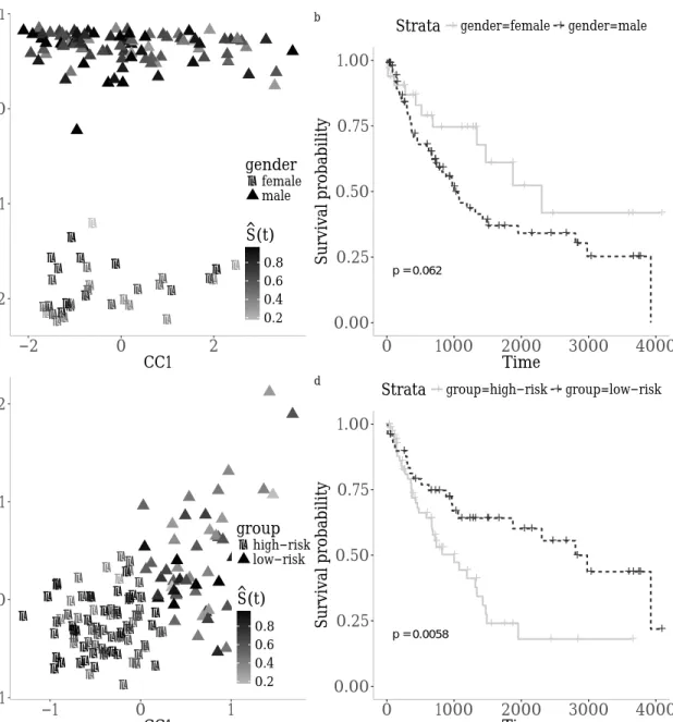
pretability. While all other approaches estimate canonical directions one-by-one via the contraction scheme, we offer a block scheme where we estimate the first d canonical direc-tions simultaneously. In this setting, we can more easily impose orthogonality, and also encourage disjoint sets of non-zero elements within multiple directions, resulting in more interpretable models. We also extended our model to what we call sparse Directed CCA, where we use an accessory variable, defined in the text, to try to capture variations related to a certain hypothesis, rather than the dominant variations which might be proven irrelevant to the main hypothesis. As a validating example, we apply our method to the lung cancer multi-omics available on The Cancer Genome Atlas, using survival data as our accessory variable. While regular sparse CCA exclusively identified correlation structures dominated by and communities separated by gender, our directed sparse CCA correctly identified two underlying communities which were significantly separated by survival.

In the final chapter, we generalize our framework to discover non-linear association structures by proposing a two-stagesparse kernel CCAalgorithm. We learn maximally aligned kernels in the first stage via sparseMultiple Kernel Learning (MKL), and then solve a KCCA problem in the second stage using learned kernels. We perform sparse MKL by forming an alignment matrix where its elements are the sample Hilbert Schmidt Independence Criterion of base kernels of pairs of views. These base kernels are functions of small sets of covariates of each view; therefore our sparse MKL approach provides interpretable solutions, as sparse convex linear combinations of base kernels. We finally provide an Apache Sparkimplementation of our methods introduced throughout the dissertation which makes users capable of running our methods on very high-dimensional datasets, e.g. observations on millions of Single Nucleotide Polymorphism loci, using distributed computing. We call this package SparKLe. R versions of our algorithms are also available. MuLe, BLOCCS, and SparKLe-R implements our methods presented in Chapters 1,2, and 3, respectively.

To my family, That trained me with love!

Contents

Contents ii

1 Sparse Canonical Correlation Analysis via Concave Minimization 1

2 BLOCCS: Block Sparse Canonical Correlation Analysis WithApplication

To Interpretable Omics Integration 45

3 Sparse Multi-View Multiple Kernel Learning with Application to

Chapter 1

Sparse Canonical Correlation Analysis

via Concave Minimization

Abstract

A new approach to the sparse Canonical Correlation Analysis (sCCA) is proposed with the aim of discovering interpretable associations in very high-dimensional multi-view, i.e. observations of multiple sets of variables on the same subjects, problems. Inspired by the sparse PCA approach of Journ´ee et al. (2010), we also show that the sparse CCA formulation, while non-convex, is equivalent to a maximization program of a convex objective over a compact set for which we propose a first-order gradient method. This result helps us reduce the search space drastically to the boundaries of the set. Consequently, we propose a two-step algorithm, where we first infer the sparsity pattern of the canonical directions using our fast algorithm, then we shrink each view, i.e. observations of a set of covariates, to contain observations on the sets of covariates selected in the previous step, and compute their canonical directions via any CCA algorithm. We also introduceDirected Sparse CCA, which is able to find associations which are aligned with a specified experiment design, andMulti-View sCCA which is used to discover associations between multiple sets of covariates. Our simulations establish the superior convergence properties and computational efficiency of our algorithm as well as accuracy in terms of the canonical correlation and its ability to recover the supports of the canonical directions. We study the associations between metabolomics, trasncriptomics and microbiomics in a multi-omic study using MuLe, which is an R package that implements our approach, in order to form hypotheses on mechanisms of adaptations ofDrosophila Melanogaster to high doses of environmental toxicants, specifically Atrazine, which is a commonly used chemical fertilizer.

1. Introduction

Canonical Correlation Analysis(CCA), Hotelling (1935) , is a powerful set of approaches for ana-lyzing the relationship between two sets of random vectors, and discovering associations between elements of said vectors. Classical CCA is specifically concerned with finding linear combinations of the elements of each random vector such that they are maximally correlated estimated using

observations of each random vector on matching subjects/individuals, i.e. different views, of the

same latent random vector. In this article, we use the terms view and dataset interchangeably,

denoted byXi ∈Rn×pi, to refer to nobservations of a random vector of length pi.

CCA has been widely used in various fields of data science and machine learning and has found successful applications in finance, neuro-imaging, computer vision, NLP, social sciences, geogra-phy, collaborative filtering, astronomy and a new surge in genomics, especially in recently popular

multi-assay genetic/clinical population studies. After its proposition by Hotelling (1935), CCA

was first applied inWaugh(1942) where he studied the relationship between the characteristics of

wheat and the resulting flour. He demonstrated that desirable wheat is high in texture, density and protein content and low on damaged kernels and foreign materials. Other rather classic

ap-plications of CCA include: medical geography, where Monmonier and Finn (1973) showed direct

association between the number of hospital beds per capita and physician ratios, socio-medical

studies, e.g. Hopkins (1969) studies the relationship between housing and health in Baltimore,

education, Dunham and Kravetz (1975) analyzes the association between measures of academic

performance in college and exam scores in high school, economics, where Simonson et al. (1983)

employs this technique to identify and describe hedging behavior between the asset side and the

capital side of the balance sheets of a selection of US. banks, signal processing, e.g. Schell and

Gard-ner(1995) introducesProgrammable CCAto design filters to distinguish between desired signal and

noise, time-series analysis, e.g. Heij and Roorda (1991) employs CCA for state-space modeling,

geography, e.g. Ouarda et al. (2001) perform a regional flood frequency analysis using CCA by

investigating the correlation structure between watershed characteristics and flood peaks, medical

imaging, e.g. Friman et al. (2001) benefited from CCA in detecting activated brain regions based

on physiological parameters such as temporal shape and delay of the hemodynamic response. There

are plenty of other examples in the fields of chemistry, e.g. Tu et al. (1989), physics, e.g. Wong

et al. (1980), dentistry, e.g. Lindsey et al. (1985) where CCA is utilized to discover complex yet meaningful associations between two sets of variables.

CCA and its variants have also found substantial grounds in modern fields of research such as artificial intelligence and statistical learning, neuro-imaging and human perception, context-based content retrieval, collaborative filtering, dimensionality reduction and feature selection, and spatial

and temporal genome-wide association studies. Cao et al. (2015) and Nakanishi et al.(2015) used

CCA in the area of Brain Computer Interface(BCI) to recognize the frequency components of target

stimuli. In the area of image recognition,Hardoon et al.(2004) use a kernel CCA method to perform

content-based image retrieval and learn semantics of multimedia content by combining image and

text data. Ogura et al.(2013),Shen et al. (2013), andWang et al.(2013) have employed CCA and

its variants for the purpose of feature selection/extraction/fusion and dimensionality reduction. Modern Canonical Correlation Analysis algorithms have had a significant surge in genomics esp. multi-omic genetic and environmental studies in the last few years mainly due to fast and efficient genome sequencing and measurement technologies becoming more accessible. Such studies typically involve two or more, usually high-dimensional, omic datasets, e.g. trascriptomic, metabolomic,

microbiomic data. An instance of such study is Hyman et al. (2002) where they performed CGH analysis on cDNA microarrays in breast cancer and compared copy number and mRNA expression

levels to infer the impact of genomic changes on gene expression. Yamanishi et al.(2003) successfully

utilized this method to recognize the operons in Escherichia Coli genome by comparing three

datasets corresponding to functional, locational and expression relationships between the genes.

Morley et al. (2004), Pollack et al. (2002), Snijders et al. (2017), Orsini et al. (2018), Fang et al.

(2016),Rousu et al.(2013),Seoane et al.(2014),Baur and Bozdag(2015),Sarkar and Chakraborty

(2015), andCichonska et al.(2016) are few other notable relevant works.

In the next section we provide an overview of the common approaches, but we first compile the notation used throughout the paper in the subsection below.

2. Notation

Each view, i.e. the observation matrix on random vector Xi(ω) : Ω → Rpi, is denoted by Xi ∈

Rn×pi_{, i = 1, . . . , m. n is reserved to denote the sample size and p}

i to denote the length of each

random vector Xi, i = 1, . . . , m. Canonical directions are denoted by zi ∈ Bpi, or zi ∈ Spi, and

Zi ∈ S_dpi, where B = {x ∈ R|kxk2 ≤ 1} and S = {x ∈ R|kxk2 = 1}. lx(z) = kzkx : Rp → R

denotes any norm function, more specificallyl_0/1(z) =_kz_k0/1, andτ(i) _{refers to thei−thnon-zero}

element of the vector which is specifically used for the sparsity pattern vector. Sample covariance

matrices corresponding to thei-th andj-th views is denoted byCij. We drop the subscript when we

only have two views. max(x,0) is also denoted by [x]+. We also coin the term accessory variables

in Section 5.2 to refer to the variables towards which we direct estimated canonical directions,

disregarding their causal roles as covariates or dependent variables. We also use “program” to refer to “optimization programs”.

3. An Overview of Approaches to the CCA Problem

This subsection covers a literature review of Canonical Correlation Analysis, common approaches, and their statistical assumptions and approximations. While linear approaches and especially their regularized extensions are the main focus of this paper, we have also provided an overview of

non-linear approaches, e.g. kernelized model of Lai and Fyfe (2000) and DeepCCA of Andrew et al.

(2013).

3.1 CCA

Let X(ω) : Ω → Rp _{be a random vector with covariance matrix Σ ∈R}p×p_{. Further assume that}

EX=0. Now partitionX intoX1∈Rp1 and X2 ∈Rp2. The covariance matrix can be partitioned

accordingly. Σ= Σ11 Σ12 Σ21 Σ22 (1)

Canonical Correlation Analysis,Hotelling (1935), identifies two weight vectors z1 and z2 such

that the Pearson correlation coefficient between the images X1z1 and X2z2 is maximized,

ρ(z₁∗,z₂∗) = max z1∈Rp_1,z 2∈Rp2 E[(X1z1)>X2z2] E[(X1z1)2]1/2E[(X2z2)2]1/2 = max z1∈Rp_1,z 2∈Rp2 z₁>Σ12z2 q z₁>Σ11z1 q z₂>Σ22z2 = max z1∈Rp_1,z 2∈Rp2 zT 1Σ11z1=1 zT 2Σ22z2=1 z₁TΣ12z2 (2)

where the last line is due to scale-invariability of ρ.

The images X1z1 and X2z2 are called the canonical variables and the weights z1 and z2 are

thecanonical loading vectors or thecanonical directions. The loading vectors (z(1)₁ ,z(1)₂ ) obtained

from optimizing Program2 reveal the first canonical correlation. (z₁(2),z₂(2)) that maximize 2 but

with an added constraint that their corresponding images are respectively orthogonal to the first pair determine the second canonical correlation. This procedure is continued until no more pairs

are found. The number r _≤min_{p1, p2} of pairs of canonical variables can be interpreted as the

number of patterns in the correlation structure.

We estimate the population parameters by plugging in sample estimates of the expectations

in Program 2. With X1 ∈ Rn×p1 and X2 ∈ Rn×p2 being the sample matrices corresponding to

X1 and X2 respectively, Σij, i, j ∈ {1,2} is estimated by the sample covariance matrices Cij =

1

nXi>Xj, i, j∈ {1,2}.

Therefore the sample CCA optimization problem may be written as, max z1∈Rp_1,z2∈Rp₂ z> 1C11z1=1 z> 2C22z2=1 z>₁C12z2 (3)

Generally, this optimization problem is solved using one of the three classes of techniques.

Hotelling(1935) solves this problem using Lagrange multipliers to obtain the characteristic equation

which is a standard eigenvalue problem,

C₂₂−1C21C11−1C12−1z2 =ρ2z2 (4)

Bach and Jordan(2002) andHardoon et al.(2004) form the following system of equations using the same Lagrange multiplier technique,

0 C12 C21 0 z1 z2 =ρ C11 0 0 C22 z1 z2 (5)

Which can be regarded as a generalized eigenvalue problem and the positive generalized

Healy(1957) andEwerbring and Luk(1989) usedsingular value decompositionto find canonical

correlations. In this approach, inverse square roots of the sample covariance matrices C₁₁−1/2 and

C₂₂−1/2 are computed. Canonical loading vectors are computed using the following SVD,

C₁₁−1/2C12C22−1/2 =U DV> (6)

WhereU andV are orthonormal matrices and the non-zero elements of the diagonal matrixD

correspond to the singular values which are equal to the canonical correlations. z₁(k) and z₂(k) are

obtained usingC₁₁−1/2U.k and C22−1/2V.k respectively.

3.2 Regularized CCA

Techniques reviewed above are applicable in over-determined systems or low-dimensional regimes.

However, in high-dimensional regimes where there are fewer observations than variables, n ≤

max_{p1, p2}, new approaches are needed to overcome the issues of singular covariance matrices

and overfitting as well as lack of identifiability of original parameter. These approaches are also helpful in reducing the estimation variance, providing robustness to outliers, and, of special rele-vance to this paper, offering more interpretable models.

3.2.1 Ridge Regularization

So called canonical ridge was proposed in Vinod (1976) to address the problem of insufficient

sample size. Here, the innvertibility of the sample covariance matrices C11 and C22 is improved

by introducing ridge penalties, which comes at the cost of introducing two more hyper-parameters,

c1, c2 ≥0. Ultimately, the optimization constraints in Program 3 become

z>₁(C11+c1I)z1 =1

z>₂(C22+c2I)z2 =1

(7)

Any of the three algorithms of Section 3.1may be modified for solving this problem.

3.2.2 Lasso Regularization

LASSO or L1 regularized CCA, which is one of the two main foci of this paper, is specifically

useful when there are not nearly as many observations as covariates. In such high-dimensional settings ridge-regularized methods, although successfully reducing instability, lack interpretability and overfitting is still an issue. To this end, a school of methods exist which does both variable selection and estimation simultaneously or sequentially through sparsity inducing regularization.

Parkhomenko et al.(2007), Parkhomenko et al.(2009) , andWitten and Tibshirani (2009) advise

a simple soft-thresholding algorithm to enforce sparsity. They apply sparse CCA methods to find

meaningful associations between genomic datasets, be it RNA expression datasets, single-loci DNA

modifications or regions of loss/gain within the genome. Waaijenborg et al. (2008) incorporates a

combination ofL1 and L2 penalties into the CCA model to identify gene networks that are

influ-enced by multiple genetic changes. Hardoon and Shawe-Taylor(2011) offers a different formulation

using convex least squares. In their approach the association between the linear combination of one view and the Gram matrix of the other view is computed. They demonstrate that in cases

when the observations are very high-dimensional, their sparse CCA approach outperforms KCCA significantly.

The approaches to the L1 regularized CCA proposed in the literature referenced above are

almost identical, except for that of Hardoon and Shawe-Taylor (2011). Despite small differences,

e.g. Waaijenborg et al. (2008) uses elastic net which is a mixture of LASSO and ridge penalties, they all solve a regularized SVD using alternating maximization of slightly different optimization

programs. Penalized Matrix Decomposition(PMD) algorithm which was first introduced in Witten

et al.(2009), then extended inWitten and Tibshirani(2009) estimates the sample covariance matrix

C12 with closest rank-one matrix in a Frobenius norm sense under some constraints.

(z₁∗,z₂∗) = arg min z1∈Bp_1,z2∈Bp₂ kz1k1≤c1,kz2k1≤c2,σ≥0 kC12−σz1z2>k2F = arg max z1∈Bp_1,z 2∈Bp2 kz1k1≤c1,kz2k1≤c2 z₁>C12z2 (8)

where ci ≥0, i= 1,2 are sparsity parameters. The last statement in Program 8 is of course a

penalized SVD.

3.2.3 Cardinality Regularization

Most approaches to the sparse CCA problem involve the LASSO regularization which was reviewed

in Section3.2.2. However, few greedy approaches were also developed cardinality orL0 regularized

case. (z₁∗,z₂∗) = arg max z1∈Bp_1,z2∈Bp₂ kz1k0≤c1,kz2k0≤c2 z₁>C12z2 (9)

where as before the sparsity parameters are non-negative. Wiesel et al. (2008) develop a greedy

algorithm which is based on the sparse PCA approach ofd’Aspremont et al.(2008), which we also

base our L0 regularized algorithm on, and demonstrate the effectiveness of their backward greedy

algorithm in high-dimensional settings.

3.3 Bayesian CCA

Bayesian approaches to CCA were introduced to increase the robustness of the model in low sample

size scenarios and improve the validity of the model by allowing different distributions. Klami et al.

(2012) offer a detailed review of Bayesian approaches to CCA, and Bach and Jordan (2005) offer

a formalization of this problem within a probabilistic framework. In these models latent variables

U _{∼ N}(0, Il) where l ≤ min{p1, p2} are assumed to generate the observations x(1i) ∈ Rp1 and

x(₂i)_∈Rp2 _through

X1|U ∼ N(S1U+µ1,Ψ1)

X2|U ∼ N(S2U+µ2,Ψ2)

(10)

where S1 and S2 are transform matrices and Ψ1 and Ψ1 noise covariance matrices. Maximum

3.4 Non-Linear Transformations

So far, our discussion of CCA and its extensions were constrained to linear transformations of observed random variables. Analyzing non-linear correlation structures, however, requires further

innovation. (Deep) neural networks(DNN) based CCA and kernel CCA are reviewed as the two

main schools of methods for uncovering non-linear canonical correlations.

3.4.1 DNN-Based CCA

Lai and Fyfe(1999) used neural networks to find non-linear canonical correlation and detect shift

information in a random dot stereogram data. Lai and Fyfe (2000) extends this by adding a

non-linearity to their network and also by non-linearly transforming the data to a feature space and

then performing linear CCA. Andrew et al. (2013) developed the packagedeepCCA, which will be

explained here briefly. In this approach, each dataset, Xi, is transformed through multiple layers

by applying sigmoid functions on linear transformation of the input to the layer j = 1, . . . , J of

networki= 1, . . . , I,

aj_i =σ(Z_ijxi+bji), i= 1, . . . , I, j= 1, . . . , J (11)

whereσ is a nonlinear sigmoid function andZ_ij andbj_i are the weight matrices and bias vectors

respectively that need to be learned such that some cost function is minimized. The cost function

they defined was the correlation between the output views of all I datasets. Assuming output

matrices H1 ∈ Ro×n and H2 ∈ Ro×n, define C12 = _n−1₁H˜1H˜2>, C11 = _n−1₁H˜1H˜1> +γ1I and

C22 = _n−1₁H˜2H˜2>+γ2I, where ˜Hi = Hi− 1_nHi1 are the centered output matrices. Also define

T =C₁₁−1/2C12C22−1/2. Then the correlation objective to be maximized can be written as the trace

norm ofT.

corr(H1,H2) =tr(T>T)1/2 (12)

Obviously Hi=f(zij, b

j

i), j = 1, . . . , J.

Using DNNs for multi-view learning is a very active line of research. Recently, models based

on Variational Auto-Encoders(VAE) have become popular[Wang et al.(2016)].

3.4.2 Kernel CCA & The Kernel Trick

Kernel methods are more popular for analyzing non-linear associations[Lai and Fyfe(2000)]. This is for the most part due to the vast theoretical literature on kernel methods, mainly from SVM

lit-erature, [Gestel et al.(2001);Cai(2013);Blaschko et al.(2008);Hardoon and Shawe-Taylor(2009);

Alam et al. (2008)] and part due to the significantly fewer number of parameters to be estimated

compared to DNNs[Akaho (2001)]. Melzer et al. (2001) applies non-linear feature extraction to

object recognition and compares it to non-linear PCA. Bach and Jordan (2002) uses CCA based

methods in kernel Hilbert spaces for Independent Component Analysis(ICA) and present efficient

computation of their derivatives. Larson et al. (2014) utilizes kernel CCA to discover complex

multi-loci disease-inducing SNPs related to ovarian cancer.

Kernelized methods use non-linear mappings,φ1(X1) andφ2(X2), of observations to non-Euclidean

spaces,_H1andH1, where the measures of similarity between images are no longer linear. The

product in Hilbert spaces. In essence, KCCA first transforms the observations into Hilbert spaces

H1 and H2 using PSD kernels,

k1(x1i,x1j) =hφ1(x1i), φ1(x1j)iH1, k2(x2i,x2j) =hφ2(x2i), φ2(x2j)iH2 (13)

In practice, we don’t need to specify the mappings φi(xi,j). Mercer’s theorem[Mercer (1909)]

guarantees that as long as k1(xij,x0_ij) is a positive semi-definite inner-product kernel, there is a

corresponding φi : Rpi → H equipped with inner-product < ., . >H. This permits us to bypass

evaluatingφiand go straight to evaluating inner-product kernelski,1, . . . , I. The rest of the analysis

will be quite similar to the CCA problem except that the observation matricesXi are replaced by

their corresponding Gram matrices Ki fori= 1, . . . , I. For a more comprehensive treatment, refer

toHardoon et al.(2004) and Bach and Jordan (2002).

The remainder of this paper is organized as follows: In Section4 we introduce the optimization

problems corresponding to L0/L1regularized CCA which are then extended to Multi-View Sparse

CCA and Directed Sparse CCA in Section 5. In Section 6, we propose algorithms that solve

the optimization programs of Sections 4 and 5. In Section 7 we apply MuLe, the R-package that

implements our algorithms, to simulated data, where we benchmark our method and also compare

it to several other available approaches. We also utilize it in Section 8 to discover and interpret

multi-omic associations which explain the mechanisms of adaptations ofDropsophila Melanogaster

to environmental pesticides. We conclude this paper in Chapter 9. Appendices are referenced in

the text wherever applicable.

4. Sparse Canonical Correlation Analysis

We considersparse CCAformulations of the following form,

φlx,lx(γ1, γ2) = max

z1∈Bp1zmax2∈Bp2z

T

1C12z2−γ1lx(z1)−γ2lx(z2) (14)

where lx = lx(z) is a sparsity-inducing norm function, γi ≥ 0, i = 1,2 are regularization

parameters, andC12= 1/nX1>X2 is the sample covariance matrix.

4.1 L1 Regularization Considerx= 1 in Program 14, φl1,l1(γ1, γ2) = max z1∈Bp_1zmax_2∈Bp₂z T 1C12z2−γ1kz1k1−γ2kz2k1 (15)

This optimization program is equivalent1 to the one in8.

Theorem 1 Maximizers, (z∗₁,z∗₂), of φl1,l1(γ1, γ2) in Program 15 are given by,

z₁∗ = arg max z1∈Bp₁ p2 X i=1 [|cT_i z1| −γ2]2+−γ1kz1k1 (16)

1. Optimization programsψx(λ) andηy(µ) are calledequivalent if there is a one-to-one mappingg:Dλ→ Dµsuch thatx∗_=y∗_ifλ=g(µ).

and z₂∗_i =z∗_2i(γ2) = sgn(c T i z1)[|cTi z1| −γ2]+ qPp2 k=1[|cTkz1| −γ2]2+ , i= 1, . . . , p2. (17) Proof 2 φl1,l1(γ1, γ2) = max z1∈Bp_1zmax_2∈Bp₂z > 1C12z2−γ1kz1k1−γ2kz2k1 = max z1∈Bp1zmax2∈Bp2 p2 X i=1 z2i(c>i z1)−γ2kz2k1−γ1kz1k1 = max z1∈Bp_1zmax₀ 2∈Bp2 p2 X i=1 |z₂0_i|(|c>_i z1| −γ2)−γ1kz1k1 (18)

where we used the following change-of-variable z2i =sgn(c>i z1)z02i. We optimize 18 for z02 for

fixedz1 and change it back toz2 to get the result in Equation17. Substituting this result back in

18, φ2_l1,l1(γ1, γ2) = arg max z1∈Bp₁ p2 X i=1 [_|cT_i z1| −γ2]2+−γ1kz1k1 (19)

The following corollary asserts that we can provide the necessary and sufficient conditions based

on the solutionz₁∗ in order to find the sparsity pattern of z∗₂, i.e. supp(z∗₂), denoted in this paper

asτ2 ∈ {0,1}p2.

Corollary 2 Given the sparsity parameter γ2 and maximizer z1∗ of the program 19, entries z∗2i,

refer to17, for which _|c>_i z₁∗_{| ≤}γ2 are identically zero.

Proof According to Equation 17 of Theorem1,

z₂∗_i = 0_⇔[_|cT_i z₁∗_{| −}γ2]+= 0⇔ |cTi z1∗| ≤γ2 (20)

We can go further and show that we can talk aboutτ2 without solving forz∗1. Consider Equation

17 once again,

|cT_iz1| ≤ kcik2kz1k2=kcik2 (21)

Hence,z2i = 0 fori∈1, . . . , p2 ifkcik2 ≤γ2 without regard toz∗1.

Program 16 can be viewed as a L1 regularized maximization of a quadratic function over a

compact set. Obviously the objective is not convex, since it’s the difference of two convex functions.

2. We use the technique introduced in Journ´ee et al.(2010) for sparse PCA to carry out the proofs of Theorems1

However, as we will elaborate more Chapter6where we propose our two-stage algorithm,MuLe, we

are only interested inz₁∗ for the purpose of inferringτ2. Hence we will optimize Program19 with

no regularization term in the first stage.

φ2_l1,l1(γ1, γ2)≈ max z1∈Bp1 p2 X i=1 [|cT_i z1| −γ2]2+= max z1∈Sp₁ p2 X i=1 [|cT_i z1| −γ2]2+ (22)

Remark 3 As a result of this approximation, as stated in Program22, the search space is drastically shrunk from a p1-dimensional Euclidean ball to a p1-dimensional sphere. This is as a result of

maximizing a convex function over a compact set.

Remark 4 Program 22is a valid approximation of the Program 19. Beside our simulation results in Section7, we can see that there is a one-to-one mapping γ1 =h(γ2) in light of Equation 20; in

other words, for every γ1 for which z₁∗_i = 0 there is aγ2 for which the last inequality in20 is true.

4.2 L0 Regularization

Adapting formulation9 ofWiesel et al.(2008) to our approach is equivalent to settingx= 0 in14,

φl0,l0(γ1, γ2) = max

z1∈Bp1zmax2∈Bp2z

T

1C12z2−γ1kz1k0−γ2kz2k0 (23)

However, to make use of the results in the previous section, we consider the following program instead,

φ0_l0,l0(γ1, γ2) = max

z1∈Bp_1zmax 2∈Bp2

(z₁TC12z2)2−γ1kz1k0−γ2kz2k0 (24)

Theorem 5 Maximizers, (z∗₁,z∗₂), toφl0,l0(γ1, γ2) in Program 23are given by,

z₁∗= arg max z1∈Bp₁ p2 X i=1 [(cT_iz1)2−γ2]+−γ1kz1k0 (25) and z₂∗_i=z₂∗_i(γ2) = [sgn((cT_i z1)2−γ2)]+c>i z1 qPp2 k=1[sgn((cTkz1)2−γ2)]+(c>kz1)2 , i= 1, . . . , p2. (26)

Proof Consider optimizing over z2 while keeping z1 fixed. First, assume γ2 = 0. Obviously,

φl0,l0(γ1,0)|z1=const. is maximized at z∗2 = c>i z1. Now, considering the case for γ2 > 0, for which

z₂∗_i = 0 for any z1 such that φl0,l0(γ1,0)|z1=const. = (ciTz1)2 ≤ γ2. Considering this analysis and

normalizing we obtain Equation 26. Substituting back in 24, we arrive at 25.

Similar to the L1 regularized case, the following corollary formalizes the relationship between

Corollary 6 Given the sparsity parameter γ2 and solution z1∗ to the program 25,

τ2i=

(

0 ₋√γ2≤c>i z∗1 ≤√γ2

1 otherwise (27)

Proof According to Equation 26 of Theorem5,

z∗_2i = 0_⇔sgn((cT_i z∗₁)2₋γ2)≤0⇔(cTi z1∗)2 ≤γ2 (28)

Again, even without solving for z∗₁ we can show that

(cT_i z1)2 ≤ kcik22kz1k22 =kcik22 (29)

Hence, in light of 26,z2i= 0 fori∈1, . . . , p2 ifkcik22 ≤γ2 without regards to z1∗.

As before, Program25 can be viewed as aL0 regularized maximization of a quadratic function

over a compact set. Also, we are only interested in z₁∗ for the purpose of inferring τ2. Therefore,

to be able to use the previous result in shrinking the search domain, we will optimize Program 25

with no regularization in the first stage.

φ0_l0,l0(γ1, γ2)≈ max z1∈Bp₁ p2 X i=1 [(c>_i z1)2−γ2]+= max z1∈Sp₁ p2 X i=1 [(c>_i z1)2−γ2]+ (30)

The same justifications as presented in Remarks 3and 4 apply here analogously.

So far we proposed methods to infer the sparsity patternsτ1 andτ2 which can be used to shrink the

covariance matrix drastically, as explain in Section6. Now, efficient CCA algorithms may be used

to estimate the active entries ofz₁∗andz₂∗. Assuming we have estimated thei₋thpair of canonical

loading vectors, (z1,z2)(i), i= 1, . . . , I, whereI =rank(C12)≤nassuming n << min{p1, p2}, we

define thei-th Residual Covariance Matrix as,

C₁₂(i)=C12−

i

X

k=1

(z₁(k)∗>C₁₂(k−1)z₂(k)∗)z₁(k)∗z₂(k)∗> 1_≤i_≤I (31)

The (i+ 1)₋thpair of canonical loading vectors are estimated by the leading canonical loading

vectors ofC₁₂(i), using any of the previous two methods. Refer to Algorithm9 in AppendixB.1 for

more details.

5. Further Applications and Extensions

In this section we further extend the methods developed in Section 4. In 5.1 we introduce our

approach toMulti-View Sparse CCA, where more than two views are available. In 5.2 we extend

our approach toDirected Sparse CCA, where an observed variable, other than the observed views,

5.1 Multi-View Sparse CCA

So far we limited ourselves to a pair of views in discussing the sub-space learning problem. In this section we extend our approach to learning sub-spaces from multiple views, i.e. when we have

multiple groups of observations,Xi ∈Rn×pi, i= 1, . . . , mon matching samples. An example of this

problem is multi-omic genetic studies where transcriptomic, metabolomic, and microbiomic data are collected from a single group of individuals. Thus, we try to discover the association structures

between random vectors Xi by estimating zi such that Xizi are maximally correlated in pairs.

Here, we propose a solution to the following optimization program which is equivalent to the one

proposed in Witten and Tibshirani(2009),

φM_lx(Γ) = max zi∈Bpi ∀i=1,...,m m X r<s=2 z_rTCrszs− m X s=2 s−1 X r=1 r6=s Γsrkzsk1 (32)

where m is the total number of available views, Γ ∈Rm×m_{, Γ}

ij ≥0 is a Lagrange multiplier

matrix, andCrs= 1/nXrTXsis the sample covariance matrix of the (r, s) pairs of views. Following

similar procedure as in4.1, we analyze the solution to Program32.

Theorem 7 The local optima z∗₁, . . . ,z_m∗ of the optimization problem 32 is given by,

z_si∗ =z_si∗(Γ) = sgn(Pmr=1 r6=sc˜ > rsizr)[|Pmr=1 r6=sc˜ > rsizr| −Pmr=1 r6=sΓsr]+ rPp2 k=1[| Pm r=1 r6=sc˜ > rskzr| − Pm r=1 r6=sΓsr] 2 + (33)

and for r = 1, . . . , m andr ₆=s,

zr(Γ) = max zr∈Bpr r6=s,r=1,...,m ps X i=1 [| m X r=1 r6=s ˜ c>_rsizr| − m X r=1 r6=s Γsr]2++ m X i<j=2 i,j6=s z_i>Cijzj− m X i=1 i6=s m_X−1 j=1 i6=j Γijkzik1 (34)

φm_l1(Γ) = max zr∈Bpr r6=s,r=1,...,m max zs∈Bps m X r<s=2 z>_rCrszs− m X s=1 m_X−1 r=1 r6=s Γsrkzsk1 (35) = max zr∈Bpr r6=s,r=1,...,m max zs∈Bps ps X i=1 zsi( m X r=1 r6=s ˜ c>_rsizr)− m X r=1 r6=s Γsrkzsk1+ I z }| { m X i<j=2 i,j6=s z_i>Cijzj− m X i=1 i6=s i−1 X j=1 i6=j Γijkzik1 (36) = max zr∈Bpr r6=s,r=1,...,m max zs∈Bps ps X i=1 |z_si0 _|(_| m X r=1 r6=s ˜ c>_rsizr| − m X r=1 r6=s Γsr) +I (37)

The last line follows fromzsi =sgn(Pmr=1

r6=sc˜

>

rsizr)zsi0 . ˜crsi=crsi ifr < s, and ˜crsi =c>rsi ifr > s

wherecrsi is the ith row ofCrs= 1/nXrTXs. Solving forzs0 and converting back to zs, using the

aforementioned change-of-variable and normalizing, we get the local optimum in 33. Substituting

back to37, φm_l12(Γ) = max zr∈Bpr r6=s,r=1,...,m ps X i=1 [| m X r=1 r6=s ˜ c>_rskzr| − m X r=1 r6=s Γsr]2++ m X i<j=2 i,j6=s z>_i Cijzj − m X i=1 i6=s m_X−1 j=1 i6=j Γijkzik1 (38)

As pointed out in Section 4.1, we’re only interested in the optimizing 38 in order to find the

sparsity patternτs∈ {0,1}ps. Per Remark4, we can make a good approximation by not considering

the regularization terms, simplifying the problem to,

φm_l12(Γ) = max zr∈Bpr r6=s,r=1,...,m ps X i=1 [| m X r=1 r6=s ˜ c>_rsizr| − m X r=1 r6=s Γsr]2++ m X i<j=2 i,j6=s z>_i Cijzj ₍₃₉₎

Corollary 8 For a sparsity parameter matrix Γ and the solution, z∗_r for r = 1, . . . , m and r ₆=s, to the Program 39, τ2i =    0 |Pmr=1 r6=sc˜ > rsizr| ≤Pmr=1 r6=sΓsr 1 otherwise (40)

Proof Scanning Equation 33,

z_si∗ = 0_⇔[_| m X r=1 r6=s ˜ c>_rsizr| − m X r=1 r6=s Γsr]2+= 0⇔ | m X r=1 r6=s ˜ c>_rsizr| ≤ m X r=1 r6=s Γsr (41) Regardless ofz_r∗ we have, | m X r=1 r6=s ˜ c>_rsizr| ≤ m X r=1 r6=s kc˜rsik2kzrk2 = m X r=1 r6=s kc˜rsik2 (42) Hence,τsi= 0 fori∈1, . . . , ps ifPmr=1 r6=sk ˜ crsik2≤Pmr=1 r6=s Γsr regardless ofzr∗.

Computing τi is the first stage of our two-stage multi-modal sCCA approach, for which a fast

algorithm is proposed in 6.4 as part of our proposed MuLe framework. The second stage of our

approach consists of estimating the active elements of z∗_i, for which we use two methods, one is to

frame the multi-modal CCA problem as a generalized eigenvalue problem as originally proposed in

Kettenring(1971), see AppendixB.2, and the other one is a more algorithmic approach of extending

SVD via power iterations to multiple views, refer to AppendixB.3.

5.2 Directed Sparse CCA

Consider a setting where in addition to the views Xi ∈ Rn×pi, some accessory variable3, Y(ω) :

ω → R y ∈ Rn_{, is also observed. We also term the observed accessory variable the Accessory}

Direction,y_∈Rn. Having observedy, the objective is to find linear combinations of the covariates in each view which are highly correlated with each other and also “associated” with the accessory direction. This is useful in high-dimensional settings where rank-deficient covariance matrices lead to over-fitting, and small sample sizes are not representative of the direction of variance within each population, and particularly useful in hypotheses generation where we’re interested in correlation structures associated with a specific experiment design, e.g. association mechanisms corresponding to a certain treatment effect. Here we compare two approaches to this problem,

5.2.1 Two-Step Formulation

Witten and Tibshirani (2009) propose Sparse Supervised CCA, where they consider an extra ob-served outcome. Their approach consists of two sequential steps where the first step, which is

completely separate from the second step, involves finding subsets Qi of each random vector Xi

3. We coined the termAccessory Variable to prevent confusion about the causal role ofy, and to emphasize that independent from their role, whether dependent or independent variable, we are solely utilizing them as a direction towards which we’re directing the canonical directions.

using a conventional variable selection method, e.g. LASSO regression. In the second step, they utilize sparse CCA where the scope of search and estimation of the canonical directions is limited

to the subspaces defined byXij, j ∈Qi,

φl1,l1(γ1, γ2) = max z1∈Bp1 z1j=0,∀j∈Q1 max z2∈Bp₂ z2j=0,∀j∈Q2 z₁TC12z2−γ1kz1k1−γ2kz2k1 (43)

In AppendixB.4 a simple algorithm to optimize43is introduced. This approach, however, has

two considerable shortcomings:

1. Although the scopes of canonical directions are limited to the subspace spanned by zi ∈

Bpi_{, z}

ij = 0,∀j ∈ Qi, the active elements of these directions are estimated to maximize the

sCCA criterion. The estimated direction may well not be associated to the outcome vector anymore, which misses the point.

2. Computing Qi requires some parameter tuning, e.g. sparsity parameters, which is blind to

the CCA criterion; as a result, Qi might exclude covariates which are moderately correlated

withy but highly associated with covariates in other views.

To bridge the gap between the two stages, we propose an approach whereziare estimated in one

stage such that the canonical covariates are highly correlated with each other and also associated with the accessory variable.

5.2.2 Single-Stage Formulation

The following optimization problem tends to perform the two stages of variable selection and performing sCCA in one stage simultaneously,

φD_l1,l1(γ,) = max z1∈Bp_1zmax_2∈Bp₂z T 1C12z2− 2 X i=1 [iLi(Xizi,y) +γikzik1] (44)

where _Li is some loss function which directs our canonical directions to be associated with

the accessory direction y, and γi, i ∈R, i = 1,2 are non-negative Lagrange multipliers. Here we

analyze two scenarios,

a. Let’s consider the case wherey is another separate explanatory variable. Here, one possible

utility function is the dot-product between the canonical covariates and the explanatory variable,

i.e. L(Xizi,y) =−hXizi,yi. Replacing in 44, we have,

φD_l1,l1(γ,) = max z1∈Bp1 max z2∈Bp2 z₁TC12z2+ 2 X i=1 [iy>Xizi−γikzik1] (45)

Theorem 9 The local optima, (z₁∗,z₂∗), to φD_l1,l1(γ,) in optimization program 45 is given by,

z₁∗ = arg max z1∈Bp₁ p2 X i=1 [_|cT_i z1+2x>2iy| −γ2]2++1yX1z1−γ1kz1k1 (46)

and z₂∗_i =z₂∗_i(γ2, 2) = sgn(cT i z1+2x>2iy)[|ciTz1+2x>2iy| −γ2]+ qPp2 k=1[|cTi z1+2x>2iy| −γ2]2+ , i= 1, . . . , p2. (47) Proof φD_l1,l1(γ,) = max z1∈Bp1 max z2∈Bp2z T 1C12z2+ 2 X i=1 [iy>Xizi−γikzik1] = max z1∈Bp1 max z2∈Bp₂ p2 X i=1 z2i(cTi z1+2x>2iy)−γ2kz2k1+1yX1z1−γ1kz1k1 = max z1∈Bp1 max z2∈Bp2 p2 X i=1 |z0_2i|(_|cT_i z1+2x>2iy| −γ2) +1yX1z1−γ1kz1k1 (48)

As before we used a simple change of variable,z2i=sgn(cTi z1+2x>i y)z20i. We solve 48forz20

for fixedz1 and convert it back, using the aformentioned change-of-variable, toz2 to get the result

in Equation 47. Substituting this result back in48,

φD_l1,l12(γ,) = max z1∈Bp₁ p2 X i=1 [_|cT_i z1+2x>2iy| −γ2]2++1yX1z1−γ1kz1k1 (49)

Quite similar to our sCCA formulation we can find the sparsity pattern,τ2 of z2∗ by looking at

z₁∗.

Corollary 10 Given hyperparametersγ2, 2, and z∗1 from program46,τ2i = 0 if|cT_i z∗1+2x>_2iy| ≤

γ2.

Proof According to Equation 47 of Theorem9,

z∗_2i = 0⇔[|cT_i z₁∗+2x>2iy| −γ2]+= 0⇔ |cTi z1∗+2x>2iy| ≤γ2 (50)

We can go further and show that we can talk aboutτ2 without solving forz1∗,

|cT_i z1+2x>2iy| ≤ kcik2kz1k2+2kx2ik2kyk2=kcik2+2kx2ik2 (51)

Hence,z2i = 0 fori∈1, . . . , p2 ifkcik2+2kx2ik2 ≤γ2 regardless ofz1∗.

b. Let’s examine a setting whereyis an outcome variable. Here the objective is to ideally find a

common low-dimensional subspace in which the projections ofXi are as correlated as possible and

also descriptive/predictive of the outcome y. Being confined to linear projections, we can choose

Li(Xizi,y) =ky−Xizik22, i.e. sum of squared errors loss. Rewriting44with this choice,

φD_l1,l1(γ,) = max z1∈Bp1zmax2∈Bp2z T 1C12z2− 2 X i=1 [iky−Xizik22+γikzik1] (52)

Theorem 11 The optimization program in 52 is equivalent to the following program, φD_l1,l1(γ,) = max z∈Bpz >_Cz˜ _{+ 2y}>_Xz˜ _{−γ1kz1k1−γ1kz2k1 (53)} where, ˜ z= z1 z2 , C˜ = 1C11 C12 C₁₂> 2C22 , X˜ =1X1 2X2, (54)

and p=p1+p2. The solution, (z1∗,z2∗), toφDl1,l1(γ,) in Program 52is given by,

v∗ = arg max v∈Bp p2 X i=1 [_|c˜T_i v+ 2 ˜x>_i y_{| −}γ1I(i≤p1)−γ2I(p1<i)] 2 + (55) and z_i∗ =z∗_i(γ,) = sgn(˜c > i v+ 2 ˜x>i y)[|c˜Tiv+ 2 ˜x>i y| −γ1I(i≤p1)−γ2I(p1<i)]+ qPp k=1[|c˜Tkv+ 2 ˜x>ky| −γ1I(k≤p1)−γ2I(p1<k)]2+ , i= 1, . . . , p2. (56) Proof Let R= ˜C1/2. φD_l1,l1(γ,) = max z∈Bpmax_v∈Bpv >_C˜1/2_{z+ 2y}>_Xz˜ _{−γ1kz1k1−γ2kz2k1} = max v∈Bpmax_z∈Bp p X i=1 zi(˜c>i v+ 2 ˜x>i y)−γ2kz2k1−γ1kz1k1 = max v∈Bpmax_z∈Bp p X i=1 |z_i0|(|c˜>_i v+ 2 ˜x>_i y| −γ1I(i≤p1)−γ2I(p1<i)) (57)

where zi =sgn(˜c>i v+ 2 ˜x>i y)zi0. We optimize57 for z0 for fixed v and express it in terms ofz

to get the result in Equation 56. Substituting this result back in 57,

φD_l1,l12(γ,) = max v∈Bp p X i=1 [_|c˜>_i v+ 2 ˜x>_i y_{| −}γ1I(i≤p1)−γ2I(p1<i)] 2 + = max v∈Sp p X i=1 [|c˜>_i v+ 2 ˜x>_i y| −γ1I(i≤p1)−γ2I(p1<i)] 2 + (58)

The last line follows from the fact that the objective function is convex, and the maximization is over a convex set, therefore the maxima are located on the boundary.

Parallel to the Corollary 10, we can find the relationship between the sparsity pattern τ _∈Rp,

Corollary 12 Solving 58for v∗ given γ and ,

|c˜>_i v∗+ 2 ˜x>_i y_{| ≤}γ1I(i≤p1)+γ2I(p1<i)⇒τi = 0

Proof According to Equation 56 of Theorem11,

|cT_i z₁∗+2x>2iy| ≤γ1I(i≤p1)+γ2I(p1<i)

⇒[|c˜T_i v∗+ 2 ˜x>_i y| −γ1I(i≤p1)−γ2I(p1<i)]+ = 0

⇒τ_i∗ = 0

(59)

We can go further and show that we can talk aboutτ without solving forv∗,

|c˜T_i v∗+ 2 ˜x>_i y_{| ≤ k}c˜ik2+ 2kx˜ik2 (60)

Hence,

τi = 0 if kc˜ik2+ 2kx˜ik2 ≤γ1I(i≤p1)+γ2I(p1<i), f or i= 1, . . . , p. (61)

So far in Sections 5.1 and5.2, new approaches to Multi-View sCCA and Directed sCCA were

introduced. The former was proposed to compute the canonical directions when we have more than two sets of variables, while the latter was proposed to direct the canonical directions towards an accessory direction.

Proposition 13 The Directed sCCA approach in 5.2.2.a is equivalent to the approach in 5.2.2.b assuming an orthogonal design matrix, i.e. cov(Xi) =Ipi, and both are equivalent to the Multi-View

sCCA approach where the inputs are three views X1,X2 and y.

Proof Assuming an orthogonal design, min z∈Bpky−Xzk 2 2 = min z∈Bpy >_y−2y>_Xz+z>_X>_{Xz= max} z∈Bpy >_{Xz= max} z∈Bphy,Xzi (62)

Hence programs 45 and 52 are equivalent. Now considering the multi-view approach for this

problem, φM_lx(Γ) = max zi∈Bpi ∀i=1,...,3 3 X r<s=2 z_rTCrszs− 3 X s=1 2 X r=1 r6=s Γsrkzsk1 = max zi∈Bpi ∀i=1,2,3 z₁TX₁>X2z2+z1TX1>yz3+zT2X2>yz3− 3 X s=1 2 X r=1 r6=s Γsrkzsk1 = max zi∈Bpi ∀i=1,2 z₁TX₁>X2z2+z1TX1>y+z2TX2>y−Γ12kz1k1−Γ21kz2k1 (63)

where the last line follows from the fact that p3 = 1, soz3∗ = 1. Equation63 is identical to 45 for

1 =2 = 1.

6. MuLe

In this section we propose algorithms to solve the optimization programs introduced in Sections4

and 5. We also address the problem of initialization and hyper-parameter tuning. Our proposed

algorithms are generally two-stage algorithms; in the first stage we find the sparsity patterns,

τi ∈ {0,1}pi, i= 1, . . . , m, of the optimal canonical directions via concave minimization programs

introduced before, and in the second stage we shrink the covariance matrices using the sparsity patterns, [C_ij0 ]rs = [Cij]_τ(r)

i τ (s) j

, where τ_i(r) is the r −th non-zero element of τi or r −th active

element ofz_i∗, and solve the CCA problem using anyGeneralized Rayleigh Quotient maximizer.

Remark 14 In order to compute τi for i= 1, . . . , m, we start by computing τm, using which we

shrink Cim ∀i 6= m to [Cim0 ]rs = [Cim]_rτ(s)

m . This in turn shrinks the search space on zm when

computing τi, i 6=m. We perform the same shrinkage sequentially as we move down towards τ1,

shrinking the search space significantly each time. This sequential shrinkage, not only decreases computational cost drastically, it is also very useful in specifically very high-dimensional settings, since as with each shrinkage, we are directing successive solutions away from the normal cones of the preceding one. This might explain superior stability of our algorithm demonstrated in Section

7.

Collecting from previous sections, the main differentiating characteristic of our approach is that we cast the problem of finding the sparsity patterns of the canonical directions as a maximization

of a convex objective over a convex set, which is equivalent to the followingConcave Minimization

problem,

φ∗ = max

z∈Rpf(z) = min_z∈Rp−f(z) (64)

where f :Rp→R is a convex function. ConsultMangasarian(1996) andBenson(1995) for an

in-depth treatment of this class of programs. Journ´ee et al.(2010) propose a simple gradient ascent

algorithm for this problem, for which they provide step-size convergence results. Considering these results as well as its empirical performance in terms of convergence and small memory foot-ptint, we also decided to use the following first-order method,

Algorithm 1:A first-order optimization method.

Data: z0 ∈ Q

Result: z∗= arg max_z∈Qf(z)

1 k←0

2 while convergence criterion is not met do

3 z_k+1 ←arg max_x∈Q(f(z_k) + (x−z_k)Tf0(z_k))

What follows in this section, is the application of Algorithm 1to the programs proposed so far in this paper.

6.1 l1-Regularized Algorithm

Applying algorithm1 to the problem in Program 22.

Algorithm 2: MuLe algorithm for optimizing Program22 Data: Sample Covariance MatrixC12

l1-penalty parameter γ2

Initial valuez1 ∈ Sp1

Result: τ2, optimal sparsity pattern for z∗2

1 initialization;

2 while convergence criterion is not met do 3 z1 ←Ppi=12 [|c>i z1| −γ2]+sgn(c>i z1)ci

4 z1 ← _kzz₁1_k2

5 Outputτ₂ ∈ {0,1}p2 _whereτ

2i= 0 if |c>i z1∗| ≤γ2 and 1 otherwise.

Once the sparsity pattern τ2 is found, we shrink the covariance matrix to C120 ∈ Rp1×|τ2|, as

prescribed at the beginning of this section, and apply Algorithm1toC₁₂0 >to findτ1. Now we shrink

the sample covariance matrix once more toC₁₂00 ∈R|τ1|×|τ2|_{. For large enough sparsity parameters,}

this matrix is no more rank-deficient, and we can use conventional SVD or CCA methods to fill in

the active elements of zi, i.e. solve for the leading singular vectors or canonical covariates of this

much smaller matrix.

6.2 l0-Regularized Algorithm

Now, we use Algorithm 1to optimize Program30.

Algorithm 3: MuLe algorithm for optimizing Program30 Data: Sample Covariance MatrixC12

l1-penalty parameter γ2

Initial valuez1 ∈ Sp1

Result: τ2, optimal sparsity pattern for z∗2

1 initialization;

2 while convergence criterion is not met do 3 z1 ←Pp_i=12 [(c>i z1)2−γ2]+c>i z1ci

4 z1 ← _kzz₁1_k2

5 Outputτ₂ ∈ {0,1}p2 _whereτ

2i= 0 if (c>i z1∗)2 ≤γ2 and 1 otherwise.

Similar to 6.1, we perform successive shrinkage and find τ1 in the nest step by applying

6.3 Algorithm Complexity

Perhaps the most appealing characteristic of our proposed algorithm is its significantly lower time complexity compared to other state of the art algorithms. Here we analyze the time complexity of

MuLe and compare it to the most common algorithm for sCCAwhich is the alternating first order

optimization, e.g. Waaijenborg et al. (2008), Parkhomenko et al. (2009), Witten and Tibshirani

(2009), for which we use the umbrella term sSVD here. Following the set-up thus far, assume

we have observed X1 ∈ Rn×p1 and X2 ∈ Rn×p2 and we wish to recover sparse canonical loading

vectors z1 ∈ Rp1 and z2 ∈ Rp2. In order to create more intuition about the speed-up consider

a hypothetical algorithm which uses power method to solve a SVD problem and finally simply

uses hard-thresholding to create sparse loading vectors. We will call this algorithm pSVDht. Also

consider another hypothetical algorithm calledsSVDhtwhich performs the alternating maximization

and similarly induces sparsity by hard-thresholding.

Proposition 15 Time complexity of each iteration of MuLe is smaller than that of pSVDht if

n < min_{p1, p2} andp1∼p2.

Proof. The proof of Proposition 15 is presented in AppendixA.1.

Proposition 16 The time complexity of each(z1, z2)update of the MuLealgorithm, i.e. Algorithm

2, is significantly lower than that of the sSVD algorithm, Witten and Tibshirani (2009) Algorithm 3.

Proof. A simple proof is provided in Appendix A.2.

6.4 Sparse Multi-View CCA Algorithm

Our sparse multi-view formulation offered in Program 39scales linearly with the number of views,

which along with the immense shrinkage of the search domain as a result of our concave minimiza-tion program results in considerable reducminimiza-tion in convergence time. Below is our proposed gradient

ascent algorithm for finding τi ∈ {1,2}pi,i= 1, . . . , m.

Algorithm 4:MuLealgorithm for optimizing Program 39 Data: Sample Covariance MatricesCrs, 1≤r < s≤m

Sparsity parameter matrix Γ_∈[0,1]m×m

Initial values zr∈ Spr, 1≤r≤m

Result: τs, optimal sparsity pattern forzs

1 initialization;

2 while convergence criterion is not met do 3 for r= 1, . . . , m, r 6=sdo 4 zr←Pp_i=1s [|Pmr=1 r6=s ˜ c>_rsizr| −Pmr=1 r6=s Γsr]+sgn(Pmr=1 r6=s ˜ c>_rsizr)˜crsi+Pml=1 l6=r,s ˜ Crlzl 5 z_r← zr kzrk2 6 Outputτs∈ {0,1}ps, whereτsi = 0 if |Pmr=1 r6=s ˜ c>_rsizr| ≤Pmr=1 r6=sΓsr and 1 otherwise.

Once τs is computed we can use successive shrinkage to shrink ˜Crs, r = 1, . . . , m, r 6=s, per

instructions provided in Remark14, to ˜C_rs0 ∈Rpr×|τs|_{. We compute the rest of the sparsity patterns}

by repeating Algorithm 4together with successive shrinkage.

Finally we shrink all covariance matrices to C_rs00 ∈R|τr|×|τs| _{using computed sparsity patterns.}

The second stage of our algorithm, as before, involves estimating the active elements of z∗_i; for

which we propose two algorithms, themCCA algorithm, see AppendixB.2, and the mSVDalgorithm,

see AppendixB.3.

6.5 Single Stage Sparse Directed CCA Algorithm

We proposed three approaches in 5.2 for Directed sCCA problem; one two-stage, where we first

perform variable selection and then perform sCCA on the covariance matrix of the selected variables, and two single-stage methods, where we direct the canonical covariates to align with certain outcome

of subspace. For our proposed two-stage algorithm refer to the AppendixB.4. Here we elaborate

on our single-stage algorithms, starting with 5.2.2.a, we apply our gradient ascent algorithm to

Program 49. Once again we optimize it with no regards to the regularization term in the first

stage.

Algorithm 5: MuLe algorithm for optimizing Program49 Data: Sample Covariance MatrixC12

l1 regularization parameterγ2

Alignment hyperparameters (1, 2)

Initial valuez1 ∈ Sp1

Result: τ2, optimal sparsity pattern for z∗2

1 initialization;

2 while convergence criterion is not met do

3 z1 ←Pp_i=12 [|ci>z1+2x>2iy| −γ2]+sgn(c>i z1+2x2>iy)ci+1X1>y

4 z₁ ← z1 kz1k2

5 Outputτ₂ ∈ {0,1}p2 _whereτ

2i= 0 if |cTi z1∗+2x>2iy| ≤γ2 and 1 otherwise.

As before, to compute τ1, we use successive shrinkage, and in the second stage we use

conven-tional SVD or CCA to estimate the active entries. Regarding 5.2.2.b, rather than an algorithm

solving Program58, we propose a simpler Algorithm which is identical to Algorithm5, except that

we X_i>y with βi for i= 1,2, similarly x>_ijy with βij, which is the vector of coefficient estimates

from regressingy on Xi.

6.6 Initialization & Hyperparameter Tuning 6.6.1 Initialization

Concerning the initialization, we follow the suggestion ofJourn´ee et al.(2010) and choose an initial

value z1,init for which our algorithm is guaranteed to yield a sparsity pattern with at least one

non-zero element. This initial value is chosen parallel to the column with the largestL2 norm.

z1init= ci∗ kci∗k₂, i ∗_{= arg max} i∈{1,...,p1}k cik2 (65)

Where ci is the i-th column of C12. Similarly, z2init =ci0∗/kc0i∗k2, wherec0i∗ is the column of

the transpose of the shrunk covariance matrix.

6.6.2 Hyperparameter Tuning

Algorithms 2-5 involve choosing hyperparameters γ and . Here we propose two algorithm for

choosing the optimal sparsity parameters, γi; they are easily extendable to tuning alignment

pa-rametersi. But we first need to choose a performance criteria in order to compare different choices

of parameters. Witten and Tibshirani(2009) choose penalty parameters which best estimate entries

that were randomly removed from the covariance matrix, while some choose them by comparing the Frobenius norms of the reconstructed covariance matrices subtracted from the original matrix. These choices are effectively imposed due to solving a penalized SVD instead of the sCCA problem. However, since we solve the CCA problem in the second stage of our algorithm, we use the canonical

correlation,ργ1,γ2(X1>z1,X2>z2), as our measure, which serves our objective more properly.

Algorithm 6 performs hyperparameter tuning using the k-fold cross-validation method, which

is widely common in sCCA literature.

Algorithm 6:Hyperparameter Tuning viak-Fold Cross-Validation

Data: Sample matrices Xi ∈Rn×pi,i= 1,2

Sparsity parameters γi,i= 1,2

Initial values zi∈ Spi,i= 1,2

Number of folds K

Result: ρCV(γ1, γ2) the average cross-validated canonical correlation

1 Let Xik,Xi/k, i= 1,2, j= 1, . . . , K be the validation and training sets corresponding to

the k-th fold, respectively.

2 for k = 1, . . . , K do

3 Compute (z∗₁(k),z∗₂(k)) onX_1/k,X_2/k via proposed methods in 6.1or6.2with sparsity

hyperparameters (γ1, γ2)

4 ρ(k)(γ1, γ2) =corr(X1kz1∗(k),X2kz2∗(k))

5 ρCV(γ1, γ2) = 1/KP_kK₌₁ρ(k)(γ1, γ2)

This approach has a significant shortcoming, specially in high-dimensional settings, though. The issue is that once the sparsity parameter is small enough, the fitted models return high cor-relation values, close to one, which makes the choice of best parameters inaccurate. To cope with this problem, we propose a second algorithm which performs a permutation test, where the null

hypothesis is that the viewsXi are independent. In order to reject the null, the canonical

correla-tion computed from the matched samples must be significantly higher than the average canonical

correlation computed from the permuted samples. To this end, we propose Algorithm7. Given a

grid of hyperparameters, the tuple which minimizes the p-value is chosen.

Algorithm 6 performs hyperparameter tuning using the k-fold cross-validation method, which

Algorithm 7:Hyperparameter Tuning via Permutation Test

Data: Sample matrices Xi ∈Rn×pi,i= 1,2

Sparsity parameters γi,i= 1,2

Initial values zi∈ Spi,i= 1,2

Number of permutationsP

Result: pγ1,γ2 the evidence against the null hypothesis that the canonical correlation is

not lower when Xi are independent.

1 Compute (z∗₁,z∗₂) onX1,X2 via proposed methods in 6.1or6.2 with sparsity

hyperparameters (γ1, γ2)

2 ρ(γ₁, γ₂) =corr(X₁z₁∗,X₂z₂∗) 3 for p = 1, . . . , P do

4 Let X₁(p) be a row-wise permutation ofX₁

5 Compute (z∗₁(p),z₂∗(p)) onX₁(p),X2 via proposed methods in6.1 or6.2with sparsity

hyperparameters (γ1, γ2)

6 ρ(permp) (γ1, γ2) =corr(X1(p)z1∗(p),X2z2∗(p))

7 p_γ1,γ2 = 1/PP_pP₌₁I(ρ(permp) > ρ)

7. Experiments

In this section we compare and evaluate our proposed algorithmMuLe along with few other sparse

CCA algorithms. To perform an inclusive comparison, we tried to choose representatives from

dif-ferent approaches. As argued in3.2.2, optimization problems introduced inWitten and Tibshirani

(2009), Parkhomenko et al. (2009), Waaijenborg et al. (2008) are equivalent. The methods used

here for comparison are the Penalized Matrix Decomposition proposed in Witten and Tibshirani

(2009) which is implemented in the PMA package, and also a ridge regularized CCA, noted here

as RCCA. In order to benchmark MuLe comprehensively, simple SVD and SVDthr, which is simply

soft-thresholded SVD, are also included. Note that as mentioned before almost all sparse CCA algorithms try to solve a penalized singular value decomposition problem, whereas we solve a CCA

problem in the second stage. In 7.1and 7.2 we first establish the accuracy of our algorithm, then

we compare compute and compare few characteristic curves regarding stability of our algorithm. We also compare out Multi-View Sparse CCA algorithm with other popular algorithm, the results

of which is included in AppendixC.1.

7.1 A Rank-One Sparse CCA Model

Consider a CCA problem whereX1 and X2 are generated using the following rank-one model,

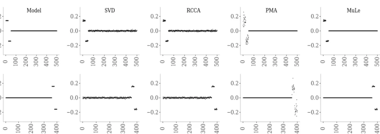
−0.2 0.0 0.2 0 _{100 200 300 400 500} z1 ^ Model −0.2 0.0 0.2 0 _{100 200 300 400 500} SVD −0.2 0.0 0.2 0 _{100 200 300 400 500} RCCA −0.2 0.0 0.2 0 _{100 200 300 400 500} PMA −0.2 0.0 0.2 0 _{100 200 300 400 500} MuLe −0.2 0.0 0.2 0 _{100 200 300 400} z2 ^ −0.2 0.0 0.2 0 _{100 200 300 400} −0.2 0.0 0.2 0 _{100 200 300 400} −0.2 0.0 0.2 0 _{100 200 300 400} −0.2 0.0 0.2 0 _{100 200 300 400}

Figure 1: Comparing performance of different sCCA approaches in recovering the sparsity pattern

and estimating active elements of the canonical directions. TheModel or “true” canonical

directions are plotted in the leftmost plot.

where z1∈R500 and z2∈R400 have the following sparsity patterns,

z1= 1, . . . ,1 | {z } 25 −1, . . . ,₋1 | {z } 25 0, . . . ,0 | {z } 450 z2= 1, . . . ,1 | {z } 25 −1, . . . ,−1 | {z } 25 0, . . . ,0 | {z } 350 (67)

1 ∈R400 and 2 ∈R500 are added Gaussian noise.

1∼ N(0, σ2),∀i= 1, . . .500,

2∼ N(0, σ2),∀i= 1, . . .400,

(68) and

ui ∼ N(0,1),∀i= 1, . . . ,50. (69)

Figure 1comparesMuLe’s performance to the methods mentioned above. The noise amplitude,

σ was set to 0.2, in order to more significantly differentiate between the methods. It is evident

that MuLe successfully identified the underlying sparse model since both the sparsity pattern and

the value of the coefficients were estimated quite accurately, while PMA failed to estimate the

co-efficient sizes accurately. Note here that, our simple cross-validation parameter tuning resulted in

accurate identification of the canonical directions while using the same procedure onPMA resulted

in cardinalities far from the specified model. Hence, the sparsity parameters for the latter method were chosen by trial-and-error to match model’s sparsity pattern.

0.25 0.50 0.75 1.00 0.00 0.25 0.50 0.75 1.00 σ cos ( θ1 ) a 0.25 0.50 0.75 1.00 0.00 0.25 0.50 0.75 1.00 σ cos ( θ2 ) MuLe SVD SVDthr PMA RCCA b

Figure 2: The cosine of the angle between the estimated and true canonical directions, cos(θi) =

|hzˆi,zii|computed for both datasets.

Under the same setting, but varying level of noiseσ, we compute the cosine of the angle between

the estimated, ˆzi, and true,zi, canonical directions,cos(θi) =|hzi,zˆii|fori= 1,2 via the methods

utilized in Figure1. We plotted the results in Figure 2 for both canonical directions; according to

which,MuLeoutperforms other methods, especially the alternating method ofWitten and Tibshirani

(2009), throughout the range of noise amplitude. PMA uniquely shows a lot of volatility in its

solution. The built-in parameter tuning also misspecified the correct sparsity parameters, but providing correct hyperparameters manually also did not help much. Actually, our test shows that

a simple thresholding algorithm like SVDthr outperforms PMA both in terms of support recovery

and direction estimation.

But perhaps the most important piece of information one looks for in high-dimensional multi-view studies is the interpretability of the estimated canonical directions. Therefore, ultimately the decisive criteria in choosing the best approach is determined by how well they uncover the “true” underlying sparsity pattern or simply put, how accurately a model performs variable selection. To this end, variable selection accuracy of each method is plotted against the noise amplitude in Fig.

3 as the fraction of the support of zi, i ∈ {1,2} discovered, here denoted as ηi, vs. the noise

amplitude, σ. As before MuLe performs significantly better than other methods throughout the

noise amplitude range.

7.2 Solution Stability on Data Without Underlying Sparse CCA Model

In the following simulations,X1 andX2are generated by sampling fromN(0pi,Ipi), i∈ {1,2}. The

main purpose of this section is to demonstrate the stability of the solution paths while comparing the quality of the solutions of different algorithms as a function of the cardinality of the canonical loadings. The motivation behind this simulation is that the solution of a stable algorithm must grow more similar to the non-sparse CCA solution. Therefore, while setting the sparsity parameter equal

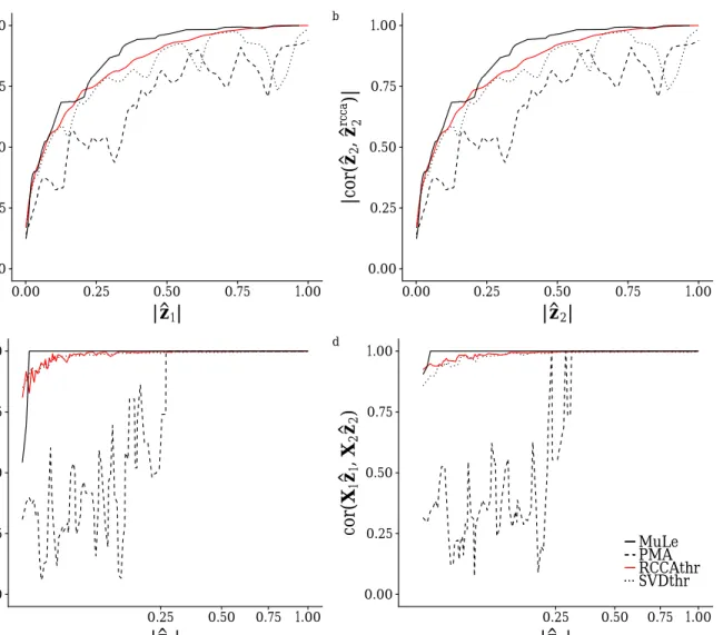
0.00 0.25 0.50 0.75 1.00 0.00 0.25 0.50 0.75 1.00 |z^₁| |cor (z^1 , z^1 rcca )| a 0.00 0.25 0.50 0.75 1.00 0.00 0.25 0.50 0.75 1.00 |z^₂| |cor (z^2 , z^2 rcca )| b 0.00 0.25 0.50 0.75 1.00 0.25 0.50 0.75 1.00 |z^1| cor (X 1 z^1 , X 2 z^2 ) c 0.00 0.25 0.50 0.75 1.00 0.25 0.50 0.75 1.00 |z^2| cor (X 1 z^1 , X 2 z^2 ) MuLe PMA RCCAthr SVDthr d

Figure 3: The correlation between the estimated sparse canonical direction and the direction ob-tained from CCA. (a,b) and the estimated canonical correlation as a function of the cardinality of the estimated direction. (c,d)

to zero for one canonical direction, for an array of sparsity parameters we compute the correlation of the estimated direction with the corresponding direction from the CCA solution, as well as the estimated canonical correlation for the same setting.

The results of the aforementioned simulation is presented in Figure 3. According to our results

MuLe is consistently more correlated with the CCA solution and for (γ1, γ2) = (0,0), it solves the

CCA problem whereas PMAby far does not show the same solution stability. Were columns of Xi

more correlated,PMAand SVDThrwould have resulted in even worse solutions.