Election Forecasting
in a Multiparty System
Bachelor Thesis in Statistics, 15 HEC
Stefan Lindborg (850502-4979), [email protected]
Department of Economics, Fall 2018 Supervisor: Alexander Herbertsson
Acknowledgment
I sincerely want to thank my supervisor, Alexander Herbertsson, at the Department of Economics and Statistics/Center for Finance at the University of Gothenburg. Alexan-der’s inspiration, good advice and suggestions on how to improve this thesis have been invaluable.
Bor˚as, January 29, 2019
Abstract
This bachelor thesis in statistics covers the subject of election forecasting in a multiparty system, using polling data, that is data collected to measure party support, and dynamic linear models (DLMs) with Kalman filtering. In terms of decision-making the outcome of an election can be thought of as an uncertainty. Forecasts of election results can reduce risks for decision-makers and thereby facilitate decision-making. To be able to foresee the outcome of an event can be of use for experts in several different fields, for instance political strategists, financial investors and policy makers. A DLM considers an observable time series to be a linear function of a latent, unobservable series and random disturbance. In the case of election forecasting we can think of the observable series as being polling data, and the underlying series to be true measures of party support. The purpose of using the Kalman filter is then to retrieve the latent series representing true party support. Altogether three different models are explored in the thesis; a Gamma-Normal, a time-invariant and a multivariate time-invariant model. The main difference between the frameworks concerns the variance term in the distribution of the noise terms in the DLM. The models are applied to the Swedish election of 2018, using polling data for the period stretching from September 2014 to September 2018. The polling data is then disregarded for three different time periods; the last month, the last six months and the last twelve months before the election. For those periods, we instead use simulated data which together with the polling data is the basis of our forecasts. We find that the Gamma-Normal model performs slightly better than the two other models, when forecasting the election result one month ahead, while the multivariate time-invariant model is slightly better for the two other time frames. For the one year forecast this model predicts the election result with an average absolute prediction error of 1.28 percentage points for each party. Finally, the forecasting capability of the models are discussed and evaluated in the analysis section of this thesis.
Keywords: Election forecasting, Polling, Multiparty systems, Dynamic Linear Models, DLM, Kalman filtering, Swedish elections
Contents
1 Introduction 4
2 Literature Review 7
3 Theory 11
3.1 Bayes’ theorem and Bayesian analysis . . . 11
3.2 Dynamic linear models . . . 12
3.3 Kalman filtering . . . 15
3.4 Markov chain Monte Carlo methods . . . 17
3.5 Pooling polls . . . 18
4 Methodology and Data 19 4.1 Data . . . 19
4.2 House effects and industry bias . . . 22
4.3 Our algorithm for forecasting the election results . . . 23
4.4 Methodological approach . . . 24
4.5 The Gamma-Normal model . . . 27
4.6 The time-invariant model . . . 29
4.7 The multivariate time-invariant model . . . 29
4.8 Robustness tests . . . 30
4.9 Estimating the model in R . . . 30
5 Results 31 5.1 Estimated house effects . . . 31
5.2 Pooling the polls and estimating latent series . . . 32
5.3 Forecasted results one month before the election . . . 34
5.4 Forecasted results six months before the election . . . 37
5.5 Forecasted results twelve months before the election . . . 39
6 Analysis 43
6.1 Summary of results . . . 43 6.2 Evaluating the over- and underestimated support for some parties . . . . 44 6.3 Limitations regarding model specification . . . 46 6.4 Other problems regarding the model assumptions . . . 48 6.5 The uncertainty of the predictions . . . 49
References 51
Appendix A The multivariate DLM 54
Appendix B Descriptive statistics for each party and polling institute 55
Appendix C Results from the house effect regressions 58
Appendix D Latent series and polls for each party 63
List of Figures
1 Markovian Dependency Structure of Latent Series . . . 13
2 Support for Each Party in Pooled Series, 2014-2018 . . . 21
3 Longer Versus Moving Training Window . . . 26
4 Estimated Latent Series from the Time-Invariant Model . . . 34
List of Tables
1 Descriptive Statistics for the Polling Institutes . . . 202 Descriptive Statistics for the Support for Each Party, 2014-2018 . . . 22
3 Estimated House Effects, 2014-2018 . . . 31
4 The True and Estimated Support on Election Day . . . 33
5 Results from One Month Forecasts, Longer Training Window . . . 35
6 Results from One Month Forecasts, Moving Training Window . . . 36
7 Results from Six Months Forecasts, Longer Training Window . . . 38
8 Results from Six Months Forecasts, Moving Training Window. . . 38
9 Results from Twelve Months Forecasts, Longer Training Window . . . . 40
10 Results from Twelve Months Forecasts, Moving Training Window . . . . 41
1
Introduction
This bachelor thesis in statistics cover the topic of forecasting election results in mul-tiparty systems using a dynamic linear model. The purpose of the study is to develop and explore different models that only use polling data, that is data collected to measure party support, to forecast the Swedish election result in September 2018. A dynamic linear model considers an observable time series to be a function of an underlying unob-servable process and random disturbance (Petris et al., 2009). The forecasting model is based on data from nine different Swedish polling institutes, covering the period between the 2014 and 2018 elections. By the use of Kalman filtering, the unobservable underlying true support for each party is retrieved. Party support is then simulated for different time periods in those series until election day. The simulation is based on a Markov chain Monte Carlo approach, that is a numerical technique to approximate complex integrals, such as conditional probabilities (Petris et al., 2009).
Between 2014 and 2018 the Swedish political landscape went through an extensive trans-formation. As suggested by polling data from before the election, the 2018 election could be thought of as a competition among three major parties of comparable size. Smaller parties like the Liberals, the Green Party and the Christian Democrats seemed to face the risk of loosing all seats in parliament. The election result in September 2018 did however show that the Social Democrats by far remained as the largest party and that all eight parties that were represented in parliament during the period of 2014-18, won seats for the coming term.1 A model with the purpose of forecasting the outcome of the
election needs to capture these trends in the polls, but even so reach conclusions that are close to the actual result.
The research on election forecasting has so far mainly focused on presidential elections in the American two-party system (Sundell & Lewis-Beck, 2014). There are two substantial differences between a presidential election in a two-party system and the Swedish
situa-1The interested reader can notice that the result of the Swedish 2018 election created parliamentary conditions that made it difficult to form a government. It took more than four months until a new prime
tion. Firstly, Swedes do not elect a president, they vote for a party in parliament. In the current situation none of the parties is likely to be able to govern by themselves. This could lead to strategic and tactical aspects that affects the voting decision. Such effects would not be present in a two-party system. Secondly, an American presidential election is dominated by two parties, while eight parties won seats in the Swedish parliament in the 2018 election. These discrepancies lead to methodological challenges limiting the use of so-called structural models.
Election forecasting in Sweden conduced prior to elections has been a rare phenomenon (Sundell & Lewis-Beck, 2014). However, in the scope of the 2014 election several attempts were made to predict the outcome. The most popular prediction model was probably Botten Ada, a ”robot” predicting the election result based on polling data. This website also gained attention of the media (Aftonbladet, 2014; Fokus, 2014). Sundell and Lewis-Beck (2014) used another approach and created a structural model2 that predicted the
result based on economic variables. Walther (2015) made forecasts on the results of the multiparty elections in both Germany and Sweden. Given the increased attention in forecasting election results, it is somewhat surprising that there has not, to our knowledge, been any attempts to forecast the result of the 2018 Swedish election. This thesis could thereby contribute to the research of forecasting Swedish elections by using data from a different time period than prior studies have used.
In terms of decision-making the outcome of an election can be thought of as an un-certainty. Forecasts of election results can reduce risks for decision-makers and thereby facilitate decision-making. To be able to foresee the outcome of an event can be of use for experts in several different fields, for instance political strategists, financial investors and policy makers. In our thesis three different models are evaluated. The first one is a Gamma-Normal model, used in previous similar studies. The second is a time-invariant model, where the support for a party is assumed to be independent of the support for another party. This independency assumption is also included in the Gamma-Normal model. The third model instead assumes that the support for one party is dependent on
2That is a model that uses a regression framework to estimate the support of the incumbent parties using for instance economic variables and underlying political variables.
the support for other parties. This model is referred to as the multivariate time-invariant model. To our knowledge there has not been any attempts to use multivariate models to forecast Swedish election results.
The thesis centers around the following research question:
How well can election outcomes in multiparty systems be forecasted, using polling data and the frameworks of dynamic linear models and Markov chain Monte Carlo techniques? In the thesis we evaluate the performance of election forecasting by DLM models, using the case of the Swedish election in 2018. However, it should be noted that the same techniques could be used to forecast election result in other similar contexts, with for instance a multiparty system. Additionally, DLMs and Kalman filtering could also be used to study subjects unrelated to election forecasting, where there exists an observable process that is a linear function of a latent one. Such examples could be in financial economics, engineering and signal processing.
The rest of the thesis is structured as follows. The upcoming section is devoted to a literature review, which describes previous research on the subject of election forecasting. The following third section covers theoretical aspects of the study, while the fourth section describes the concrete methodology used for answering the research question above. The empirical results are described in the fifth section and finally analyzed in the sixth section.
2
Literature Review
This section presents a literature review, which positions the thesis in relation to previous research conducted on this subject. In the following review different techniques and methods to forecast election are presented and discussed briefly.
The first known attempts to forecast election results took place in the United States during the 1930’s and 1940’s. In 1936 Gallup published its first presidential pre-election survey and in the coming decade the strategy of using so-called bellwether states3 was
tested. However, it took until about 1980 before statistical forecasting models was applied (Lewis-Beck, 2005).
Lewis-Beck and Stegmaier (2014) distinguish between four different approaches to election forecasting; structuralist, aggregators, synthesizers and judges. The structuralists use regression techniques to estimate the support of the incumbent party based on underlying economic and political factors. Theaggregators use polling data, often by pooling several different polls, in order to find a reliable measure on public opinion. The synthesizers combine the methodologies of the structuralists and the aggregators. The most famous model using a synthesizer approach is probably Nate Silver’s FiveThirtyEight model.4
Instead of using quantitative methods, the judges base their forecasts on qualitative assessments of different sources of information. This thesis uses an aggregator approach.
Structural models have traditionally been the common approach to election forecasting (Walther, 2015). Most of these models are based on the assumption that the number of votes for a party in government is a function of political and economical variables. In their most simple forms, these models look like the following (Lewis-Beck, 2005):
Government supportt= Government performancet+ Economic performancet+ Errort
(1)
3That is states where the public opinion would be similar to the nationwide opinion
4The title of the model refer to the number of members of the Electoral Collage that chose the president. Silver became a famous election forecaster when he during the American presidential election in 2012 correctly predicted the outcome of all 50 states (Butterworth, 2014).
Prevalent explanatory variables included in these model have for instance been the popu-larity of the president, left- or right-wing attitudes in the population and the length of the incumbent’s time in office. Economic variables commonly included in the models have been GDP growth, changes in real income and unemployment (Walther, 2015). A famous structural model is theBread and Peace Model in Hibbs (2000), which suggests that the outcome of an American presidential election can be predicted using only two variables; growth in real disposable personal income and the number of American soldiers killed in war. Lewis-Beck and Stegmaier (2000) have reviewed results from studies with struc-tural models conducted on several other countries than the United States. Their results suggest that economic factors play an important role for whether or not an incumbent government can remain in office.
Using a structural model, Sundell and Lewis-Beck (2014) tried to predict the outcome of the 2014 parliament election in Sweden. As dependent variable Sundell and Lewis-Beck use the total vote share for the parties that supported the government, and as explanatory variables GDP growth, inflation and unemployment are used. Their model predicted that the incumbent right-wing government would receive 49.7 percent of the votes, when the actual outcome was only 43.4 percent.
Walther (2015) remarks that structural models are hard to apply in a multiparty context, such as the political landscape in Sweden. Walther mentions three specific reasons for this; the lack of a clear dependent variable, difficulties in attributing economic and political performance to individual parties and the limitations in dealing with new parties. In a two-party system, neglecting the possibility to abstain from voting or to vote blank, the lost votes of the government would go to the opposition party. In a multiparty landscape it is not possible to know how these votes will split among different opposition parties. For instance, differences in policies are likely to affect whether a certain opposition party benefits from a poor economic performance. Walther states that it appears necessary to include polling data to make useful forecasts of the result for every party in a multiparty system.
One early example of how to use polling data to forecast Swedish elections is found in Esaiason and Giljam (1986). In their study they predict the vote share for the Social Democrats and the Left Party. This is done in a regression framework, where this vote share is the dependent variable and the support of these parties in a poll conducted during certain month is the explanatory variable. Esaiason and Giljam reach the conclusion that Sifo’s, a Swedish polling institute, poll in April was the best predictor of the Swedish election results of the six elections between 1970 and 1985.
More modern approaches on how to use polling data to forecast elections involve us-ing dynamic linear models (DLMs). The concept of DLMs is more deeply described in Sections 3.2-3.4, but in short this technique uses pooling of different polls to estimate the underlying support for the parties and simulations to capture the changes in public opinion prior to the election. In addition to describing the DLMs, Walther (2015) also conducts an empirical investigation on whether or not such prediction models can be used to forecast the outcomes of the three Swedish elections between 2006 and 2010 and the three German elections between 2005 and 2013. Walther finds that the average prediction error of a forecast, that is the average difference between the forecasted and the actual election result, conducted one month before the election, is 1.28 percentage points for Sweden and 1.66 percentage points for Germany.
To some extent our study resembles the one in Walther (2015), however there are sub-stantial differences between the approaches. Firstly, we focus only on Sweden and use data from a different period of time than what Walther uses. Our study compares three different types of models, while Walther only covers a model which is similar to our Gamma-Normal model. We evaluate the model’s forecasting abilities on three different time periods; 1 month, 6 months and 12 months before the election. Thereby, we hope to contribute new insights to the field of election forecasting in a Swedish context.
In a master thesis at Link¨oping University, Hurtado Bodell (2016), explores different techniques of pooling polls, using DLM’s. While her techniques is somewhat similar to the ones used in this thesis, the main difference is that she is emphasizing methodologies to pool series while we are focusing more on the simulation phase. However, there is room for future research combining the methodologies for retrieving the latent series capturing true party support, as in Hurtado Bodell, and the simulation techniques used here.
In the context of German elections, Orlowski and Stoetzer (2016) use a DLM framework to forecast party support during election day. In their study different ways of specifying the DLM is evaluated. Their work has been a source of inspiration behind the experiment with the multivariate time-invariant model used in our thesis. Orlowski and Stoetzer also defines a multivariate Gamma-Normal model that can be useful for future research on election forecasting.
3
Theory
This section covers different concepts of theoretical interest for the study conducted in our thesis. Firstly, a short description ofBayesian analysis is provided and thendynamic linear models (DLMs)and different aspects of those are discussed. The process ofKalman filtering is described in Section 3.3, while the section thereafter focuses on Markov chain Monte Carlo methods. Lastly, a review of the concept of pooling polls is presented.
3.1
Bayes’ theorem and Bayesian analysis
Bayesian analysis is based on the principle that all uncertainties should be represented and measured by probabilities (West & Harrison, 1997). From this follows that probabilities are subjective, in the sense that they are a way for the researcher to formalize his or her incomplete information about the event in question (Petris et al., 2009). Bayesian analysis can be thought of as a rational way to update beliefs in light of new information, in order to move from prior beliefs to posterior beliefs. The learning process described above is solved with the use of conditional probabilities. For this Bayes’ theorem is a valuable tool, which in terms of probability distributions and discrete variables Jackman (2009) is described below.
Recall that the conditional probability of A given B, whereP(B)>0 is defined as
P(A|B) = P(B|A)P(A)
P(B) . (2)
The expression sometimes referred to as theBayesian mantra can be derived from Bayes’ theorem: ”the posterior is proportional to the prior times the likelihood” (Jackman, 2009, p. 14). So, here P(A|B) refers to the posterior, P(A) to the prior and P(B|A) to the likelihood.
Bayesian analysis serves the aim of this thesis by giving an approach to how deductions regarding a latent variable can be made using observable data.
3.2
Dynamic linear models
This section will give a brief description of a general univariate DLM, that is used in two out of three models in our thesis. For the multivariate time-invariant model, we instead use a multivariate DLM which is briefly described in Appendix A. The description of the univariate DLM generally follows the steps and the notation mainly in Petris et al. (2009), as well as the discussion in West and Harrison (1997). DLM’s have been used in several other attempts to forecast elections, for instance by Walther (2015), Stoltenberg (2013) and the earlier mentioned Botten-Ada.
Petris et al. (2009) describe DLMs as a class of state-space models. State-space models considers a time series (Yt) to be an incomplete function of a latent and unobserved
process (θt), together with random disturbance. This underlying process is referred to as
the state process or the latent process.
State-space models are based on two assumptions (Petris et al., 2009, p.40):
Assumption 1: The process {θt}, where t = 0,1, ..., n is a Markov chain, which means
that the dynamics ofθt depends on past values only throughθt−1. The probability law of
the processθt is determined by assigning the initial densityp0(θ0) toθ0and the transition
densitiesp(θt|θt−1) of θt conditional on θt−1.
Assumption 2: Conditional on{θt, t= 0,1, ...},Ytis independent from other observations
Ys, fors < t, and depend only on θt. It thereby follows that (Y1, ..., Yn|θ1, ..., θn), for any
n≥1, have a joint conditional density given by Qn
t=1f(yt|θt), wheref(yt|θt) is a density
of Yt given θt. In Bayesian terminology the product
Qn
t=1f(yt|θt) is the likelihood, see
page 11 in this thesis.
With discrete time, as is the case in this thesis, the state-space models are often referred to ashidden Markov models. The Markovian dependency structure is illustrated graphically by Figure 1.
Figure 1: Markovian Dependency Structure of Latent Series
Figure 1, presented in Petris et al. (2009, p. 64), describes how the latent series only depend on its value in the previous time period and the value of the observed series in the current period.
A univariate DLM is characterized as follows. Let tbe an index describing discrete time, Yt an observable time series at timet and Ft a scalar that relates the latent processθt to
the observed one, according to
Yt=Ftθt+vt, vt∼N(0, Vt), (3)
where vt is the time variant disturbance sequence, which follows a normal distribution
with mean zero and variance Vt. In Equation (3) θt is the latent unobservable process,
which relates to its value in the previous time periodθt−1 through the time variant scalar
Gt according to
θt=Gtθt−1+wt wt∼N(0, Wt). (4)
Herewt is the time variant disturbance sequence for the latent process, that is following
a normal distribution with mean zero and variance Wt.
The initial information at timet = 0, which follows a normal distribution, that is
(θ0|D0)∼N(m0, C0) (5)
Equations (3) to (5) are sometimes referred to as the observations equation, the system equation and the initial information (West & Harrison, 1997).
The random walk with noise model is the simplest form of DLM and refers to a model where the conditional expectation of a time series att, given its previous values, is equal to the value of the series at t−1, that is E[Yt|Yt−1, Yt−2, ...] = Yt−1 (Stock & Watson,
2015). The general DLM, defined by Equations (3) to (5), can be transformed into a random walk with noise model, by setting Ft = Gt = 1 which also implies that the
scalars Ft and Gt are assumed to be time invariant. After changing the notation, the
underlying latent processθtis now denoted byµt, which leads to the following equations,
describing the model used in this thesis (West & Harrison, 1997)
Yt=µt+vt vt∼N(0, Vt) (6)
µt=µt−1+wt wt∼N(0, Wt) (7)
(µ0|D0)∼N(m0, C0), (8)
where Vt, Wt and C0 are the same as in Equations (3) to (5).
The random walk model above, defined by Equations (6)-(8), is often used for short-term forecasting (West & Harrison, 1997). This stochastic process µt has an important
property, the conditional expected value of the forecastksteps ahead from time tis equal to the value of the latent process at t, that is
E[Yt+k|µt] =E[µt+k|µt] =µt, (9)
which follows from Equations (6) and (7), see also p. 34 in West and Harrison (1997).
If we define the forecast function ft(k) asE[Yt+k|Dt], where Dt refers to the information
available at time t, that isDt=y0, y1, ..., yt where yt is the realization ofYt, then
This means that the forecast function, ft(k) is constant in the sense that it does not
depend on k. So, no matter the number of steps ahead the forecast ft(k) for a given
information set,Dt, remains constant at mt where mt =µt−1 (West & Harrison, 1997).
3.3
Kalman filtering
Kalman filtering refers to a recursive procedure to make inferences of a unobservable latent processµt, through the use of Bayes’ theorem. The application of Kalman filtering
has been common in engineering, for instance for signal processing. Bayes’ theorem states that the posterior distribution of µt is proportional to the product of the likelihood and
the prior distribution ofµt. The prior distribution ofµtrefers to its distribution when the
value of Yt is not known, while the posterior distribution of µt refers to its distribution
when new information is available (recall Equation (2) and see Section 3.1 for a deeper description of Bayes’ theorem). Formally this can be expressed as
p(µt|Dt)∝p(Yt|µt, Dt−1)×p(µt|Dt−1), (11)
where Dt as earlier refers to the information available at time t and ∝ meaning ”linear
proportional to”.
The inference is made in two steps; first prior to observingYtand then after observing Yt.
Prior to observingYtthe best guess of µt is simply the relationship captured in Equation
(4). When Yt is observed, Equation (11) can be used to calculate the posterior p(µt|Dt).
This will be done using the forecast erroret which is defined aset =Yt−ft=Yt−mt−1
and possible to calculate after observing Yt. Again, using Bayes’ theorem we can state
that
p(µt|Yt, Dt) =p(µt|et, Dt−1)∝p(et|µt, Dt−1)×p(µt|Dt−1) (12)
p(µt|Yt, Dt−1) =
p(µt|et, Dt−1)×p(µt|Dt−1) R
allµtp(µt|et, Dt−1)dµt
. (13)
The description above of Kalman filtering is based on Meinhold and Singpurwalla (1983).
The Kalman filter results in a filtering densityp(µt|Yt, Dt), which follows a normal
distri-bution. In the case of a random walk with noise model, the parameters are the following:
(µt|Dt)∼N(mt, Ct), (14)
where mt =mt−1+Ktet and Ct =KtVt. Here Kt is defined as Kt = CtC−t1−+1W+Wt+tVt, where
Vt and Wtis the same as in Equations (6) and (7). The variable et can be understood as
the forecast error and is defined as et=Yt−ft=Yt−mt−1.
By using the definition of the variables in Equation (14) we can think ofmtas a weighted
average of Yt and mt−1, since we have mt = (1−Kt)mt−1 +KtYt. Also, Kt can be
understood as an adaptive coefficient between 0 and 1 (Petris et al., 2009). Thereby it is clear that the relationship between the latent and the observed processes are affected by the values of Vt and Wt. This also means that the predictive capability of the model will
depend on those as well.
The Kalman filter returns the one-step ahead forecast for the observed process, as below (West & Harrison, 1997):
(Yt+1|Dt)∼N(ft, Qt), (15)
3.4
Markov chain Monte Carlo methods
In many practical applications of DLMs every component of the model is seldom known. In the perspective of Bayesian analysis these unknown parameters are considered to be random variables. This means that it is necessary to find the joint conditional distribu-tion of the latent series and its forecasted values, as well as the unknown parameters. This usually leads to expressions that cannot be solved analytically, instead a numerical approach is necessary. This usually involves an application of Monte Carlo techniques to Markov Chains, often known asMarkov chain Monte Carlo (MCMC) methods (Petris et al., 2009).
For the case of this thesis, µj,t is the quantity of interest, describing the true support for
partyj at timet. Now assume that it has a posterior distributionp(µj,t|Dj,t−1, Yj,t). Also
assume thatµj,T is the true support for partyj on the day of the election (that ist=T).
We are interested in forecasting the quantity µj,T using direct posterior sampling from
the posterior distribution defined above. Further, assume that g(µj,t) is some arbitrary
function of µj,t. Let m denote the number of Monte Carlo iterations, as m → ∞ the
following holds based on the law of large numbers and conditions that are generally fulfilled (West & Harrison, 1997)
E[g(µj,t)] = Z g(s)p(s|Dj,t−1, Yj,t)ds p → 1 m m X i=1 g(µj,t), (16)
where →p means convergence in probability, see for instance Wackerly et al. (2008, p. 448-454).
3.5
Pooling polls
To make predictions about the future based on a latent variable one needs to have a good estimate of its current value. Only on election days we get to have true measures of party support, here denoted by θ. Vote shares in upcoming elections are unknown at forehand and is a result, not only of events on the day of the election but from flows that take place between elections. That is, we have missing values for true party support all other days than election days. However, we do have polls that are inaccurate, and probably at least to some extent, erroneous. This illustrates the purpose of using DLMs to estimate and forecast party support (Stolenberg, 2013).
Jackman (2005) lists three potential problems with making inferences about public opin-ion based on individual polls; imprecise estimates due to sampling error, bias induced by the methods and the fact that public opinion is likely to change between the time of the poll and the election. Jackman also concludes that the sample size of many polls are too small to detect small changes in party support with certainty.
Jackman further describes how pooling of polls can increase the precision of the estimates, that is reduce the standard deviation. Consider two polls, A and B, estimating a true quantity α. The estimate from poll A will follow a normal distribution with mean ˆαA
and standard deviation sA =
p
ˆ
αA(1−αˆA)/nA, where nA is the sample size of poll A.
The same goes for the estimate ˆαB and sB. If we pool A and B we will have a precision
weighted average of both polls
ˆ αAB =
pAαˆA+pBαˆB
pA+pB
, (17)
where pA is the precision of pollA and defined as 1/s2A and pB is the precision of poll B
defined analogously. The standard deviation for the pooled poll issAB =
p
1/(pA+pB),
4
Methodology and Data
This section serves the purpose of describing the methodological approach in the thesis and the data used for performing the study. Section 4.1 covers the data, how it is processed and also presents some descriptive statistics. The second subsection is devoted to giving an insight of how the house effects are calculated. The term house effects refers to ”bias induced by methodological procedures specific to each polling organisation” (Jackman, 2005, p. 500). Section 4.2 also describes how the bias created by differences in methodology between polling institutes distinguish from industry bias, while Section 4.3 gives an overall description of the methodological approach. Thereafter, the subsections define the specific Gamma-Normal model, the time-invariant model and the multivariate time-invariant model. The two final subsections describes robustness checks and the data programming.
4.1
Data
The empirical examination is based on a compilation of Swedish polls from Magnusson (2018). The time period of interest is defined as the period between the 15th of September in 2014 and the 8th of September in 2018, that is the period between the 2014 and 2018 elections. However, the data set provided by Magnusson goes back to 1998 and stretches to the present. For the time period of interest the material covers polls from nine institutes;Demoskop,Inizio,Ipsos,Novus,SCB,Sentio,Sifo,Skop andYouGov. All together the compilation in early October 2018 contained 1522 different polls. 384 polls remain after selecting only those made during the time period of interest. Polls where the institute, collecting period or sample size are unknown are disregarded. By this the number of polls decrease to 375.
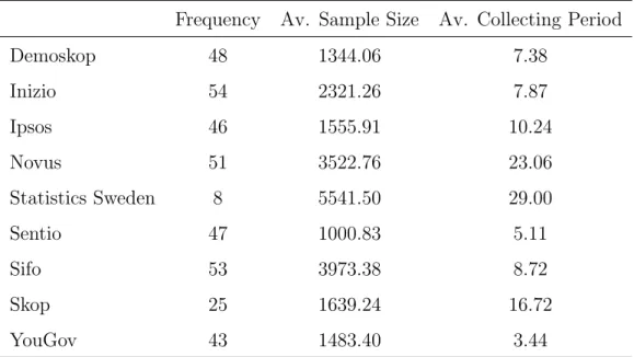
Table 1 below presents descriptive statistics for the polls from the nine different institutes. As can be seen from Table 1, the frequencies of the polls in the data material differs. The polls from Statistics Sweden stand out, since they are only done twice a year. On the other hand these polls have large sample size and a longer collecting period (measured
in days). The most frequent poll is the Inizio poll, which have been performed 54 times during the period of interest.
Table 1: Descriptive Statistics for the Polling Institutes
Frequency Av. Sample Size Av. Collecting Period
Demoskop 48 1344.06 7.38 Inizio 54 2321.26 7.87 Ipsos 46 1555.91 10.24 Novus 51 3522.76 23.06 Statistics Sweden 8 5541.50 29.00 Sentio 47 1000.83 5.11 Sifo 53 3973.38 8.72 Skop 25 1639.24 16.72 YouGov 43 1483.40 3.44
The table describes the polls from the nine polling institutes between September 2014 and September 2018. It covers the number of polls from each institute, their average sample size and average data collecting period (Magnusson, 2018).
In Appendix B, boxplots illustrating the average support and its dispersion for each party and house are presented.
From the polls of the nine different institutes displayed in Table 1 we construct one pooled series describing the evolution of each party’s support during the period. By assuming that the number of interviews have been the same for each day during the collecting period, each poll is split into daily data. This means that a certain day can be covered by several different polls. To make one merged time series Yj,t for each party, it is necessary
to combine the information in the different polls. We weigh the polls by sample size and calculate an average describing the support for each party on a given day. Before this, the house effects are taken into account. The new merged series of polling data have 1369 observations for eight parties, which means that 94 percent of the 1454 days between
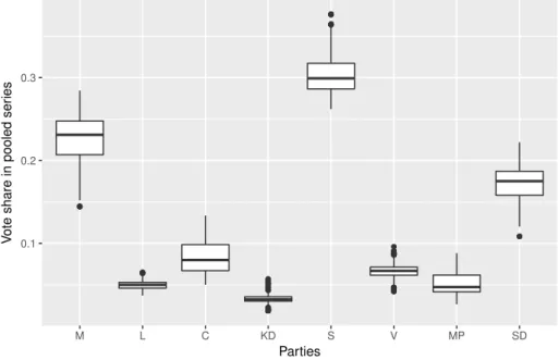
the elections are covered. Table 2 and Figure 2 below, present descriptive statistics for this merged series. Figure 2 contains boxplots that describe the mean and variance of the support for each party in the pooled series, and as can be seen from this figure, the support for some parties have varied substantially during the period of interest. For other parties – especially the Liberals, the Christian Democrats and the Left Party – the support has been more or less constant during the time period.
Figure 2: Support for Each Party in Pooled Series, 2014-2018
0.1 0.2 0.3 M L C KD S V MP SD Parties V
ote share in pooled ser
ies
Figure 2 contains boxplots that for each party illustrate the mean and the variance of its support during the period of September 2014 to September 2018.
Table 2 describes the pattern illustrated by Figure 2 more precisely. The table presents the average support for each party, its standard deviation and the minimum and maximum support.
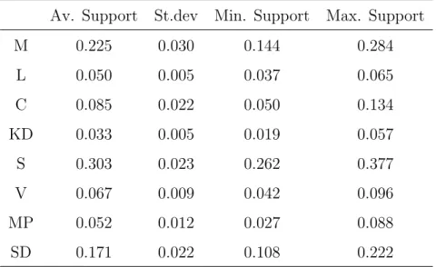
Table 2: Descriptive Statistics for the Support for Each Party, 2014-2018
Av. Support St.dev Min. Support Max. Support
M 0.225 0.030 0.144 0.284 L 0.050 0.005 0.037 0.065 C 0.085 0.022 0.050 0.134 KD 0.033 0.005 0.019 0.057 S 0.303 0.023 0.262 0.377 V 0.067 0.009 0.042 0.096 MP 0.052 0.012 0.027 0.088 SD 0.171 0.022 0.108 0.222
Descriptive statistics for the support of each party in the pooled series, stretching from September 2014 to September 2019.
4.2
House effects and industry bias
Jackman (2005) states that pooling the polls lead to better precision, under the criteria that the polls are unbiased. There are several reasons for why the results of different polls can be biased. For example because of differences in interviewing methods, sampling, weighting procedures and how questions are formulated. This could cause the estimated support for certain parties to be systematically wrong.
To estimate house effect it is necessary to choose one of the institutes as a benchmark, which polls are thereby considered to be unbiased. In this study the polls from Statis-tics Sweden, that is the Swedish governmental agency for official statistics, are used as a benchmark. The argument for choosing this institute is that it has a conservative methodology and a much larger sample size than other institutes. The house effects are modelled for each party using a linear regression, where binary variables for all institutes except for the benchmark, are used as independent variables. The regression models can be written as:
Yj,i =α+Xiβ+εi (18)
Here Yj,i represents the support for party j in poll i, X is a vector of binary variables
indicating which house that made polliand the subscriptirefers to the poll in question. If the coefficient for one of the dummy variables is statistically significant at least on a 5 percent level, this house is considered to systematically either under- or overestimating the support for the party in question (Fisher et al., 2011; Walther, 2015). The house effects for each party and institute are presented in Section 5.1. These are then transformed and used as weights when the polls are pooled.
Another type of bias than house effects is industry bias. This term refers to systematic errors in the industry as a whole, that is errors that all polling institutes suffers from. This type of bias could be found, for instance if the sum of all house effects is not equal to zero (Fisher et al., 2011). Industry bias is not taken into account in the filtering process and can thereby be a potential reason for why forecasts can be less precise compared to the actual outcome.
4.3
Our algorithm for forecasting the election results
Before going into detail on the methodological approach we outline the stepwise algorithm used in our study. The purpose of describing our algorithm for election forecasting is to facilitate the understanding of the overall methodology used in the thesis.
1. Aggregate the polls into one pooled series of daily measures of polled party support, following the procedure described in Section 4.1.
2. Define the DLM by first assuming that party support follows a random walk with noise framework, which means that Equations (6) to (8) form the basis of the model. Then specify the model further using the different frameworks described in Sections 4.5 to 4.7.
3. Use Kalman filtering to retrieve the latent series describing true party support at a given time, with the procedure described in Section 3.3.
4. Use the filtered series to simulate the change in party support from the stop date, that is the last day with polling data, until the election day, using a MCMC approach such that the predictive density at time tretrieved by the Kalman filter is used for simulating polling data for time t+ 1. By doing this the filtering process is updated. This goes on untilt =T.
5. The forecast is then compared to the actual election result and the predictive capability of the model is evaluated, both in terms of bias and variance.
4.4
Methodological approach
Given the definition of the algorithm in the previous subsection, this section focuses on the methodological approach in more detail. In two out of three DLM models, the Gamma-Normal and the time-invariant models, support for party j is assumed to be independent of the support for the other parties. Then Yj,t are eight independent time
series. In the third model, the multivariate time-invariant model, the series is instead a vector with dimension 8×1, denoted Yt. In this aspect, the unobserved latent series
µj,t and µt have the same functioning as the observed series. For all three models, the
underlying model assumption is that party support can be modelled using a random walk with noise model, as specified in Equations (6), (7) and (8).
The difference between the Gamma-Normal model and the time-invariant model refers to the assumptions onVj,t andWj,t in Equations (6) to (8). The behavior ofVj,t andWj,t
is crucial for the forecasts. In the Gamma-Normal modelVj,t is updated using a binomial
approximation of the variance, while Wj,t is assumed to follow a gamma distribution
with certain shape and rate parameters. In the time-invariant model Vj,t = Vj and is
approximated with the sample variance of the series Yj,t and Wj,t =Wj is approximated
using the sample variance of the latent series based on polling data µj,t. The difference
Σw, the covariance matrices, are used instead of the variancesVj andWj in the later one.
These matrices are calculated in the same way as the variance terms in the time-invariant model.
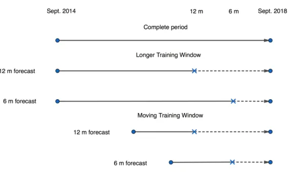
Moreover, forecasts are done for three different time-periods; one month, six months and twelve months before the election. Naturally the uncertainty of the forecast should be larger for longer periods of simulations. The last day with polling data is referred to as the stop date. In Figure 3, the stop date is illustrated by the crosses. Each model is first estimated using a longer training window, that is using data for the complete period from September 2014 until the stop date, as shown by the second and third line of Figure 3, where the period with polling data is the solid line and the period with simulated data has a dashed line. Then we compare the results to a forecast where instead a moving training window is used, and this approach uses only polling data that stretches back one year in time from the stop date. This is illustrated by the fourth and fifth line of Figure 3. As can be seen in Figure 3, the moving training window is based on less data, and the period where the data is collected from differs between the time frames of the forecast.
To clarify the difference between the longer and the moving training windows we will present two examples. For both windows, the 12 month forecasts have a stop date in September 9 2017 and both use one year of simulated data. However, in the longer training window this forecast is based on data stretching back to September 2014 while in the moving training window the underlying data only goes back to September 2016. Essentially the same holds for the 6 months forecasts. Both windows have a stop date in March 9 2018 and uses half a year of simulated data. In the longer training window the underlying data still goes back to September 2014, but in the moving training window we use polling data from March 2017 until the stop date.
Figure 3: Longer Versus Moving Training Window
Difference between the longer training window and the moving training window. While the longer training window uses data from September 2014 to the stop date, the moving training window uses data for a one-year-period that stretches one year back from the stop date. The solid lines are periods with polling data, the dashed lines are periods with simulated data and the crosses are the stop dates.
The forecasting procedure is repeated 10,000 times using a MCMC approach. The sim-ulation for each iteration is done sequentially. First data points for the series Yj,t are
simulated from the posterior distributions retrieved from the Kalman filtering. Then the Kalman filters are updated and new data points are simulated. This procedure continues until the day of the election. For the Gamma-Normal model it is necessary to update the time invariant variances for each day. The resulting forecast of the election result is then used for calculating an average prediction and a 95 percent (empirical) confidence interval. These intervals are then compared to the election results for each party, with the purpose of evaluating the capability of the model. The main instrument for evaluating the precision of each forecast is referred to as theaverage prediction error, and is defined according to
Average prediction error = 1 8 8 X j=1 |µ∗j,T −µ¯ˆj,T |, (19)
where µ∗j,T is the election result in September 2018 and ¯µˆj,T is the point estimate of the
forecasted result for party j, obtained via the MCMC-approach. Finally, the robustness of the model is examined using different assumptions on Vj,t and Wj,t.
4.5
The Gamma-Normal model
As discussed in Stoltenberg (2013), the Gamma-Normal model is based on strong and unrealistic assumptions. However, it serves the purpose of facilitating the modelling. The underlying assumption behind how Vj,t is defined in this model, see Equation (24),
is that the data generating process can be described as a series of independent Bernoulli experiments, where each respondent in the polling institute’s survey can state that they will vote for a certain party or that they will not. This means that the series of polling data must be considered as eight independent series, one for each party. This is a theoretically unrealistic assumption, that in practice could lead to that the sum of the forecasted support for all parties exceed one. In reality this would not, of course, be feasible. Here that risk is handled by normalizing the simulated support for all parties.
The basis for the Gamma-Normal model is eight univariate DLMs, based on the following equations:
Yj,t=µj,t+vj,t vj,t ∼N(0, Vj,t) (20)
µj,t =µj,t−1+wj,t wt∼N(0, Wj,t) (21)
(µj,t|Dj,0)∼N(mj,0, Cj,0), (22)
where j = 1, ...,8 is an index describing the eight parties and t = 1, ...,1454 is a time index, describing the number of days between the 2014 and 2018 elections. The one-step-ahead forecast for the observed process Yj,t would then be
(Yj,t|Dj,t−1)∼N(fj,t, Qj,t), (23)
where fj,t = mj,t−1 and Qt = Cj,t−1 +Wj,t+Vj,t. The terms Vj,t and Wj,t are unknown.
First, Vj,t is calculated using the formula for calculating the variance in a binomial
dis-tribution. Such a binomial approximation relates to the fact that a binomial distribution consists of a sum of Bernoulli distributions, so that
Vj,t =
yj,t(1−yj,t)
nt
, (24)
whereyj,t refers to the polled support for partyj at timet andntrefers to the number of
interviews made on day t. For the days between the last day with polling data and the election day, nt is simulated and is assumed to be nt ∼U nif(a, b), wherea and b is the
values of the 25th and the 75th percentile of the actual data for n.
SinceWj,tis unobserved we cannot use it directly. Instead our study follows the suggestion
by West and Harrison (1997) and uses the so-called precision, φj,t, defined as φj,t = W12
j,t. Also the precision is unknown, but it is assumed that it follows a gamma distribution with parameters a and b, φj,t ∼ Gamma(a, b).5 Here the following definitions are used
a= 1 and b = 2000, so that the expected daily volatility of the latent series for a certain party is 0.005 percentage points. Stoltenberg (2013) uses b = 5000 for the Norwegian Labour party.
In order to simplify the model we have chosen to treataandbas being equal for all parties and time-periods. In future studies it could be relevant to alter these parameters based on the volatility of the support for different parties and time-periods. This is discussed more in Section 6.5.
4.6
The time-invariant model
The second type of model in this study is referred to as the the time-invariant model. Also here the time series for each party is assumed to be independent of the ones from other parties and the basis of the model is the eight DLMs described by Equations (20), (21) and (22). The only difference between the two models is that we haveVj,t=Vj and
Wj,t =Wj.
To estimate the time-invariant model it is necessary to make assumptions on howVj and
Wj behave. Here it is assumed that Vj = V ar(yj), that is it is assumed to be equal to
the sample variance of the polling data for party j for the period of interest. The term Wj is assumed to be proportional to Vj with a factor of 0.5, so Wj = 0.5·Vj. Here the
0.5 factor can be thought of as a discount factor, which it is referred to in both West and Harrison (1997) and Petris et al. (2009).
4.7
The multivariate time-invariant model
In the multivariate time-invariant model the support for party j is instead assumed to be dependent on the support for the other parties. This is a more realistic assumption, since party support is a zero-sum game. If the support for one party increases, at least one other party must lose support.
The dependency structure is captured by the fact that in this case V and W are invariant covariance matrices, estimated from the data in the same way as the time-invariant variances in the model described in Section 4.6. The empirical covariances are used as estimates, and these are assumed to be time-invariant. The relationship between matrix V and matrix W are defined in the same way as in the time-invariant model, such that W = 0.5·V.
4.8
Robustness tests
West and Harrison (1997) describes how the forecast depends on Vj,t and Wj,t. The
purpose of our first robustness check is to examine how the choice of the rate parameter in the gamma distribution of the precision, φj,t ∼ Gamma(a, b), affects the model’s
forecasting ability. The choice of b = 2000 as a general starting point is to a high degree arbitrary, therefore it is interesting to repeat the simulation using other values of this parameter. Here it will be examined whether or not the results will be similar forb = 500 and b = 5000. The robustness check is based on the Gamma-Normal model, with 6 months between the end of polling data and election day and a moving training window. The reason for why only the six months time frame is chosen for the robustness tests is due to the long time it takes to simulate the data.
The second robustness check examines whether the results change significantly in the time-invariant models when the discount factor is set to 0.25 and 0.75, instead of 0.5. The basis also for the second robustness check is the 6 months variant with a moving training window. This process is repeated for both the time-invariant model and the multivariate time-invariant model.
In addition, using the longer and the moving training window can be considered a ro-bustness check that investigates how sensitive the models are for different amounts of data.
4.9
Estimating the model in
R
For estimating the model in R several functions from the ”DLM” package, described in Petris (2010), has been invaluable. Our R program uses for example the function dlm for estabilsiing the DLM models for each party and dlmF ilter for the Kalman filtering, but thre rest of our R-code has been implemented by us from scratch, in particular the part for simulating the change in party support between the stop date and the day of the election.
5
Results
This section consists of six subsections. The first two describes the estimated house effects and the estimated latent series for true party support. Sections 5.3 to 5.5 are devoted to the results from the three different time frames, that is one, six or twelve months before thee election, of the forecast model, while Section 5.6 presents the results of the robustness tests.
5.1
Estimated house effects
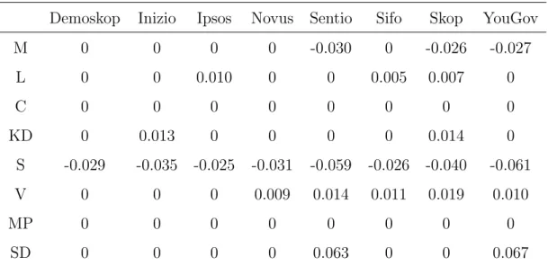
As described in Section 4.1 house effects are biases that are created by the methodologies used by different polling institutes. This could lead to a systematic over- or underestimate of the support for a certain party. In Table 3 below, the estimated house effects for each party and polling institutes are displayed, that is the vector β in Equation (18). The table only consists of significant estimates at the 5 percet level, see Tables 12 to 19 in Appendix C.
Table 3: Estimated House Effects, 2014-2018
Demoskop Inizio Ipsos Novus Sentio Sifo Skop YouGov
M 0 0 0 0 -0.030 0 -0.026 -0.027 L 0 0 0.010 0 0 0.005 0.007 0 C 0 0 0 0 0 0 0 0 KD 0 0.013 0 0 0 0 0.014 0 S -0.029 -0.035 -0.025 -0.031 -0.059 -0.026 -0.040 -0.061 V 0 0 0 0.009 0.014 0.011 0.019 0.010 MP 0 0 0 0 0 0 0 0 SD 0 0 0 0 0.063 0 0 0.067
Estimated house effects for each party and polling institute. The full results of the regressions can be found in Appendix C.
A positive estimate means that the polling institute in question systematically overesti-mates the support for a certain party, while a negative estimate means that the support is systematically underestimated. The magnitude of the numbers refers to the average difference in percentage points from the estimate made by Statistics Sweden. The esti-mated house effects are then used to weigh the polls for each party before all polling data is merged into one series.
The negative house effects for the Social Democrats in all polling institutes is troubling, since it could suggest that Statistics Sweden overestimated the support for the party rather than that all other houses underestimated their support. This is also a comment that sometimes is made from political journalists and commentators, see for instance Expressen (2014). If so, the choice of Statistics Sweden as a benchmark would not be appropriate. This question is further discussed in the analysis of this thesis.
In earlier election campaigns the Sweden Democrats have been considered to be a party that is hard to poll. The estimated house effects in Table 3 shows that, compared to Statistics Sweden, two polling institutes; Sentio and YouGov significantly overestimated the support for this party. Both these institutes use self-recruiting web panels and Sentio does not reveal their methodologies (Sundell, 2015). The same institutes have large negative house effects for the Social Democrats.
No significant house effect at all can be found for the Centre Party and the Green Party. For the other parties the estimated house effects are small and often not significant.
5.2
Pooling the polls and estimating latent series
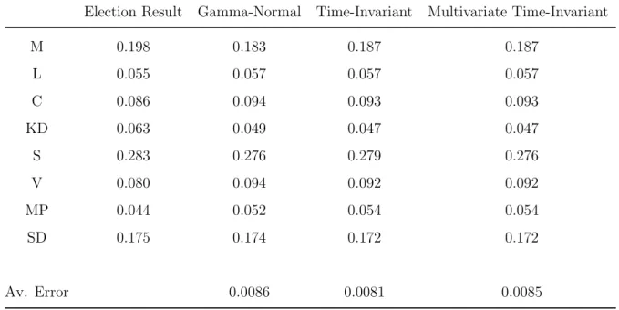
Table 4 presents the result of the estimated latent-series. Here, simulated data is not used, instead the Kalman filtering runs through the complete series of pooled polls for the whole period between September 2014 and September 2018. The pooling methodology in our thesis can be evaluated by comparing the estimates for the latent series on election day, which in turn should describe the true underlying party support that day, to the election result in September 2018. The election results are compiled from (Valmyndigheten, 2018).
For all three models the result is on average deviating with 0.8 percentage points from the election result.
Table 4: The True and Estimated Support on Election Day
Election Result Gamma-Normal Time-Invariant Multivariate Time-Invariant
M 0.198 0.183 0.187 0.187 L 0.055 0.057 0.057 0.057 C 0.086 0.094 0.093 0.093 KD 0.063 0.049 0.047 0.047 S 0.283 0.276 0.279 0.276 V 0.080 0.094 0.092 0.092 MP 0.044 0.052 0.054 0.054 SD 0.175 0.174 0.172 0.172 Av. Error 0.0086 0.0081 0.0085
The table contains support for each party in the 2018 election and also the support on election day in the estimated latent series. The latent series are estimated for all three models. The average error is the average distance between the estimate and the election result, see Equation (19).
Figure 4 illustrates the latent series for all parties from the time-invariant model only, but as can be seen from Table 4 the endpoints of all three models do not deviate substantially from each other. The estimated latent series for each party resembles the pattern in the boxplots of Figure 2. Series for the parties where the boxes illustrate a larger spread is more volatile. This is important for the consistency of the results. Appendix D includes figures that for each party relates this series to the polling data. The same appendix also contains estimated latent series for the Gamma-Normal and the multivariate time-invariant model.
Figure 4: Estimated Latent Series from the Time-Invariant Model 0.1 0.2 0.3 2015 2016 2017 2018 Time V ote share C KD L M MP S SD V
The figure presents the estimated latent series for each party, using the time-invariant model. Appendix D includes both figures that for each party relates this series to the polls and the estimated latent series for the Gamma-Normal and the multivariate time-invariant model.
5.3
Forecasted results one month before the election
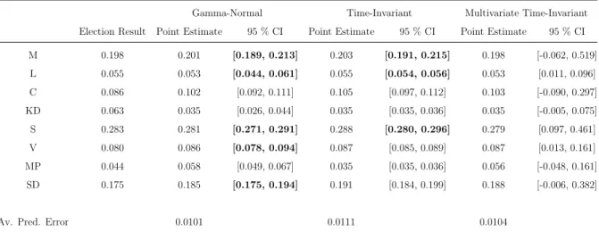
Table 5 below presents the result of the forecast conducted one month before the election for all three models, using the longer training window. The table shows both point estimates and the interval in which 95 percent of the election forecasts are found.
When it comes to the point estimates, there are small differences between the three mod-els. In general all models predict the result of the Moderates, the Liberals and the Social Democrats well. On the other hand, all three models have problems forecasting the result for the Christian Democrats, which are underestimated, and the Centre Party, which are
overestimated. In Sweden the right-wing parties, that is the Moderates, Liberals, Centre Party and Christian Democrats, have formed a pre-election coalition, ”the Alliance”. The red-green parties, that is the Social Democrats, the Left Party and the Green Party, have had a similar cooperation before the election. On a party alliance level the best model underestimates the support for the Alliance with -1.2 percentage points and overestimates the support for the Red-Green Party with 1.8 percentage point.
Table 5: Results from One Month Forecasts, Longer Training Window
Gamma-Normal Time-Invariant Multivariate Time-Invariant
Election Result Point Estimate 95 % CI Point Estimate 95 % CI Point Estimate 95 % CI
M 0.198 0.201 [0.189, 0.213] 0.203 [0.191, 0.215] 0.198 [-0.062, 0.519] L 0.055 0.053 [0.044, 0.061] 0.055 [0.054, 0.056] 0.053 [0.011, 0.096] C 0.086 0.102 [0.092, 0.111] 0.105 [0.097, 0.112] 0.103 [-0.090, 0.297] KD 0.063 0.035 [0.026, 0.044] 0.035 [0.035, 0.036] 0.035 [-0.005, 0.075] S 0.283 0.281 [0.271, 0.291] 0.288 [0.280, 0.296] 0.279 [0.097, 0.461] V 0.080 0.086 [0.078, 0.094] 0.087 [0.085, 0.089] 0.087 [0.013, 0.161] MP 0.044 0.058 [0.049, 0.067] 0.035 [0.035, 0.036] 0.056 [-0.048, 0.161] SD 0.175 0.185 [0.175, 0.194] 0.191 [0.184, 0.199] 0.188 [-0.006, 0.382]
Av. Pred. Error 0.0101 0.0111 0.0104
The results from the one month forecasts for the three models, when a longer training window is used. The bold intervals are those intervals that capture the true election results in the Gamma-Normal and Time-Invariant models.
The average prediction error, as defined by Equation (19), is similar for all three models. The Gamma-Normal model performs slightly better than the others.
The width of the confidence intervals can be considered to capture the uncertainty of the forecast. The uncertainty is by far the largest in the multivariate time-invariant model. Some election forecasts in this model are actually negative, which of course is unreasonable. The time-invariant model has a slight lower uncertainty than the Gamma-Normal model. Therefore the choice between this model and the other two can to some extent be thought of as a choice capturing the bias-variance trade-off which is common in statistics.
For illustrative purposes we have in Tables 5 to 10 displayed the intervals covering the true election results in the Gamma-Normal and the time-invariant models in bold. This is not done for the multivariate time-invariant model because of its unrealistic intervals. For the Gamma-Normal model five out of eight intervals capture the true election result in September 2018, and for the time-invariant model three out of eight forecasts cover the true result.
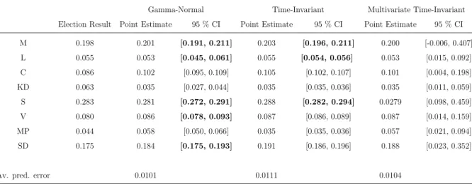
When a moving training window is used the point estimates are identical for the Gamma-Normal and the time-invariant models, and the results are presented in Table 6. For the multivariate time-invariant model there are some small differences, although the aver-age prediction error remains the same. On the other hand, the moving training window results in smaller uncertainties for all models. The largest improvement is for the multi-variate time-invariant model, which however still remains to be the model with the largest uncertainty.
Table 6: Results from One Month Forecasts, Moving Training Window
Gamma-Normal Time-Invariant Multivariate Time-Invariant
Election Result Point Estimate 95 % CI Point Estimate 95 % CI Point Estimate 95 % CI
M 0.198 0.201 [0.191, 0.211] 0.203 [0.196, 0.211] 0.200 [-0.006, 0.407] L 0.055 0.053 [0.045, 0.061] 0.055 [0.054, 0.056] 0.053 [0.015, 0.092] C 0.086 0.102 [0.095, 0.109] 0.105 [0.102, 0.107] 0.101 [0.004, 0.198] KD 0.063 0.035 [0.027, 0.044] 0.035 [0.035, 0.036] 0.035 [0.011, 0.059] S 0.283 0.281 [0.272, 0.291] 0.288 [0.282, 0.294] 0.0279 [0.098, 0.459] V 0.080 0.086 [0.078, 0.093] 0.087 [0.086, 0.089] 0.087 [0.014, 0.159] MP 0.044 0.058 [0.050, 0.066] 0.035 [0.035, 0.036] 0.057 [0.021, 0.094] SD 0.175 0.184 [0.175, 0.193] 0.191 [0.186, 0.196] 0.188 [0.023, 0.352]
Av. pred. error 0.0101 0.0111 0.0104
The table presents the results from the one month forecasts for the three models, when a moving training window is used. The bold intervals are those intervals that capture the true election results in the Gamma-Normal and Time-Invariant models.
5.4
Forecasted results six months before the election
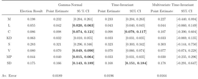
Table 7 presents the result of the forecasts conducted six months before the election, when the longer training window is applied. Overall the average prediction error increases substantially compared to the forecast one month before of the election in September 2018. For the Gamma-Normal and time-invariant models the average prediction error is close to 2 percentage points, while it is substantially better for the multivariate time-invariant model. T average prediction error is for the latter model only about 1.6 percentage points. This is mainly driven by more realistic predictions for the Centre Party, the Social Democrats, the Left Party and the Sweden Democrats. Except for these results, the individual forecasts are quite similar between the models.
On a party alliance level the best model, the multivariate time-invariant model with a moving training window, perform even better than the best model in the one month forecast. For the best six months model the difference between the election result for the right-wing alliance is only 0.6 percentage points and for the red-green parties only 1.3 percentage points. Thus, both blocs are overestimated.
The uncertainty, as described by the width of the confidence intervals, has increased compared to the one month forecasts. This phenomenon is illustrated by the fact that the intervals are wider here. The problem of the unrealistically large variance for the multivariate time-invariant model remains, and is further exacerbated. As earlier the bold intervals in the Gamma-Normal and time-invariant models cover the true election result. For the Gamma-Normal model five out of eight predictions cover the true election result. This is an identical result compared to the forecast one month before the election. However, for this time frame the interval for the Green Party capture the true result, but the result for the Social Democrats is not covered.
For the Gamma-Normal and time-invariant models there are minimal differences between the results using a longer training window and the results using a moving training window, see Table 8. The differences are somewhat larger for the multivariate model. As before, the moving training window reduce the uncertainty for all models.
Table 7: Results from Six Months Forecasts, Longer Training Window
Gamma-Normal Time-Invariant Multivariate Time-Invariant
Election Result Point Estimate 95 % CI Point Estimate 95% CI Point Estimate 95% CI
M 0.198 0.232 [0.204, 0.261] 0.233 [0.204, 0.263] 0.227 [-0.440, 0.894] L 0.055 0.042 [0.020, 0.063] 0.043 [0.040, 0.045] 0.044 [-0.060, 0.149] C 0.086 0.098 [0.074, 0.121] 0.098 [0.079, 0.117] 0.107 [-0.390, 0.604] KD 0.063 0.032 [0.010, 0.055] 0.033 [0.031, 0.035] 0.033 [-0.069, 0.135] S 0.283 0.321 [0.296, 0.346] 0.323 [0.303, 0.342] 0.303 [-0.144, 0.750] V 0.080 0.070 [0.049, 0.090] 0.070 [0.066, 0.074] 0.077 [-0.074, 0.228] MP 0.044 0.040 [0.015, 0.064] 0.033 [0.031, 0.035] 0.030 [-0.235, 0.296] SD 0.175 0.166 [0.143, 0.189] 0.168 [0.151, 0.184] 0.178 [-0.291, 0.647] Av. Error 0.0189 0.0196 0.0164
Results from the six months forecasts for the three models, when a longer training window is used. The bold intervals are those intervals that capture the true election results in the Gamma-Normal and Time-Invariant models.
Table 8: Results from Six Months Forecasts, Moving Training Window.
Gamma-Normal Time-Invariant Multivariate Time-Invariant
Election Result Point Estimate 95 % CI Point Estimate 95 % CI Point Estimate 95 % CI
M 0.198 0.232 [0.204, 0.261] 0.233 [0.205, 0.261] 0.228 [-0.433, 0.888] L 0.055 0.042 [0.021, 0.062] 0.043 [0.041, 0.045] 0.044 [-0.066, 0.154] C 0.086 0.097 [0.078, 0.116] 0.098 [0.090, 0.106] 0.102 [-0.209, 0.414] KD 0.063 0.032 [0.011, 0.054] 0.033 [0.032, 0.034] 0.034 [-0.046, 0.113] S 0.283 0.321 [0.299, 0.343] 0.323 [0.310, 0.336] 0.308 [0.080, 0.537] V 0.080 0.070 [0.051, 0.089] 0.070 [0.067, 0.073] 0.075 [-0.022, 0.172] MP 0.044 0.040 [0.019, 0.061] 0.033 [0.032, 0.034] 0.037 [-0.043, 0.117] SD 0.175 0.166 [0.146, 0.186] 0.168 [0.158, 0.177] 0.171 [-0.152, 0.495] Av. Error 0.0188 0.0196 0.0159
Results from the six months forecasts for the three models, when a moving training window is used. The bold intervals are those intervals that capture the true election results in the Gamma-Normal and Time-Invariant models.
5.5
Forecasted results twelve months before the election
The results from the forecasts made one year before the election, presented in Tables 9 and 10, follow the same pattern as the predictions made for the shorter time frames. The moving training window makes the confidence intervals more narrow and the multivariate time-invariant model still suffers from anomalies, like the fact that a large proportion of the forecasts have negative outcomes. The differences between the point estimates from the moving training window and the longer training window remain remarkably small for the Gamma-Normal and time-invariant model. Here, however, do the point estimates from the multivariate time-invariant model change drastically between the two different types of training window. Altogether it is somewhat surprising that the bias, still measured by the average prediction error, does not increase drastically compared to the six month prediction.
The earlier presented pattern is still valid for the individual parties as well. The Gamma-Normal model overestimates the Social Democrats and the Centre Party, and underes-timates the support for the Moderates and the Christian Democrats. This holds true no matter if a moving or a longer training window is applied. The confidence intervals from this model contains the election results for six out of eight parties. The confidence intervals for the Gamma-Normal model capture the true election result for six out of eight parties. There are small differences between the results from the Gamma-Normal and the time-invariant models. The forecast for the time-invariant model results in more narrow confidence bands. An effect of this is that the true election result is only captured by two of the eight confidence intervals.
Table 9: Results from Twelve Months Forecasts, Longer Training Window
Gamma-Normal Time-Invariant Multivariate Time-Invariant
Election Result Point Estimate 95 % CI Point Estimate 95 % CI Point Estimate 95 % CI
M 0.198 0.178 [0.132, 0.223] 0.177 [0.131, 0.223] 0.157 [-0.825, 1.139] L 0.055 0.048 [0.019, 0.077] 0.049 [0.045, 0.052] 0.051 [-0.097, 0.198] C 0.086 0.124 [0.087, 0.160] 0.123 [0.096, 0.150] 0.146 [-0.582, 0.873] KD 0.063 0.035 [0.004, 0.066] 0.036 [0.033, 0.039] 0.037 [-0.117, 0.192] S 0.283 0.330 [0.294, 0.366] 0.333 [0.303, 0.362] 0.298 [-0.357, 0.953] V 0.080 0.064 [0.036, 0.092] 0.066 [0.060, 0.071] 0.080 [-0.144, 0.303] MP 0.044 0.043 [0.011, 0.076] 0.036 [0.033, 0.039] 0.027 [-0.348, 0.402] SD 0.175 0.178 [0.146, 0.211] 0.181 [0.155, 0.206] 0.204 [-0.597, 0.915] Av. Error 0.0200 0.0211 0.0240
The table presents the results from the twelve months forecasts for the three models, when a longer training window is used. The bold intervals are those intervals that capture the true election results in the Gamma-Normal and Time-Invariant models.
The forecast from the multivariate time-invariant model using a moving training window performs remarkably well. Much better than what this model performs for the six month predictions and for the twelve month forecast using a longer training window. The average prediction error is only 1.28 percentage points. The moving training window forecast the results for the Liberals and the Left Party very well. Additionally, it is the only model which predicts that the Christian Democrats will be represented in parliament after the election. On a party bloc level it misses the election result for the right-wing alliance with only -0.4 percentage points and for the red-green parties with 1.1 percentage points.
From a qualitative perspective it answers almost every relevant question in line with the election result. The red-green parties have a slightly larger support than what the right-wing parties have, but it is a close call. The Social Democrats is by far the largest party, while the Moderates is the second largest and the Sweden Democrats comes in third. On the other had, the forecasts incorrectly states that the Green Party will not pass the four percentage threshold for entering the parliament. Despite this last inaccuracy, the results are remarkably good considering the fact that the forecast is based on one year of
simulated data.
Table 10: Results from Twelve Months Forecasts, Moving Training Window
Gamma-Normal Time-Invariant Multivariate Time-Invariant
Election Result Point Estimate 95 % CI Point Estimate 95 % CI Point Estimate 95 % CI
M 0.198 0.178 [0.142, 0.214] 0.177 [0.135, 0.218] 0.188 [-0.773, 1.148] L 0.055 0.048 [0.020, 0.076] 0.048 [0.046, 0.051] 0.052 [-0.059, 0.163] C 0.086 0.123 [0.095, 0.152] 0.123 [0.104, 0.143] 0.113 [-0.499, 0.726] KD 0.063 0.035 [0.005, 0.065] 0.036 [0.034, 0.038] 0.045 [-0.088, 0.179] S 0.283 0.329 [0.299, 0.360] 0.333 [0.313, 0.352] 0.305 [-0.055, 0.665] V 0.080 0.064 [0.037, 0.091] 0.066 [0.062, 0.070] 0.081 [-0.081, 0.242] MP 0.044 0.044 [0.015, 0.072] 0.036 [0.034, 0.038] 0.032 [-0.112, 0.176] SD 0.175 0.179 [0.153, 0.204] 0.181 [0.170, 0.192] 0.184 [-0.141, 0.510] Av. Error 0.0198 0.0213 0.0128
Results from the twelve months forecasts for the three models, when a moving training window is used. The bold intervals are those intervals that capture the true election results in the Gamma-Normal and Time-Invariant models.
5.6