Real-Time Sound Source Localization in Videoconferencing Environments

(1)

Real-Time Sound Source Localization in

Videoconferencing Environments

Author: Mart´ı Guerola, Amparo Directors: Cobos Serrano, M´aximo

L ´opez Monfort, Jos´e Javier

Abstract

Sound Source Localization (SSL) mechanisms have been extensively studied. Many applications like teleconferencing or speech enhancement systems require the localization of one or more acoustic sources. Moreover, it is essential to localize sources also in noisy and reverberant environments. It has been shown that computing the Steered Response Power (SRP) is more robust approach than two-stage, direct time-difference of arrival methods. The problem with computing the SRP is that a fine grid search procedure is needed, which is too expensive for a real-time system. To this end, it has been introduced a new strategy (modified SRP-PHAT functional) which can be used for a real-time system with a low computational cost. Moreover, it has been demonstrated that the statistical distribution of location estimates when a speaker is active can be successfully used to discriminate between speech and non-speech frames. The main objective of this work is to describe our new localization approach and integrate it into a real-time speaker localization and detection system. The applicability of the method will be shown for a real videoconferencing environment using an acoustically-driven steering camera.

Resumen

Los mecanismos de Localizaci ón de Fuentes de Sonido (SSL) han sido ampliamente estudiados. Muchas aplicaciones como sistemas de teleconferecia o realzado de voz necesitan la localizaci ón de una o más fuentes ac ústicas. Además es esencial localizar las fuentes incluso en ambientes ruidosos y con rever-beraci ón. Se ha demostrado que el Steered Response Power (SRP) es un método más robusto que los métodos de dos pasos basados en la diferencia de tiempo de llegada. El problema en el cálculo del SRP es que es necesario el uso de un mallado fino lo que implica un coste computacional muy alto para ser utilizado en sistemas de tiempo real. Con este prop ósito, se ha introducido una nueva estrategia (funci ón modificada SRP-PHAT) que puede ser usada en un sistema de tiempo real con un coste com-putacional bajo. Además se ha demostrado que la distribuci ón estad´ıstica de las posiciones estimadas cuando el hablante está activo puede ser utilizado satisfactoriamente para distinguir fragmentos de habla y no habla. El principal objetivo de este trabajo es describir nuestra nueva propuesta e integrarla en un sistema de localizaci ón y detecci ón de hablantes en tiempo real. Se mostrará la aplicabilidad del método en un entorno real de videoconferencia usando una cámara ac ústicamente dirigida.

(2)

i Author: Mart´ı Guerola, Amparo, email: [email protected]

Directors: Cobos Serrano, Máximo, email: [email protected] L ópez Monfort, José Javier, email: [email protected] Submitting Date: 26-11-10

(3)

Chapter 1 Introduction

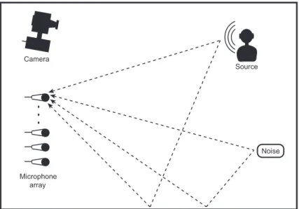
The localization of sources of emitting signals has been the focus of attention for more than a cen-tury. Localization and aiming in addition to noise and interference rejection allow microphone arrays to outperform single microphone systems. Arrays of microphones have a variety of ap-plications in speech data acquisition systems. Apap-plications include teleconferencing, biomedical devices for hearing impaired persons, audio surveillance, gunshot detection and camera pointing systems. The fundamental requirement for sensor array systems is the ability to locate and track a signal source. In addition to having high accuracy, the location estimator must be capable of a high update rate at reasonable computational cost in order to be useful for real time tracking and beamforming applications. Source location data may also be used for purposes other than beamforming, such as aiming a camera in a video conferencing system (Fig.1.1).

Microphone array

Camera

Noise Source

Figure 1.1: Sound source localization problem in an enclosed area.

Many current SSL systems assume that the sound sources are distributed on a horizontal plane [2]. This assumption simplifies the problem of SSL in almost all methods. In teleconference

(6)

CHAPTER 1. INTRODUCTION 2 plications they assume all talkers speak at the same height which is somewhat true, but the talker or other attendees can act as sound blockades between the main talker and the array, which is typically a linear wall-mounted microphone array. Moreover, in most dominant SSL methods, the computational cost for two dimensional cases is high so that the real time implementation needs a computer with high processing power. Some of these SSL methods have been modified to cover a three dimensional space at a very high computational cost. There is thus a need for a SSL tech-nique in 3D space that can be implemented in real time without requiring high computational power. There is also another problem to take into account, that is the reflections of the sound sig-nal in the different walls, floor or objects which there are around. These reflections interfere in the system making more difficult the localization so then, the SSL systems must be robust and work in adverse conditions: noisy and reverberant environments (see Fig.1.1).

Figure 1.2: Videoconferencing room (Cisco Telepresence 3000).

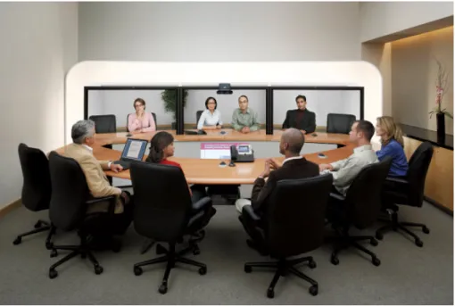
In this work we propose to use an improved SSL technique to develop an automatic voice-steering camera application. The objective is to be able to localize the members of a videoconferece taking place in a room. To this aim the implemented algorithm must be able to work in real time so its computational cost can not be as high as the conventional SSL algorithms. Moreover, taking into account that the speakers are quite close each one to the others, the technique employed must be robust and precise enough to identify correctly the main speaker. Once the speaker is located, the coordinates of his/her position are sent to a camera which points to the face of the member who is talking in this moment, making the video conference more similar to face to face communication (see Fig.1.2).

This Master’s thesis is organized as follows. In Chapter 2, conventional SSL techniques are re-viewed. Chapter 3 discusses the advantages of a modified SSL algorithm proposed by the author.

(7)

CHAPTER 1. INTRODUCTION 3 This approach is compared to other SSL methods in Chapter 4. Chapter 5 introduce a speaker detection based on the statistics of the resulting location estimates by the proposed SSL algorithm. The application of this approach and the speaker detector to videoconferencing environment is shown in Chapter 6. Finally, the conclusions obtained from all these experiments are presented in Chapter 7.

(8)

Chapter 2 Sound Source Localization

Sound Source Localization (SSL) is the process of determining the spatial location of a sound source based on multiple observations of the emitted sound signal [15]. The existing strategies of SSL may broadly be divided into two main classes: indirect and direct approaches [14]. Indi-rect approaches to source localization are usually two-step methods: first, the relative time delays for the various microphone pairs are evaluated and then the source location is found as the in-tersection of a pair of a set of half-hyperboloids centered around the different microphone pairs. Each half-hyperboloid determines the possible location of a sound source based on the measure of the time difference of arrival between the two microphones. On the other hand, direct approaches generally scan a set of candidate source positions and pick the most likely candidate as an estimate of the sound source location, thus performing the localization in a single step.

For both approaches, techniques such as the Generalized Cross-Correlation (GCC) method, proposed by Knapp and Carter in 1976, are widely used [13]. The Time Delay Estimation (TDE) be-tween signals from any pair of microphones can be performed by computing the cross-correlation function of the two signals after applying a suitable weighting step. The lag at which the cross-correlation function has its maximum is taken as the time delay between them.

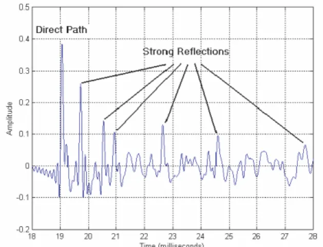
The type of weighting used with GCC is crucial to localization performance. Among several types of weighting, the phase transform (PHAT) is the most commonly used pre-filter for the GCC because it is more robust against reverberation. The GCC with the phase transform (GCC-PHAT) approach has been shown to perform well in a mild reverberant environment. Unfortunately, in the presence of even moderate reverberation levels, the algorithm is seriously hampered, due to the presence of spurious peaks. Also reflections of the signal on the walls make appear different peaks in the impulse response of the room which can generate peaks in the GCC function that may be strongest than the peak corresponding to the direct path. An example room impulse response is shown Figure 2.1.

Another class of important SSL algorithms is that based on a steered beamformer. When the source location is not known, a beamformer can be used to scan over a predefined spatial region by adjusting its steering parameters. The output of a beamformer is known as the steered response. When the point or direction of scan matches the source location, the SRP will be maximized.

(9)

CHAPTER 2. SOUND SOURCE LOCALIZATION 5

Figure 2.1: Room impulse response from source to one microphone.

ever, the localization performance of the conventional steered-beamformer techniques which ap-ply filters to the array signals have been derived to improve its performance. When the phase transform filter is incorporated with the steered-beamformer method, the resulting algorithm (SRP-PHAT) is superior in combating the adverse effects of background noise and reverberation compared to the conventional steered-beamformer method and the pairwise method, GCC-PHAT [13].

In the present day, the SRP-PHAT algorithm has become the most popular localization method for its good robust performance in real environment. However, the computational requirements of the method are large and this makes real-time implementation difficult. Since the SRP-PHAT method was proposed, there have been several attempts to reduce the computational require-ments of the intrinsic SRP search process [16],[4].

Other approaches to sound localization include Multiple Signal Classification (MUSIC) [11], [23], and Maximum Likelihood (ML) estimation [24], though these are typically applied to far-field narrow band direction-of- arrival estimation problems [15].

In the next subsections we introduce the concept of time delay estimation which is necessary for the SSL task. Then, the SRP is deeply explained when using the phase transform pre-filter.

2.1 Time Difference Of Arrival (TDOA)

Most practical acoustic source localization schemes are based onTime Delay Of Arrivalestimation (TDOA) for the following reason: such systems are conceptually simple. They are reasonably effective in moderately reverberant environments and, moreover, their low computational com-plexity makes them well-suited to real-time implementation with several sensors [21].

In general, an array is composed ofM microphones, and each microphone is positioned at a unique spatial location. Hence, the direct-path sound waves propagate along M bearing lines,

(10)

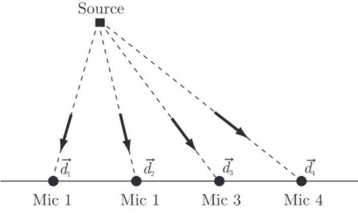
CHAPTER 2. SOUND SOURCE LOCALIZATION 6 from the source to each microphone, simultaneously. The orientations of these lines in the global coordinate system define the propagation directions of the wave fronts at each microphone. The propagation vectors for a four-element (m = 1, . . . ,4), linear array are illustrated in Figure 2.2, denoted asdm.~

Source

Mic 1 Mic 1 Mic 3 Mic 4

d2

d1 d3 d4

Figure 2.2: Propagation vectors.

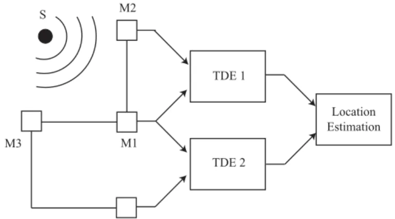
Time Delay Estimation (TDE) is concerned with the computation of the relative TDOA between different microphone sensors. It is a fundamental technique in microphone array signal processing and the first step in passive TDOA-based acoustic source localization systems. With this kind of localization, a two-step strategy is adopted as shown in Fig. 2.3.

The first stage involves estimation of the TDOA between receivers through the use of TDE techniques [5]. The estimated TDOAs are then transformed into range difference measurements between sensors, resulting in a set of nonlinear hyperbolic range difference equations. The sec-ond stage utilizes efficient algorithms to produce an unambiguous solution to these nonlinear hyperbolic equations. The solution produced by these algorithms result in the estimated position location of the source [19]. This data along with knowledge of the microphone positions are then used to generate hyperbolic curves, which are then intersected in some optimal sense to arrive at a source location estimate as shown in Figure 2.4.

Several variations of this principle have been developed [20]. They differ considerably in the method of derivation, the extent of their applicability (2D versus 3D, near field source versus far field source), and their means of solution.

2.2 SRP using the Phase Transform (PHAT)

Array signal processing techniques rely on the ability to focus on signals originating from a partic-ular location or direction in space. Most of these techniques employ some type of beamforming, which generally includes any algorithm that exploits an array’s sound-capture ability [12]. Beam-forming, in the conventional sense, can be defined by a filter-and-sum process, which applies some

(11)

CHAPTER 2. SOUND SOURCE LOCALIZATION 7 S M1 M2 M3 TDE 1 TDE 2 Location Estimation

Figure 2.3: A two stage algorithm for sound source localization.

Sensors Location Estimate 1 2 3 Hyperbola from (1,2) Hyperbola from (1,3) Hyperbola from (2,3)

Figure 2.4: Source estimation with three microphones.

temporal filters to the microphone signals before summing them to produce a single, focused sig-nal. These filters are often adapted during the beamforming process to enhance the desired source signal while attenuating others. The simplest filters execute time shifts that have been matched to the source signals propagation delays. This method is referred to as delay-and-sum beamforming; it delays the microphone signals so that all versions of the source signal are time-aligned before they are summed. The filters of more sophisticated filter-and-sum techniques usually apply this time alignment as well as other signal-enhancing processes.

Beamforming techniques have been applied to both source-signal capture and source local-ization. If the location of the source is known (and perhaps something about the nature of the source signal is known as well), then a beamformer can be focused on the source, and its output becomes an enhanced version (in some sense) of the inputs from the microphones. If the location of the source is not known, then a beamformer can be used to scan, or steer, over a predefined spatial region by adjusting its steering delays (and possibly its filters). As previously commented, the output of a beamformer, when used in this way, is known as the steered response. The SRP may peak under a variety of circumstances, but with favorable conditions, it is maximized when

(12)

CHAPTER 2. SOUND SOURCE LOCALIZATION 8 the steering delays match the propagation delays. By predicting the properties of the propagating waves, these steering delays can be mapped to a location, which should coincide with the location of the source.

For voice capture application, the filters applied by the filter-and-sum technique must not only suppress the background noise and contributions from unwanted sources, they must also do this in way that does not significantly distort the desired signal. The most common of these filters is the phase transform (PHAT), which applies a magnitude-normalizing weighting function to the cross-spectrum of two microphone signals.

We now describe the measurement principle of SRP-PHAT algorithm which is closely related to GCC-PHAT, and then introduce its implementation.

2.2.1 SRP-PHAT algorithm

Consider the output from microphonel,ml(t), in anM microphone system. Then, the SRP at the spatial pointx = [x, y, z]for a time framenof lengthT is defined as

Pn(x)≡ Z (n+1)T nT M X l=1 wlml(t−τ(x, l)) 2 dt, (2.1)

wherewlis a weight andτ(x, l)is the direct time of travel from locationxto microphonel. DiBiase [7] showed that the SRP can be computed by summing the GCCs for all possible pairs of the set of microphones. The GCC for a microphone pair(k, l)is computed as

Rmkml(τ) =

Z ∞

−∞

Φkl(ω)Mk(ω)Ml∗(ω)ejωτdω, (2.2) where τ is the time lag, ∗ denotes complex conjugation, Ml(ω) is the Fourier transform of the microphone signalml(t), andΦkl(ω) = Wk(ω)Wl∗(ω)is a combined weighting function in the frequency domain. The Phase Transform (PHAT) [13] has been demonstrated to be a very effective GCC weighting for time delay estimation in reverberant environments:

Φkl(ω)≡

1 |Mk(ω)M_l∗(ω)|

. (2.3)

Taking into account the symmetries involved in the computation of Eq.(2.1) and removing some fixed energy terms [7], the part ofPn(x)that changes withxis isolated as

P_n0(x) = M X k=1 M X l=k+1 Rmkml(τkl(x)), (2.4)

whereτkl(x)is theInter-Microphone Time-Delay Function(IMTDF). This function is very impor-tant, since it represents the theoretical direct path delay for the microphone pair (k, l) resulting from a point source located atx. The IMTDF is mathematically expressed as

(13)

τkl(x) =

kx−xkk − kx−xlk

c , (2.5)

wherecis the speed of sound, andxkandxlare the microphone locations.

The SRP-PHAT algorithm consists in evaluating the functionalP_n0(x)on a fine gridGwith the aim of finding the point-source locationxsthat provides the maximum value:

xs= arg max

x∈GP

0

n(x). (2.6)

2.2.2 Implementation

Basically, the SRP-PHAT algorithm is implemented as follows:

• Define a spatial gridGwith a given spatial resolutionr. The theoretical delays from each point of the grid to each microphone pair are pre-computed using Eq.(2.5).

• For each analysis frame, the GCC of each microphone pair is computed as expressed in Eq.(2.2).

• For each position of the gridx ∈ G, the contribution of the different cross-correlations are accumulated (using delays pre-computed in 1), as in Eq.(2.4).

• Finally, the position with the maximum score is selected. 2.2.3 Other modifications

The accuracy of the SRP-PHAT algorithm is limited by the time resolution of the PHAT weighted cross correlation functions [22]. However, despite its robustness, computational cost is a real issue because the SRP space to be searched has many local extrema [1]. Very interesting modifications have already been proposed to improve the SRP-PHAT algorithm. Some of this modifications only affect to the weighting factor. In [17] until five different weighting factors are proposed to improve the precision of the localization. Also exists the PHAT-β transform which varies the degree of spectral magnitude information (partial whitening) of each microphone signal using a single parameter, β, which varies from 0 (no whitening) to 1 (total whitening). A simulation study described in [10] considered the detection performance of sound sources using the PHAT-β and they have demonstrated that the standard PHAT (β= 1) improves detection performance for broadband signals. However, the optimal choice ofβtypically ranged between 0.5 and 0.8, which resulted in a significant performance improvements over both total (β=1) and no whitening (β=0).

Φkl(ω)≡

1

|M_k(ω)M_l∗(ω)|β. (2.7)

While many transforms consider improving SNR, the PHAT-βprimarily deconvolves the spec-trum so that each frequency region contributes more uniformly to the coherent sum of the steered power.

(14)

Figure 2.5: 2D example of SRC:jis the iteration index. The rectangular regions show the contract-ing search regions.

Other modifications of the SRP-PHAT algorithm are focused on reducing the computational cost of that technique. Examples of them are those based on Stochastic Region Contraction (SRC) [7] and Coarse-to-Fine Region Contraction (CFRC) [9]. The first proposes, using SRC, to make computing the SRP practical. So it is given an initial rectangular search volume containing the desired global optimum and perhaps many local maxima or minima, gradually, in an iterative process, contract the original volume until a sufficiently small subvolume is reached in which the global optimum is trapped (see Fig. 2.5). The second proposal uses a CFRC to make computing the SRP practical as well. Using CFRC can reduce the computational cost by more than three orders of magnitude [8].

(15)

Chapter 3 Improved SRP-PHAT algorithm for

Source Localization

A different strategy for implementing a less cost computational SRP-PHAT algorithm is shown in this section. The algorithm proposed instead of evaluating the SRP functional at discrete positions of a spatial grid, it is integrated over the GCC lag space corresponding to the volume surrounding each point of the grid [6].

3.1 The Inter-Microphone Time Delay Function

As commented in the previous chapter, the IMTDF plays a very important role in the source lo-calization task. This function can be interpreted as the spatial distribution of possible TDOAs resulting from a given microphone pair geometry.

-5 _-3 -1 ₁ 3 _{5 -5} -3 -1 1 3 -15 -10 -5 0 5 10 15 x Time delay - (ms) Three-dimensional representation of (m) τkl(x,y) 5 y(m)

Figure 3.1: Example of IMTDF. Representation for the planez = 0with microphones located at [−2,0,0]and[2,0,0].

(16)

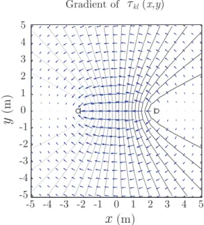
CHAPTER 3. IMPROVED SRP-PHAT ALGORITHM FOR SOURCE LOCALIZATION 12 The functionτkl(x)is continuous inxand changes rapidly at points close to the line connect-ing both microphone locations. Therefore, a pair of microphones used as a time-delay sensor is maximally sensible to changes produced over this line. An example function is depicted in Figure 3.1 for the planez= 0, withxk= [−2,0,0]andxl= [2,0,0]. The gradient of the function is shown in Figure 3.2. -5 -4 -3 -2 -1 0 1 2 3 4 5 -5 -4 -3 -2 -1 0 1 2 3 4 5

x

(m)

y

(m) Gradient of τkl (x,y)

Figure 3.2: Example of IMTDF. Gradient.

It is useful here to remark that the equation|τkl(x)|=C, withCbeing a positive real constant, defines a hyperboloid in space with foci on the microphone locationsxk andxl. Moreover, the set of continuous confocal half-hyperboloidsτkl(x) = C withC ∈ [−Cmax, Cmax], beingCmax = (1/c)kxk−xlk, spans the whole three-dimensional space.

At this point we can formulate the next theorem: Given a volumeV in space, the IMTDF for

points insideV,τkl(x∈V), takes only values in the continuous range[min (τkl(x∈∂V)),max (τkl(x∈∂V))], where∂V is the boundary surface that enclosesV.

In order to prove the theorem above, let us assume that a point inside V, x0 ∈ V, takes the maximum value in the volume, i.e. τkl(x0) = max (τkl(x∈V)) = CmaxV. Since there is a

half-hyperboloid that goes through each point of the space, all the points besidesx0satisfyingτkl(x) = CmaxV will also take the maximum value. Therefore, all the points on the surface resulting from

the intersection of the volume and the half-hyperboloid will take this maximum value, including those pertaining to the boundary surface ∂V. The existence of the minimum in∂V is similarly deduced.

The above property is very useful to understand the advantages of the approach presented in this work. Note that the SRP-PHAT algorithm is based on accumulating the values of the different GCCs at those time lags coinciding with the theoretical inter-microphone time delays, which are

(17)

CHAPTER 3. IMPROVED SRP-PHAT ALGORITHM FOR SOURCE LOCALIZATION 13 only computed at discrete points of a spatial grid. However, as described before, it is possible to analyze a complete spatial volume by scanning the time-delays contained in a range defined by the maximum and minimum values on its boundary surface. In the section 3.2, we describe how this knowledge can be included in the localization algorithm to increase its robustness.

-5 -4 -3 -2 -1 0 1 2 3 4 5 -5 -4 -3 -2 -1 0 1 2 3 4

5Intersecting Half-Hyperboloids for a Point-Source

x (m) x (m) -5 -4 -3 -2 -1 0 1 2 3 4 5 -5 -4 -3 -2 -1 0 1 2 3 4

5 Intersecting Half-Hyperboloids for a Point-Source

(a) (b)

y

(m)

y

(m)

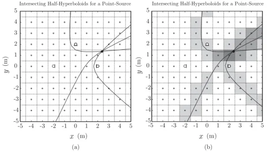
Figure 3.3: Intersecting half-hyperboloids and localization approaches. (a) Conventional SRP-PHAT. (b) Proposed.

3.2 Proposed Approach

Let us begin the description of the proposed approach by analyzing a simple case where we want to estimate the location xs of a sound source inside an anechoic space. In this simple case, the GCCs corresponding to each microphone pair are delta functions centered at the corresponding inter-microphone time-delays: Rmkml(τ) = δ(τ −τkl(xs)). For example and without loss of

gen-erality, let us assume a set-up withM = 3 microphones, as depicted in Figure 3.3(a). Then, the source position would be that of the intersection of the three half-hyperboloidsτkl(x) = τkl(xs), with (k, l) ∈ {(1,2),(1,3),(2,3)}. Consider now that, to localize the source, a spatial grid with resolution r = 1 m is used as shown in Figure 3.3(a). Unfortunately, the intersection does not coincide with any of the sampled positions, leading to an error in the localization task. Obviously, this problem would have been easier to solve with a two step localization approach, but the above example shows the limitations imposed by the selected spatial sampling in SRP-PHAT, even in optimal acoustic conditions. This is not the case of the approach followed to localize the source in Figure 3.3(b) where, using the same spatial grid, the GCCs have been integrated for each sam-pled position in a range that covers their volume of influence. A darker gray color indicates a greater accumulated value and, therefore, the darkest area is being correctly identified as the one containing the true sound source location. This new modified functional is expressed as follows

(18)

CHAPTER 3. IMPROVED SRP-PHAT ALGORITHM FOR SOURCE LOCALIZATION 14 P_n00(x) = M X k=1 M X l=k+1 Lkl2(x) X τ=Lkl1(x) Rmkml(τ). (3.1)

The problem is to determine correctly the limits Lkl1(x) and Lkl2(x), which depend on the specific IMTDF resulting from each microphone pair. The computation of these limits is explained in the next subsection.

3.2.1 Computation of integration limits

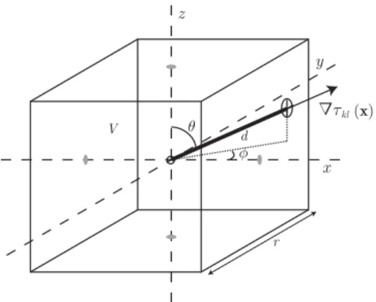
θ φ Δ τkl(x) d V x y z r

Figure 3.4: Volume of influence of a point in a rectangular grid.

As explained in Section 3.1, the IMTDF inside a volume can only take values in the range defined by its boundary surface. Therefore, for each point of the grid, the problem of finding the GCC integration limits of its volume of influence can be simplified to finding the maximum and minimum values on the boundary. To this end, it becomes useful to study the direction of the greatest rate of increase at each grid point, which is given by the gradient

∇τkl(x) = [∇xτkl(x),∇yτkl(x),∇zτkl(x)], (3.2) where ∇_xτkl(x) = ∂τkl(x) ∂x = 1 c _x₋_x k kx−xkk − x−xl kx−xlk , ∇yτkl(x) = ∂τkl(x) ∂y = 1 c _y₋_y k kx−xkk − y−yl kx−xlk , ∇zτkl(x) = ∂τkl(x) ∂z = 1 c _z₋_z k kx−xkk − z−zl kx−xlk . (3.3) The integration limits can be calculated for a symmetric volume by taking the product of the magnitude of the gradient and the distancedthat exists from the grid point to the intersection of

(19)

CHAPTER 3. IMPROVED SRP-PHAT ALGORITHM FOR SOURCE LOCALIZATION 15 a line with the gradient’s direction and the boundary:

Lkl1(x) =τkl(x)− k∇τkl(x)k ·d, (3.4) Lkl2(x) =τkl(x)) +k∇τkl(x)k ·d, (3.5) Figure 3.4 depicts the geometry for a rectangular grid with spatial resolutionr. For this cubic geometry, the distancedcan be expressed as

3.2.2 Computational Cost

LetLbe the DFT length of a frame andQ= M(M −1)/2the number of microphone pairs. The computational cost of SRP-PHAT is given by [18]:

SRP-PHATcost ≈[6.125Q2+ 3.75Q]Llog₂L

+15LQ(1.5Q−1) + (45Q2−30Q)ν0, (3.9) whereν0 is the average number of functional evaluations required to find the maximum of the SRP space. Since the cost added by the modified functional is negligible and the frequency-domain processing of our approach remains the same as the conventional SRP-PHAT algorithm, the above formula is valid for both approaches. Moreover, since the integration limits can be pre-computed before running the localization algorithm, the associated processing does not involve additional computation effort. However the advantage of the proposed method relies on the reduced number of required functional evaluations ν0 for detecting the true source location, which results in an improved computational efficiency.

(20)

Chapter 4 SSL Comparative

First of all it was necessary to demonstrate that the modified SRP-PHAT algorithm proposed has a similar behavior to traditional SRP-PHAT, so different experiments have been carried out.

4.1 Description of the application

Different experiments with real and synthetic recordings were conducted to compare the perfor-mances of the conventional SRP-PHAT algorithm, the SRC algorithm (explained in 2.2.3) and our proposed method. First, theRoomsimMatlab package [3] was used to simulate an array of 6 mi-crophones placed on the walls of a shoe-box-shaped room with dimensions 4 m×6 m×2 m (Fig. 4.1). 6 m 4 m Height = 2 m Figure 4.1: Set-up.

4.2 Results

The simulations were repeated with two different reverberation times (T60= 0.2s and T60= 0.7s), considering 30 random source locations and different Signal-to-Noise Ratio (SNR) conditions. The resultant recordings were processed with 3 different spatial grid resolutions in the case of SRP-PHAT and the proposed method (r1 = 0.01m,r2= 0.1m andr3= 0.5m). Note that the number of

(21)

CHAPTER 4. SSL COMPARATIVE 17 functional evaluationsν0depends on the selected value ofr, havingν₁0 = 480×105,ν₂0 = 480×102 andν₃0 = 384. The implementation of SRC was the one made available by Brown University’s LEMS athttp://www.lems.brown.edu/array/download.html, using 3000 initial random points. The processing was carried out using a sampling rate of 44.1 kHz, with time windows of 4096 samples of length and 50% overlap. The simulated sources were male and female speech signals of length 5 s with no pauses. The averaged results in terms ofRoot Mean Squared Error (RMSE) are shown in Figure 4.2(a-c).

10 5 0 SNR (dB) RMSE 2.5 2 1.5 1 0.5 0 r = 0.01 m RMSE with grid resolution

SRC SRP-PHAT Proposed (a) 10 5 0 SNR (dB) RMSE 2.5 2 1.5 1 0.5 0 r = 0.1 m RMSE with grid resolution

SRC SRP-PHAT Proposed (b) T60 = 0.2 s T₆₀ = 0.7 s T60 = 0.2 s T60 = 0.7 s r = 0.5 m RMSE with grid resolution

SRC SRP-PHAT Proposed 10 5 0 SNR (dB) RMSE 2.5 2 1.5 1 0.5 0 (c) T₆₀ = 0.2 s T60 = 0.7 s

Figure 4.2: Results with simulations. (a)r= 0.01m. (b)r= 0.1m. (c)r= 0.5m.

Since SRC does not depend on the grid size, the SRC curves are the same in all these graphs. As expected, all the tested systems perform considerably better in the case of low reverberation and high SNR. For the finest grid, it can be clearly observed that the performance of SRP-PHAT and the proposed method is almost the same. However, for coarser grids, our proposed method is only slightly degraded, while the performance of SRP-PHAT becomes substantially worse, specially for low SNRs and high reverberation. SRC has similar performance to SRP-PHAT withr = 0.01 m. Therefore, our proposed approach performs robustly with higher grid sizes, which results in a great computational saving in terms of functional evaluations, as depicted in Figure 4.3.

(22)

CHAPTER 4. SSL COMPARATIVE 18 (e) 2 3 4 5 6 7 8 r = 0.01 m _r = 0.1 m r = 0.5 m log10( ν) Functional Evaluations SRC SRP-PHAT Proposed

Figure 4.3: Functional evaluations.

r 0.01 0.1 0.5

ν0 802·105 802·102 641

SRP-PHAT RMSE = 0.29 RMSE = 0.74 RMSE = 1.82 Proposed RMSE = 0.21 RMSE = 0.29 RMSE = 0.31

SRC RMSE = 0.34 (ν0 = 58307)

Table 4.1: RMSE for the real-data experiment.

On the other hand, a real set-up quite similar to the simulated one was considered to study the performance of the method in a real scenario. Six omnidirectional microphones were placed at the 4 corners and at the middle of the longest walls of a videoconferencing room with dimensions 5.7 m×6.7 m×2.1 m and 12 seats. The measured reverberation time wasT60= 0.28s. The processing was the same as with the synthetic recordings, using continuous speech fragments obtained from the 12 seat locations. The results are shown in Table 4.1 and confirm that our proposed method performs robustly using a very coarse grid.

Although similar accuracy to SRC is obtained, the number of functional evaluations is signifi-cantly reduced.

Figure 4.4 shows that, for a fine grid, there is no difference between traditional and modified SRP-PHAT method. Note that the GCC resulting from each pair of microphones cross in the same point with equal accuracy. However, figures (a) and (b) of Fig.4.5 show that the results of localization when a coarse grid is used in the GCC calculations have not equal accuracy if traditional or modified SRP-PHAT is applied. It can be seen that when a coarse grid is used in order to get lower computational cost, the traditional SRP-PHAT approach has not enough accuracy to find the SSL while the proposed modified SRP-PHAT is precise enough.

(23)

CHAPTER 4. SSL COMPARATIVE 19

Figure 4.4: Source likelihood map. Fine grid (a) traditional and (b) modified SRP-PHAT.

Another way to evaluate the benefits of our proposed approach is by looking at the results shown in Table 4.2. It shows the percentage of correct frames were the source was correctly located using our proposed approach and the conventional SRP-PHAT algorithm. A frame estimate is considered to be erroneous if its deviation from the true source location is higher than 0.4 m, which is approximately the maximum deviation admissible for the coarser grid. Notice that, for the worst case (T60= 0.7and SNR= 0dB), the proposed approach is capable of localizing correctly the source with 74% correctness withr = 0.5m, which is approximately the performance achieved by the conventional algorithm usingr = 0.01m. Thus, our proposed approach provides similar performance with a reduction of five orders of magnitude in the required number of functional

Method (T60) Source 1 Source 2 Source 3

SNR= 10dB SNR= 5dB SNR= 0dB r(m) 0.01 0.1 0.5 0.01 0.1 0.5 0.01 0.1 0.5 SRP (0.2 s) 100 90 76 99 89 63 89 71 35 Prop. (0.2 s) 100 100 100 100 99 99 90 89 87 SRP (0.7 s) 100 89 64 96 81 52 75 66 21 Prop. (0.7 s) 100 100 99 98 98 98 78 74 74

(24)

CHAPTER 4. SSL COMPARATIVE 20

(a)

(b)

Figure 4.5: Source likelihood map. Coarse grid (a) traditional and (b) modified SRP-PHAT.

evaluations. Notice also that both methods perform almost the same in all situations when the finest grid is used.

(25)

Chapter 5 Speaker detection

A method for speaker detection based on the statistics of the resulting location estimates is pro-vided in this section. The proposed speaker detection method is based on the probability density function of the location estimates by the improved SRP-PHAT algorithm explained in Chapter 3.

5.1 Speaker Detection

In the next subsections, we describe how active speakers are detected in our system, which re-quires a previous discrimination between speech and non-speech frames based on the distribu-tion of locadistribu-tion estimates. To this end, we model the probability density funcdistribu-tion of the obtained locations when there are active speakers and when silence and/or noise is present.

5.1.1 Distribution of Location Estimates

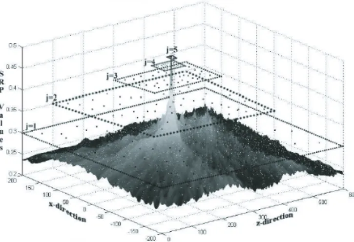
Our first step to speaker detection is to analyze the distribution of the location estimatesxˆswhen there is an active speaker talking inside the room from a static position. In this context, six mi-crophones were placed on the walls of the videoconferencing room and a set of 12 recordings from different speaker positions were analyzed to obtain the resulting location estimates. Fig-ure 5.1 shows an example of three two-dimensional histograms obtained from different speaker locations. It can be observed that, since the localization algorithm is very robust, the resulting distributions when speakers are active are significantly peaky. Also, notice that the shape of the distribution is very similar in all cases but centered in the actual speaker location. As a result, we model the distribution of estimates as a bivariate Laplacian as follows:

p(ˆxs|Hs(xs)) = 1 2σxσy exp− √ 2 _| x−xs| σx + |y−ys| σy , (5.1)

where p(ˆxs|Hs(xs))is the conditional probability density function (pdf) of the location esti-mates under the hypothesis Hs(xs)that there is an active speaker located atxs = [xs, ys]. Note that the variancesσ2_xandσ_y2may depend on the specific microphone set-up and the selected pro-cessing parameters. This dependence will be addressed in future works.

(26)

CHAPTER 5. SPEAKER DETECTION 22 0 10 20 30 40 x y x y x y x -3 -1 1 -3.5 -1.75 1.75 0 10 20 30 40 y y _x 0 10 20 30 40 x 3 3.5 0 -3 -1 1 -3.5 -1.75 1.75 y 3 3.5 0 -3 -1 1 -3.5 -1.75 1.75 3 3.5 0

Figure 5.1: Distribution obtained for three different speaker locations.

On the other hand, a similar analysis was performed to study how the distribution changes when there are not active speakers, i.e. only noise frames are being processed. The resulting histogram can be observed in Figure 5.2, where it becomes apparent that the peakedness of this distribution is not as significant as the one obtained when there is an active source. Taking this into account, the distribution of non-speech frames is modeled as a bivariate Gaussian:

p(ˆxs|Hn) = 1 2πσxnσyn exp− x2 2σ_xn2 + y2 2σ_yn2 , (5.2)

wherep(xˆs|Hn)is the conditional pdf of the location estimates under the hypothesisHnthat there are not active speakers, and the variancesσ2_x_nandσ_y2_nare those obtained with noise-only frames.

0 10 20 30 40 50 60 x -3 -1 1 -3.5 -1.75 1.75 y 3 3.5 0

Figure 5.2: Distribution for non-speech frames.

5.1.2 Speech/Non-Speech Discrimination

In the above subsection, it has been shown that speech frames are characterized by a bivariate Laplacian probability density function. A similar analysis of location estimates when there are not active speakers results in a more Gaussian-like distribution, which is characterized by a shape less

(27)

CHAPTER 5. SPEAKER DETECTION 23 peaky than a Laplacian distribution. This property is used in our system to discriminate between speech and non-speech frames by observing the peakedness of a set of accumulated estimates:

C=       ˆ xs(n) yˆs(n) ˆ xs(n−1) ysˆ (n−1) .. . ... ˆ xs(n−L−1) ysˆ(n−L−1)       = [cxcy], (5.3)

whereLis the number of the accumulated estimates in matrixC. A peakedness criterion based on high-order statistics was evaluated. In probability theory and statistics, kurtosis is a measure of the ”peakedness” of the probability distribution of a real-valued random variable.

Figure 5.3: Excess Kurtosis for different density distributions.

Fig. 5.3 is an example where are compared several well-known distributions from different parametric families. All densities considered are unimodal and symmetric. Each has a mean and skewness of zero. Parameters were chosen to result in a variance of unity in each case. The seven densities are:

• D: Laplace distribution, red curve (two straight lines in the log-scale plot), excess kurtosis = 3

• S: hyperbolic secant distribution, orange curve, excess kurtosis = 2 • L: logistic distribution, green curve, excess kurtosis = 1.2

• N: normal distribution, black curve (inverted parabola in the log-scale plot), excess kurtosis = 0

• C: raised cosine distribution, cyan curve, excess kurtosis = -0.593762... • W: Wigner semicircle distribution, blue curve, excess kurtosis = -1

(28)

CHAPTER 5. SPEAKER DETECTION 24 • U: uniform distribution, magenta curve (shown for clarity as a rectangle in the image), excess

kurtosis = -1.2.

Kurtosis is defined as a normalized form of the fourth central momentµ4: Kurt(cx)≡

µ4 µ2 2

, (5.4)

where µi denotes theith central moment (and in particular, µ2 is the variance). The excess Kurtosis is defined by:

γ2 ≡ µ4 µ2 2

−3, (5.5)

Since the kurtosis of a normal distribution equals 3, we propose the following discrimination rules for active speech frames:

Kurt(cx) ( ≥3 speech <3 non−speech , (5.6) Kurt(cy) ( ≥3 speech <3 non−speech , (5.7)

where a frame is selected as speech if any of the above conditions is fulfilled. 5.1.3 Camera Steering

To provide a suitable camera stability, a set of target positions were pre-defined coinciding with the actual seats in the videoconferencing room. The localization system will be responsible for communicating the camera which of the target positions is currently active. This process involves two main steps. First, it is necessary to discriminate between speech and non-speech frames as explained in Section 5.1.2. If a burst of speech frames is detected, then the estimated target po-sition is forwarded to the camera when it does not match the current target seat. Since all the target positions are assumed to have the same prior probability, a maximum-likelihood criterion is followed:

ˆ

xt= arg max_x

t

p(ˆxs|H(xt)), t= 1. . . Nt, (5.8) where xt is one of theNt pre-defined target positions. Given that the likelihoods have the same distribution centered at different locations, the estimated target positionxˆtis the one which is closest to the estimated locationˆxs.

(29)

Chapter 6 Application to Videoconferencing

The SSL method explained in the chapter 3 has been applied in a videoconference system where, by accurately estimating the various users physical locations, it would be possible to steer a video camera toward the currently active speaker.

6.1 Set up for the videoconferece

To evaluate the performance of our proposed approach a set of recordings was carried out in a videoconferencing test room with dimensions 6.67 m x 5.76 m x 2.10 m. A set of 6 omnidirectional microphones were placed on the walls of the room.

To be precise, 4 of the microphones were situated at the 4 corners of the ceiling of the room and the other two microphones were placed at the same height but in the middle of the longest walls. Figure 6.1 shows the microphone set-up, the camera location and the different seats occupied by the participants. Black dots represent the 12 pre-defined target locations used to select the active speaker seat.

Camera Mic.1

Mic.2 Mic.3

Mic.4 Mic.5 Mic.6

6.67 m

5.76 m

Figure 6.1: Room for the videoconference.

(30)

CHAPTER 6. APPLICATION TO VIDEOCONFERENCING 26 Grid res. 0.5 m 0.3 m L 5 10 15 20 5 10 15 20 % SP 52.5 60.4 70.0 74.0 68.9 70.7 83.1 85.4 % N-SP 75.9 64.8 70.9 72.7 81.4 70.9 81.5 82.3 % T 98.2 99.6

Table 6.1: Performance in Terms of Percentage of Correct Frames

6.2 Description of the application

The experiment consisted in recording speakers talking from the different target positions (only one speaker at each time) with the corresponding space of silence between two talking interven-tions. The recordings were processed with the aim of evaluating the performance of our system in discriminating speech from non-speech frames and determining the active speaker so that the camera can point at the correct seat. With this aim, the original recordings were manually labeled as speech and non-speech fragments. The processing used a sampling rate of 44.1 kHz, with time windows of 2048 samples and 50% overlap. The location estimates were calculated using the modified SRP-PHAT functional, as explained in Chapter 3.

The discrimination between speech and non-speech frames was carried out by calculating the kurtosis of the last L estimated positions, as explained in Chapter 5.

6.3 Results

Modified SRP-PHAT approach joint the speech/non-speech discriminator have been used for a videoconference application, so different experiments have been carried out.

A new experiment was carried out in order to check the behavior of the speech/non-speech discriminator. To this aim, a set of recordings made in the test room (see Fig. 6.1) were used. These recordings were made from different pre-defined locations and they consist in active and non-active speakers, which is the same as people talking and noise environment.

Table 6.3 shows the percentage of correctly detected speech (% SP) and non-speech (% N-SP) frames with different number of accumulated positionsL= 5,10,15,20. Moreover, the processing was performed considering two different spatial grid sizes (0.3 m and 0.5 m). The percentage of speech frames with correct target positions (% T) is also shown in the table. It can be observed that, generally, the performance increases with a finer grid and with the number of accumulated estimatesL. These results were expectable, since the involved statistics are better estimated with a higher number of location samples. Although it may seem that there are a significant number of speech frames that are not correctly discriminated, it should be noticed that this is not a prob-lem for the correct driving of the camera, since most of them are isolated frames inside speech fragments that do not make the camera change its pointing target.

(31)

Chapter 7 Summary and Conclusions

Sound source localization and speech/non-speech detection techniques have been presented in this work to be used in a multiparticipant videoconferencing environment with a microphone array system for a steering-camera application.

Based on the well known SRP-PHAT SSL method, a modified version of that technique that uses a new functional has been developed. The proposed functional is based on the accumu-lation of GCC values in a range that covers the volume surrounding each point of the defined spatial grid. The GCC integration limits are determined by the gradient of the inter-microphone time delay function corresponding to each microphone pair, thus, taking into account the spatial distribution of possible TDOAs resulting from a given array geometry. Our results showed that the proposed approach provides similar performance to the conventional SRP-PHAT algorithm in difficult environments with a reduction of five orders of magnitude in the required number of functional evaluations. This reduction has been shown to be sufficient for the development of real-time source localization applications.

In a videoconferencing environment where the sources are voices from different speakers, a speech/non-speech detection step is necessary to provide a robust steering camera system. For this reason the distribution of location estimates has been obtained using the proposed SRP-PHAT functional. Our analysis shows that location estimates follow different distributions when speak-ers are active or mute. This fact allows us to discriminate between speech and non-speech frames under a common localization framework. The results of experiments conducted in a real room suggest that, using a moderately high number of accumulated location estimates, it is possible to discriminate with significant accuracy between speech and non-speech frames, which is sufficient to correctly detect an active speaker and point the camera towards his/her predefined location.

To summarize, a modified SRP-PHAT algorithm for real-time SSL has been developed and evaluated in a practical scenario. The proposed method has been integrated into a speaker detec-tion step to localize active sources in a videoconferencing room. In this context, a videocamera can be successfully driven by using the locations provided by our combined approach, showing the capabilities of the contributions described in this Master’s thesis.

(32)

Chapter 8 Acknowledgments

This work was supported by the Ministry of Education and Science under the project TEC2009-14414-C03-01.

(33)

Bibliography

[1] AARABI, P. The fusion of distributed microphone arrays for sound localization. EURASIP

Journal on Applied Signal Processing 2003(2003), 338–347.

[2] ALGHASSI, H. Eye Array Sound Source Localization. PhD thesis, University of British Columbia, 2008.

[3] CAMPBELL, D. R. Roomsim: a MATLAB simulation shoebox room acoustics, 2007. http://media.paisley.ac.uk/ campbell/Roomsim.

[4] CHAZHANG, D., FLORENCIO,ANDZHENGYOU, Z. Why does PHAT work well in low noise, reverberant environments. ICASSP, pp. 2565–8.

[5] CHEN, J., BENESTY, J., AND HUANG, Y. Time delay estimation in room acoustic environ-ments: an overview. EURASIP Journal on Applied Signal Processing 2006(2006), 1–19.

[6] COBOS, M., MARTI, A.,ANDLOPEZ, J. J. A modified srp-phat functional for robust real-time

sound source localization with scalable spatial sampling. IEEE Signal Processing Letters 18, 1 (January 2011).

[7] DIBIASE, J. H. A high accuracy, low-latency technique for talker localization in reverberant environ-ments using microphone arrays. PhD thesis, Brown University, Providence, RI, May 2000. [8] DO, H.,ANDSILVERMAN, H. F. A fast microphone array SRP-PHAT source location

imple-mentation using coarse-to-fine region contraction (CFRC). InProceedings of the IEEE Workshop on Applications of Signal Processing to Audio and Acoustics (WASPAA 2007)(2007).

[9] DO, H., SILVERMAN, H. F.,ANDYU, Y. A real-time SRP-PHAT source location

implementa-tion using stochastic region contracimplementa-tion (SRC) on a large-aperture microphone array. InIEEE International Conference on Acoustics, Speech and Signal Processing (ICASSP 2007)(2007). [10] DONOHUE, K. D., HANNEMANN, J.,AND DIETZ, H. G. Performance for phase transform

for detecting sound sources in reverberant and noisy environments. Signal Processing 87, 7 (July 2007), 1677–1691.

[11] FRIEDLANDER, B.,ANDWEISS, A. J. Direction finding for wide-band signals using an

inter-polated array. IEEE Transactions on Signal Processing(April 1993), 41:1618:1634.

(34)

BIBLIOGRAPHY 30 [12] JOHNSON, D. H.,ANDDUDGEON, D. E.Array Signal Processing: Concepts and Techniques.P T

R Prentice Hall, 1993.

[13] KNAPP, C. H., AND CARTER, G. C. The generalized correlation method for estimation of

time delay. Transactions on Acoustics, Speech and Signal Processing ASSP-24(1976), 320–327. [14] MADHU, N.,ANDMARTIN, R.Advances in Digital Speech Transmission. Wiley, 2008, ch.

Acous-tic source localization with microphone arrays, pp. 135–166.

[15] MUNGAMURU, B. Enhanced Sound Localization. PhD thesis, University of Toronto, 2003. [16] MUNGAMURU, B., AND AARABI, P. Enhanced sound localization. IEEE Trans Syst, Man,

Cybernet Part B: Cybernet 2004;34(3):152640.

[17] PIRINEN, T. W. An experimental comparison of time delay weights for deirection of arrival estimation. 11th Int. Conference on Digital Audio Effects DAFx-08(2008), 1–4.

[18] SILVERMAN, H. F., YU, Y., SACHAR, J. M.,ANDPATTERSONIII, W. R. Performance of real-time source-location estimators for a large-aperture microphone array. IEEE Transactions on Speech and Audio Processing 13(2005), 593–606.

[19] STOICA, P.,ANDLI, J. Source localization from range-difference measurements. IEEE Signal

Processing Magazine(November 2006), 63–69.

[20] SVAIZER, P., MATASSONI, M., AND OMOLOGO, M. Acoustic source location in a three-dimensional space cross-power spectrum phase. Proc. IEEE Int. Conf. Acoust., Speech Signal Processing ICASSP-97(Munich, Germany, April 1997), 231–234.

[21] TELLAKULA, A. K. Acoustic source localization using time delay estimation. PhD thesis, Indiand Institute od Science, August 2007.

[22] TERVO, S.,ANDLOKKI, T. Interpolation methods for the srp-phat algorithm. The 11th

Inter-national Workshop on Acoustic Echo and Noise Control, Seattle, Washington, USA, IWAENC2008 (September 2008), 14–17.

[23] WANG, H., AND KAVEH, M. Coherent signal-subspace processing for the detection and estimation of angles of arrival of multiple wideband sources. IEEE Transactions on Acoustics, Speech, and Signal Processing(August 1985), ASSP–33:823:831.

[24] WATENABE, H., SUZUKI, M., NAGAI, N.,ANDMIKI, N. A method for maximum likelihood

bearing estimation without nonlinear maximization. Transactions of the Institute of Electronics, Information and Communication Engineers(August 1989), J72A, 8:303:308.

(35)

Audio Engineering Society

Convention Paper

Presented at the 128th Convention

2010 May 22–25 London, UK

The papers at this Convention have been selected on the basis of a submitted abstract and extended precis that have been peer reviewed by at least two qualified anonymous reviewers. This convention paper has been reproduced from the author’s advance manuscript, without editing, corrections, or consideration by the Review Board. The AES takes no responsibility for the contents. Additional papers may be obtained by sending request and remittance to Audio Engineering Society, 60 East 42nd Street, New York, New York 10165-2520, USA; also see www.aes.org. All rights reserved. Reproduction of this paper, or any portion thereof, is not permitted without direct permission from the Journal of the Audio Engineering Society.

On the Effects of Room Reverberation in 3D

DOA Estimation Using a Tetrahedral

Microphone Array

Maximo Cobos1_{, Jose J. Lopez}1_{and Amparo Marti}1

1

Institute of Telecommunications and Multimedia Applications (iTEAM), Universidad Polit´ecnica de Valencia, Valencia, Camino de Vera s/n, 46022, Spain

Correspondence should be addressed to Maximo Cobos ([email protected])

ABSTRACT

This paper studies the accuracy in the estimation of the Direction-Of-Arrival (DOA) of multiple sound sources using a small microphone array. As other sparsity-based algorithms, the proposed method is able to work in underdetermined scenarios, where the number of sound sources exceeds the number of microphones. Moreover, the tetrahedral shape of the array allows to estimate DOAs in the 3-dimensional space easily, which is an advantage over other existing approaches. However, since the proposed processing is based on an anechoic signal model, the estimated DOA vectors are severely affected by room reflections. Experiments to analyze the resultant DOA distribution under different room conditions and source arrangements are discussed using both simulations and real recordings.

1. INTRODUCTION

Source localization is still one of the most challeng-ing problems in acoustic signal processchalleng-ing. Estimat-ing thedirection of arrival (DOA) of multiple sound sources in a real scenario is a very difficult task. The estimation of DOAs of multiple sources has interest-ing applications in many speech processinterest-ing systems, such as hands-free devices, teleconference systems

or hearing aids. Algorithms for acoustic source lo-calization are often classified into direct approaches and indirect approaches [1]. Indirect approaches es-timate the time difference of arrival (TDOA) be-tween various microphone pairs and then, based on the array geometry, estimate the source positions by optimization techniques. On the other hand, direct approaches compute a cost function over a set of

(36)

Cobos et al. Effects of Reverberation in 3-D DOA Estimation

candidate locations and take the most likely source positions.

Cross-correlation-based methods, such as General-ized Cross Correlation (GCC) [2], are commonly applied in source localization. However, the GCC method becomes problematic when multiple sources are active simultaneously. Techniques based on the

Steered Response Power (SRP) are also popular in acoustic source localization, but computationally de-manding [3]. In the last years, localization meth-ods based on the estimation of TDOAs in the time-frequency domain have been receiving increasing at-tention [4][5]. These algorithms provide considerable good accuracy with reduced computational complex-ity using the phase differences observed from two closely spaced sensors. However, their performance is considerably worse in non-anechoic environments, since room reflections affect the variance of DOA estimates. Therefore, source localization remains a very challenging task.

Recently, the authors studied the effect of room reflections in source localization using a small mi-crophone array composed of three mimi-crophones [6], however, only the horizontal plane was considered. This paper discusses the accuracy achieved by a tetrahedral microphone array in 3-D source localiza-tion tasks. Following a sparsity-based approach, the microphone signals are transformed into the time-frequency domain. Then, phase-differences between microphone pairs are analyzed to provide an esti-mation of the DOA corresponding to the dominant source in each time-frequency bin. With the aim of discussing how the acoustic environment affects the distribution of DOA estimates in the 3-D space, a set of simulations considering different acoustic en-vironments has been carried out. The results show that the statistics of the DOA vector norm provide a good description of the environment where the sound sources were recorded.

The paper is structured as follows. Section 2 presents the assumed signal model and the proposed processing used to estimate the location of several sound sources. Section 3 shows how the distribution of DOA estimates changes depending on the acous-tic environment. Section 4 presents several experi-ments that analyze the statistical properties of DOA estimates using simulated rooms and real recordings.

Finally, the conclusions of this work are summarized in Section 5.

2. SIGNAL MODEL AND DOA ESTIMATION

2.1. Signal Model

The signals recorded by a microphone array, with sensors denoted with indicesm= 1,2, . . . , M in an acoustic environment where N sound sources are present, can be modeled as a finite impulse response convolutive mixture, written as

xm(t) = N X n=1 Lm−1 X `=0 hmn(`)sn(t−`), m= 1, . . . , M (1) wherexm(t) is the signal recorded at the m-th

mi-crophone at time samplet, sn(t) is the n-th source

signal,hmn(t) is the impulse response of the

acous-tic path from sourcen to sensor m, and Lm is the

maximum length of all impulse responses.

The above model can also be expressed in the short-time Fourier transform (STFT) domain as follows

Xm(k, r) =

N

X

n=1

Hmn(k)S(k, r), (2)

whereXm(k, r) denotes the STFT of them-th

mi-crophone signal, beingkand rthe frequency index and time frame index, respectively. Sn(k, r) denotes

the STFT of the source signalsn(t) and Hmn(k) is

the frequency response from sourcento sensor m.

2.1.1. Sparse Sources

In the time-frequency domain, source signals are usually assumed to be sparse. A sparse source has a peaky probability density function: the signal is close to zero at most time-frequency points, and has large values in rare occasions. This property has been widely applied in many works related to source signal localization [5][4] and separation [7][8] in un-derdetermined situations, i.e. when there are more sources than microphone signals.

If we assume that the sources rarely overlap at each time-frequency point, Equation (2) can be simplified as follows

Xm(k, r)≈Hma(k)Sa(k, r), (3)

AES 128th Convention, London, UK, 2010 May 22–25

(37)

Cobos et al. Effects of Reverberation in 3-D DOA Estimation

where Sa(k, r) is the dominant source at

time-frequency point (k, r). To simplify, we assume an anechoic model where the sources are sufficiently distant to consider plane wavefront incidence. Then, the frequency response is only a function of the time-delayτmnbetween each source and sensor

Hmn(k) =ej2πfkτmn, (4)

being fk the frequency corresponding to frequency

indexk. R 1 2 3 4 dn x z y p1 p2 p3 p4 θn φn

Fig. 1: Tetrahedral microphone array for 3-D DOA estimation.

2.2. Array Geometry and DOA Estimation

Now consider a tetrahedral microphone array (M = 4) with base radius R, as shown in Figure 1. The sensor location vectors in the 3-dimensional space with origin in the array base center, are given by:

p1 = [R, 0, 0] T , p2 = " −R 2, √ 3 2 R, 0 #T , p3 = " −R 2, − √ 3 2 R, 0 #T , p4 = h 0, 0, R√2i T . (5) (6) The DOA vector of then-th source as a function of the azimuthθn and elevationφnangles is defined as

dn= [cosθncosφn, sinθncosφn, sinφn] T

. (7)

The source to sensor time delay is given by τmn =

pT

mdn/c, beingcthe speed of sound. Therefore, the

frequency response of Equation (4) can be written as Hmn(k, r)≈ej 2πfk c p T mdn_. ₍₈₎

Taking into account this last result and Equation 3, it becomes clear that the phase difference between the microphone pair formed by sensors i and j, is given by 6 _X j(k, r) Xi(k, r) ≈ 2πfk c (pj−pi) T_d n, (9)

where6 _{denotes the phase of a complex number.}

Using a reference microphoneq, the phase difference information at point (k, r) ofM−1 microphone pairs is stored in the vector

bq(k, r) = 6 _X 1(k, r) Xq(k, r) , . . . ,6 _X M(k, r) Xq(k, r) T , (10) forming the following system of equations:

bq(k, r) = 2πfk c Pdn, (11) where P= [p1q, . . . ,pM q] T , pnq =pn−pq. (12)

Finally, the DOA at time-frequency bin (k, r) is ob-tained by taking the inverse of thePmatrix

ˆ

dn(k, r) =

c

2πfk

P−1bq(k, r). (13)

The regular tetrahedral geometry used in this paper leads to the following simple equations fordn(k, r) =

[ ˆd1, dˆ2, dˆ3]T: ˆ d1 = cosθncosφn= c 2πfk 1 √ 3(b2+b3), (14) ˆ d2 = sinθncosφn= c 2πfk (b3−b2), (15) ˆ d3 = sinφn= c 2πfk " 1 √ 6(b2+b3)− r 3 2b4 # , (16)

where bn is the n-th element of the vectorb1(k, r) (reference microphoneq = 1). The azimuth angle

(38)

Cobos et al. Effects of Reverberation in 3-D DOA Estimation 1 1 0.8 0.6 0.4 0.2 0 -0.2 -0.4 -0.6 -0.8 -1 1 0.8 0.6 0.4 0.2 0 -0.2 -0.4 -0.6 -0.8 -1 0.5 0 -0.5 -1 x y z (a) 3-D DOA Distribution 1 1 0.8 0.6 0.4 0.2 0 -0.2 -0.4 -0.6 -0.8 -1 1 0.8 0.6 0.4 0.2 0 -0.2 -0.4 -0.6 -0.8 -1 0.5 0 -0.5 -1 x y z (b) 3-D DOA Distribution 1 1 0.8 0.6 0.4 0.2 0 -0.2 -0.4 -0.6 -0.8 -1 1 0.8 0.6 0.4 0.2 0 -0.2 -0.4 -0.6 -0.8 -1 0.5 0 -0.5 -1 x y z (c) 3-D DOA Distribution

Fig. 2: Histograms showing the distribution of DOA estimates in the 3-D space calculated from a mixture of 4 speech sources. (a) Anechoic conditions. (b) T60= 150 ms. (c) T60= 300 ms.

is obtained using the four quadrant inverse tangent function:

ˆ

θn(k, r) = atan360

◦

( ˆd1,dˆ2). (17)

The elevation angle is directly obtained as ˆ

φn(k, r) = sin−1( ˆd3). (18)

Note that for each time-frequency point (k, r), es-timating the 3-D direction of arrival is relatively simple, just using the observed phase differences be-tween 3 microphone pairs of the array. Another as-pect to consider is spatial aliasing. The distance between microphones determines the angular alias-ing frequency. Due to the 2π ambiguity in the calculation of the phase differences, the maximum ambiguity-free frequency in a microphone pair sub-array would be given by fk =c/2d, where d is the

separation distance between the capsules. Beyond this frequency, there is no a one-to-one relationship between phase difference and spatial direction. How-ever, small arrays withd≈1.5 cm provide an unam-biguous bandwidth greater than 11 kHz, covering a perceptually important frequency range.

3. 3-D DOA DISTRIBUTIONS

The assumed signal model is close to reality when we are localizing in anechoic conditions. Obviously, the localization accuracy will be affected by room

reflections when the localization task is performed in a reverberant environment. Moreover, room re-flections also affect source sparseness [10] which is another basic assumption taken by the localization method.

In this section, we carry out some simulations con-sidering a rectangular room and using different wall conditions in order to show how the distribution of DOA estimates is affected by room reflections.

3.1. Deviation of DOA estimates

With the objective of showing how the proposed ar-ray is capable of capturing the 3-D spatial infor-mation of sound, we show a simulated sound scene where 4 speech sources are simultaneously active in a room (10 s duration). The azimuth angles of the sources were θ1 = 0◦, θ2 = 30◦, θ3 = 45◦ and

θ4 = 100◦. The elevation angles were φ1 = 0◦,

φ2 = 30◦, φ3 = −10◦ and φ4 = 45◦. With the aim of showing graphically how the distribution of DOA estimates changes depending on the degree of reverberation, the sound scene was simulated using an increasing wall reflection factor [9], thus allow-ing more reflections inside the room. A more de-tailed description of the simulation set-up is given in Section 4. Figure 2 shows the 3-D histograms that represent the amount of estimates produced in a given direction. Note how in the anechoic case (a), the sources appear as localized peaky zones corre-sponding to their real DOAs. The diffuseness added by room reflections can be clearly seen in (b)-(c),

(39)

Cobos et al. Effects of Reverberation in 3-D DOA Estimation 0 1 2 3 4 5 6 0 5 10 15 20 25 0 1 2 3 4 5 6 0 0.5 1 1.5 2 2.5 0 1 2 3 4 5 6 0 0.2 0.4 0.6 0.8 1 1.2 1.4 0 1 2 3 4 5 6 0 0.1 0.2 0.3 0.4 0.5 0.6 0.7 0.8 0.9 Anechoic T60 = 50 ms T60 = 150 ms T60 = 300 ms

Norm value Norm value Norm value Norm value

(a) (b) _(c) _(d)

Fig. 3: Distribution of the DOA vector norm for different room conditions. (a) Anechoic room. (b) T60= 50 ms. (c) T60= 150 ms. (d) T60= 300 ms.

where the estimates, although clustered around the real DOA directions, have been highly spread.

3.2. DOA vector norm distribution

It is important to note that perfectly estimated di-rections will have unit norm, i.e. ||ˆdn(k, r)|| = 1.

Therefore, perfect estimations fulfilling the used ane-choic model will lie on the unit sphere. In contrast, the norm of the estimated DOA vector in points with high spectral overlap between the sources or cor-rupted by reverberation will be further away from the unity. Figure 3 shows four examples of norm dis-tributions obtained from different simulated rooms with a single active source located atθ= 0◦_,_φ_{= 0}◦_.

Note that in the anechoic case, the resultant norm distribution has a very large peak in the unity, whereas in the case of reverberant rooms, the dis-tribution is substantially spread and asymmetric. In the next section, we will study in detail the effect that the source-to-array distance and the number of sources have in the DOA vector norm distribution for different room conditions.

4. EXPERIMENTS

As shown in the last section, the presence of room re-flections has a considerable effect on the estimated DOA vectors, since the anechoic signal model be-comes corrupted with reverberation. Thus, the di-rect path contribution is very important to obtain correct DOA estimates. Moreover, the sparseness assumption also becomes affected by reverberation and by the number of sources. In this section, we

conduct a set of experiments focused on the statisti-cal analysis of the resultant DOA norm distribution under different situations.

4.1. Simulations

Several sound scenes have been simulated to discuss some important aspects previously commented: re-verberation time, number of sources and direct-path contribution. In the simulations, a set of sound sources were positioned inside a shoe-box-shaped room (4 m × 3.6 m × 2.6 m) and all the source-to-sensor impulse responses were acquired by means of the mirror image method [9]. The wall reflection factor of the walls was changed to get different rever-beration times (anechoic, T60 = 50 ms, T60 = 150 ms and T60 = 300 ms). Different number of sound sources (speech) were considered:

• 1 source at (θ= 0◦, φ= 0◦). • 2 sources at 1. (θ1= 45◦,φ1= 0◦), 2. (θ2=−45◦,φ2= 0◦). • 4 sources at 1. (θ1= 0◦,φ1= 0◦), 2. (θ2= 90◦,φ2=−30◦), 3. (θ3= 180◦,φ3= 30◦), 4. (θ4=−90◦,φ4= 60◦).

Moreover, different distances from the sources to the array were taken into account to modify the