Efficient density-based methods for knowledge discovery in databases

knowledge discovery in databases

Von der Fakult¨at f¨ur Mathematik, Informatik und Naturwissenschaften der Rheinisch-Westf¨alischen Technischen Hochschule Aachen

zur Erlangung des akademischen Grades eines Doktors der Naturwissenschaften genehmigte Dissertation

vorgelegt von Diplom-Informatiker

Ralph Krieger aus K¨oln

Berichter: Universit¨atsprofessor Dr. rer. nat. Thomas Seidl Professor Dr. Bart Goethals

Tag der m¨undlichen Pr¨ufung: 09. Juli 2008

Diese Dissertation ist auf den Internetseiten der Hochschulbibliothek online verf¨ugbar

Acknowledgements 1

Abstract 2

Zusammenfassung 3

Density-based methods for knowledge discovery in

databases

5

I

Efficient density-based methods for clustering

13

1 Clustering multi-dimensional data 14

1.1 Full-space clustering . . . 14

1.2 Problems for clustering multi-dimensional data . . . 16

1.3 Solutions for clustering multi-dimensional data . . . 19

1.4 Basic notions . . . 24

2 Unbiased density-based subspace clustering 31 2.1 Introduction . . . 31

2.2 Related work . . . 32

2.3 Dimensionality bias . . . 34

2.4 An unbiased density estimator . . . 36

2.5 DUSC subspace clustering . . . 39

2.6 Apriori subspace clustering . . . 48

2.7 Experiments . . . 56

2.8 Conclusion . . . 61

3.1 Introduction . . . 63

3.2 Related work . . . 67

3.3 Density-based subspace clusters . . . 68

3.4 Depth-first multistep subspace clustering . . . 71

3.5 Indexing subspace clusters . . . 83

3.6 Experiments . . . 102

3.7 Conclusion . . . 114

4 Visualization of subspace clusters 115 4.1 Introduction . . . 116

4.2 Related work . . . 117

4.3 VISA . . . 118

4.4 Conclusion . . . 127

5 Efficient subspace clustering for multidimensional sequences 128 5.1 Introduction . . . 128

5.2 Related work . . . 131

5.3 Subspace subsequence cluster model . . . 131

5.4 Efficient subsequence cluster mining . . . 137

5.5 A subspace subsequence clustering algorithm . . . 143

5.6 Experimental evaluation . . . 149

5.7 Conclusion and further work . . . 158

II

Efficient density-based methods for

classifica-tion

159

6.2 Basic notations . . . 162

6.3 Bayes classification . . . 163

6.4 Nearest neighbor classifiers . . . 169

7 Anytime stream classification using the Bayes tree 171 7.1 Introduction . . . 172

7.2 Related work . . . 174

7.3 Anytime stream classification . . . 175

7.5 Experiments . . . 193

7.6 Conclusion . . . 202

8 Classification using subspace clusters 203 8.1 Introduction . . . 204

8.2 Subspace classification . . . 206

8.3 Algorithmic concept . . . 211

8.4 Experiments . . . 215

8.5 Conclusion . . . 219

Conclusion and future research directions

221

1 Knowledge Discovery in Databases (KDD) process . . . 7

2 Clustering a data set . . . 8

3 Classifier learned from data set . . . 10

Efficient density-based methods for clustering 1.1 Probability of different standard normal distributions . . . . 17

1.2 Problems of dimensionality reduction and projected cluster-ing techniques . . . 18

1.3 Lattice of subspace clusters . . . 20

1.4 Categorization of existing subspace clustering concepts . . . . 22

1.5 Projection and area of Influence . . . 26

1.6 Density distribution within neighborhood . . . 27

1.7 Density-based clustering . . . 28

1.8 Density-based Subspace Clusters . . . 29

2.1 Gauss, Rectangular, Epanechnikov and Triangular Kernel . . 36

2.2 Density thresholds α and ω . . . 42

2.3 Redundancy in subspace clusterings . . . 43

2.4 Redundant clustering result . . . 44

2.5 Five-dimensional cluster splitting into two six-dimensional clusters . . . 46

2.6 Concept of apriori algorithm for DUSC subspace cluster model 50 2.7 Quality vs. density threshold F . . . 59

2.8 Quality vs. redundancy parameter r . . . 60

2.9 Comparing accuracy of DUSC with other algorithms . . . 60

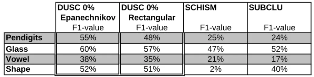
2.10 F1-value on real world data using different density measures . 61 3.1 Breadth first and depth first subspace clustering . . . 65

3.3 Multistep architecture . . . 72

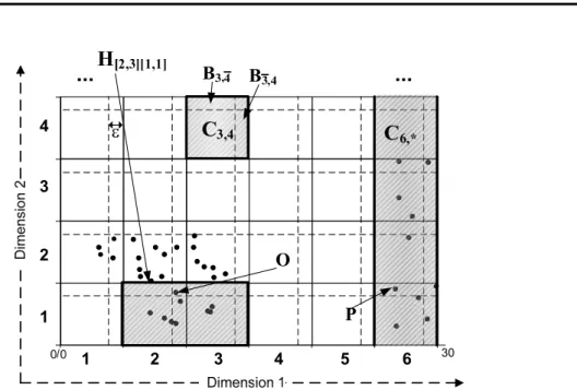
3.4 Traditional grid discretization, with connectivity borders . . . 74

3.5 Cells, connectivity borders and hypercubes projected to di-mension 1 and 2 . . . 75

3.6 Multistep eDSUC algorithm . . . 78

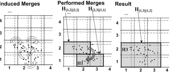
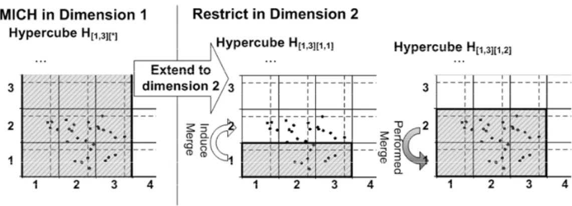
3.7 Induced and performed merges . . . 79

3.8 Extending a MICH to next dimension . . . 80

3.9 Example data set: transforming objects to cell representations 84 3.10 Creating the initial SC-tree for the example data set . . . 88

3.11 Restricting the SC-tree . . . 91

3.12 Inducing merges using the SC-tree . . . 93

3.13 Processing the next cell using the SC-tree . . . 94

3.14 Merging cells using the SC-tree . . . 95

3.15 Pruning based on the SC-tree . . . 96

3.16 SC-tree availability during mining . . . 98

3.17 Scalability vs. dimensions . . . 103

3.18 Scalability vs. database size . . . 104

3.19 Selectivity vs. dimensions . . . 105

3.20 MinPoints vs. runtime . . . 106

3.21 F parameter vs. runtime . . . 107

3.22 Gridsize vs. runtime . . . 107

3.23 Three kernels vs. SUBCLU and SCHISM . . . 108

3.24 Runtimes for sorting heuristic . . . 109

3.25 Tree size for sorting heuristic . . . 110

3.26 Redundancy . . . 111

3.27 Redundancy Quality . . . 112

3.28 Quality on real data . . . 113

3.29 Runtime on real data . . . 113

4.1 Subspace clustering overview . . . 120

4.2 Detailed view for one subspace cluster . . . 121

4.3 Bracketing redundancy in MDS images . . . 122

4.4 Matrix of subspace clusters groups . . . 123

4.5 User Interface for a Subspace Clusters Matrix . . . 125

4.6 Subspace clusters matrix for different settings . . . 126

5.2 Example pattern . . . 135

5.3 Example for a subspace subsequence cluster . . . 136

5.4 Hierarchical index structure for finding subsequence clusters . 141 5.5 Subsequence clustering algorithm . . . 144

5.6 Creating Candidate Clusters . . . 144

5.7 Transformation example . . . 146

5.8 Influence of σ on density . . . 149

5.9 Parameter guidelines . . . 150

5.10 Comparison with SUBCLU . . . 151

5.11 Scalability for number of attributes . . . 152

5.12 Scalability for sequence length . . . 153

5.13 Performance . . . 155

5.14 Cluster Visualization for river data . . . 156

5.15 Clustering of weather dataset . . . 157

Efficient density-based methods for classification 6.1 Class conditional density using naive Bayes . . . 166

6.2 Class conditional density using mixture densities . . . 167

6.3 Class conditional density using mixture densities . . . 169

6.4 Class conditional density using mixture densities . . . 170

7.1 Prototypical anytime classification accuracy . . . 176

7.2 Pruning for traditional queries and probability density queries 179 7.3 Different density estimation approaches . . . 180

7.4 R-tree, Bayes tree and mixture densities on three Bayes tree levels . . . 181

7.5 Computing mean and variance . . . 183

7.6 Nodes and Entries in the Bayes tree . . . 185

7.7 Split in the Bayes tree . . . 186

7.8 Frontier of a Bayes tree . . . 189

7.9 Bayes tree of height 2 and fanout 2 . . . 190

7.10 Probabilistic descent vs. geometric descent on synthetic data 195 7.11 Refinement strategies Order vs. Maximal . . . 196

7.12 Comparing Bayes tree on synthetic data . . . 198

7.13 Comparing Bayes tree on real world data . . . 199

8.1 Lattice of subspaces used for up- and downward pruning . . . 212

8.2 Example top down generation . . . 213

8.3 Pruning of subspace X1X2X3 . . . 214

8.4 Varying β on synthetic data . . . 216

8.5 Varying β on flight delay data . . . 217

8.6 Varying w on synthetic data . . . 218

8.7 Varying w on flight delay data . . . 218

There are many people who supported and encouraged me while I was work-ing on my thesis. At this point I would express my gratitude to all of them, even if I cannot mention everyone here.

First of all, I would like to thank my supervisor Prof. Dr. Thomas Seidl. This thesis would not have been possible without your advice, helpful dis-cussions and support. Thank you for always being interested in my work.

I am also very grateful to Prof. Dr. Bart Goethals for his time and valuable discussions. Thank you also for agreeing to review this thesis.

Special thanks also to my colleagues for the inspiring discussions and fruitful cooperations. Working in an interested and humorous team was very helpful for this thesis.

Last but not least I would like to thank my parents, family and friends. But especially I want to thank my wife Melanie for all the love and great encouragement during the last years. I would also like to thank Julia for just being there and reminding me that there exists a task more important than this work.

Today’s data storage facilities allow recording of billions of transactions from business applications, scientific sensor readings, monitoring systems etc. Sci-entists developing new drugs, system administrators monitoring complex technical processes, and decision makers being responsible for complex social or technical systems require an overview and even a deeper understanding of their respective data. The knowledge discovery in databases (KDD) process has been designed to identify hidden patterns in large data resources. A central step of the KDD process is the data mining task. Major data mining tasks are clustering and classification. Density-based approaches have proven to be very effective for many data mining methods. However, the good ef-fectiveness often comes at the cost of a high runtime complexity. This thesis presents new efficient density-based approaches for different data mining ap-plications whereas the effectiveness of the new developed methods is always kept in mind.

The first part of this thesis is concerned with new density-based cluster-ing methods. Clustercluster-ing is a data mincluster-ing task for summarizcluster-ing data such that similar objects are grouped together while dissimilar ones are separated. Density-based approaches have shown to successfully mine arbitrary shaped clusters even in the presence of noise. In multi-dimensional or high dimen-sional data, clusters are typically hidden by irrelevant attributes and do not show across the full space. As relevance of attributes is not globally uniform for all clusters, global dimensionality reduction approaches are not adequate. Subspace clustering aims at automatically detecting clusters and their rele-vant attribute projections. This work presents a new clustering model DUSC which guarantees a comparable and redundancy free subspace clustering re-sult. As the number of possible subspaces is exponential in the number of dimensions subspace clustering is a computationally challenging task. The algorithm eDUSC developed in this work is based on a filter-and-refinement

architecture which avoids repeated database scans. Further on, this work proposes a new visualization technique for subspace clusters and a special-ized clustering technique for multi-dimensional sequence databases.

The second part of this thesis proposes new density-based methods for classification. Classification aims at assigning a class label to unknown ob-jects. Various approaches for classifying objects have been investigated in the last decades. Classifiers based on statistical approaches have been most intensively studied in the literature and results like asymptotical behavior and classification bias have been derived. To apply statistical classifiers the density of objects has to be estimated. In this work, a hierarchy of density estimators is proposed which makes the classification of objects possible any-time. Additionally, a new classification method using subspace clusters for higher dimensionalities is developed in this thesis.

The proposed density-based clustering and classification methods are evaluated in terms of both efficiency and effectiveness in thorough experi-ments on real world and synthetic data.

Moderne Datenspeicheranlagen erm¨oglichen die Erfassung von Billionen von Gesch¨aftstransaktionen, wissenschaftlichen Sensormessungen, Meldungen von

¨

Uberwachungssystemen etc. Verantwortliche Wissenschaftler in der Arznei-mittelentwicklung, Systemadministratoren, die komplizierte technische Pro-zesse ¨uberwachen und Entscheidungstr¨ager komplexer sozialer oder techni-scher Systeme ben¨otigen eine ¨Ubersicht ¨uber bzw. einen tieferen Einblick in ihre erfassten Daten. Der “Knowledge discovery in databases” (KDD) Pro-zess wurde entwickelt, um versteckte Muster innerhalb großer Datenbanken ausfindig zu machen. Ein zentraler Schritt des KDD Prozesses ist das Da-ta Mining. HaupDa-taufgaben des DaDa-ta Minings sind das Clustering und die Klassifikation von Daten. Dichtebasierte Ans¨atze haben sich als sehr effekti-ve Data Mining Methoden bew¨ahrt. Jedoch bringt die hohe Effektivit¨at eine hohe Laufzeitkomplexit¨at mit sich. In dieser Doktorarbeit werden neue, ef-fiziente, dichtebasierte Ans¨atze f¨ur verschiedene Datenanalyseanwendungen vorgestellt, wobei die Effektivit¨at nicht außer Acht gelassen wird.

Der erste Teil dieser Arbeit befasst sich mit neuen dichtebasierten Clus-tering Methoden. ClusClus-tering ist eine Data Mining Aufgabe, welche Daten so zusammenfasst, dass Gruppen ¨ahnlicher Objekte von un¨ahnlichen sepa-riert werden. Dichtebasierte Ans¨atze haben sich als erfolgreich bei der Su-che beliebig geformter Cluster innerhalb verrauschter Datens¨atze herausge-stellt. In mehr- oder hochdimensionalen Daten werden Cluster normalerweise durch irrelevante Attribute versteckt und sind daher im vollen Datenraum nicht zu erkennen. Da die Relevanz von Attributen nicht f¨ur alle Cluster global einheitlich ist, k¨onnen globale Dimensionsreduktionstechniken nicht sinnvoll eingesetzt werden. Die Zielsetzung von Subspace Clustering Algo-rithmen ist das automatische Auffinden von Clustern mit der zugeh¨origen Attributprojektion. Diese Arbeit pr¨asentiert DUSC, ein neues Clustering Mo-dell, das vergleichbare und redundanzfreie Clustering Ergebnisse garantiert.

Aus Sicht des Berechnungsaufwandes stellt Subspace Clustering, wegen der exponentiellen Abh¨angigkeit der Anzahl m¨oglicher Teilr¨aume von der An-zahl Dimensionen, eine Herausforderung dar. Der Algorithmus eDUSC, wel-cher im Rahmen dieser Arbeit entwickelt wurde, basiert auf einer Filter-und-Verfeinerungsmethode, wodurch das wiederholte Durchsuchen der Datenbank vermieden wird. Weiterhin werden in dieser Arbeit Visualisierungstechniken f¨ur Subspace Cluster vorgestellt, sowie eine spezialisierte Clustering Technik f¨ur mehrdimensionale Sequenzdatenbanken.

Im zweiten Teil dieser Doktorarbeit werden neue dichtebasierte Methoden zur Klassifikation vorgestellt. Das Ziel der Klassifikation ist die Bestimmung eines Klassenlabels f¨ur unbekannte Objekte. In den letzen Jahrzehnten wur-den verschiewur-dene Ans¨atze f¨ur die Klassifikation von Objekten vorgestellt. Klassifikatoren, welche auf statistischen Ans¨atzen basieren, wurden in der Literatur sehr intensiv untersucht und Ergebnisse ¨uber das asymptotische Verhalten und die Klassifikationstendenz wurden hergeleitet. Zur Anwendung statistischer Verfahren ist das Sch¨atzen der Dichte f¨ur Objekte notwendig. In dieser Arbeit wird eine Hierarchie von Dichtesch¨atzern vorgestellt, die Klassi-fikation von Objekten zu jedem Zeitpunkt m¨oglich macht. Weiterhin wird in dieser Doktorarbeit ein neuer Klassifikator f¨ur hochdimensionale Daten auf Basis von Subspace Clusterings entwickelt. In umfangreichen Experimenten wird mit Hilfe von synthetischen und realen Daten sowohl die Effizienz als auch die Effektivit¨at der vorgestellten dichtebasierten Clustering- und Klas-sifikationsmethoden untersucht.

knowledge discovery in

databases

databases

Increasingly large data resources in life sciences, mobile information and com-munication, e-commerce, and other application domains require computer-based techniques for gaining knowledge. More and more data are produced by sensor networks, technical or financial monitoring systems, scientific ex-periments, or telecommunication networks. For decision makers, scientists and other data analysts unknown dependencies in the observed measure-ments are crucial for development of new models that detect and explain causalities. Knowledge discovery in databases aims at generating novel and interesting information hidden in the data [HK01]. To find interesting pat-terns in a data set a knowledge discovery process is typically divided into four steps (see also Figure 1). The first step creates a consistent view on the data by integrating and cleaning data stored in different sources. The combined data is often managed in a data warehouses. Depending on the desired analysis the task relevant data is selected from the data warehouse or

?

?

…

Clustering

clustered data set unlabeled data set

Figure 2: Clustering a data set

transformations and projections are calculated. Subsequently the data min-ing step extracts patterns from the task relevant data. Finally visualization techniques are used to present the extracted patterns to the user.

As a central step of the KDD process the data mining step has attracted much attention from scientific research. Typical data mining approaches are association rule mining, clustering and classification methods. Clustering and classification methods are often used to analyze multi-dimensional real valued data sets. Common subtasks of many clustering or classification algorithms are density-based (i.e. they rely on densities of regions or objects). Since databases tremendously grow in size classification and clustering algorithms have a special need for efficient density-based methods.

Density-based methods for clustering

Clustering aims at grouping data into similarity-based subgroups. Typically clustering methods do not assume any prior knowledge, i.e. the number of groups contained in the data or the type of clusters is unknown. Consequently clustering methods are often called unsupervised. Figure 2 gives an abstract example for a clustering. In this example the given data set is grouped into three regions.

In the literature, several clustering paradigms exist [HK01]. Density-based clustering defines clusters as dense areas separated by sparsely pop-ulated areas. It has been shown to successfully detect clusters of arbitrary shape in many settings [EKSX96, HK98]. Density of an object is measured either by mere counting of objects or by more complex functions on the number and location of objects in the neighborhood. The underlying

den-sity model, from mere counting of objects in a neighborhood range to local density attractors, has great impact on the clustering result.

For any paradigm, clustering in high dimensional spaces is obstructed by the noise of irrelevant attributes. The “curse of dimensionality” describes the effect that distances become more and more similar as dimensionality increases. Consequently, meaningful clusters no longer exist [BGRS99].

One solution for clustering data in multi-dimensional or high dimensional spaces is subspace clustering. In scenarios with many attributes or with noise, clusters are often hidden in subspaces of the data and do not show up in the full dimensional space. A global reduction to relevant attributes is often infeasible, as relevance of attributes is not necessarily globally uniform. Varying relevance of attributes for individual clusters requires clustering over any possible subset of the attributes.

Subspace clustering therefore aims at detecting clusters in any possible attribute combination. Density-based approaches are very popular to deter-mine clusters in subspace. As the number of subspace projections is exponen-tial ly with the number of dimensions, subspace clustering methods have a tremendous need for efficient density-based methods. We will go into details of subspace clustering in Part I.

Density-based methods for classification

Classification methods aim at assigning unlabeled objects to predefined groups. As the number of groups are known in advance classification methods are calledsupervised methods. Many applications have the need to predict class labels for new objects like speech and image recognition systems, e-mail spam and denial of service attacks detection systems etc. Since an a priori knowl-edge about the classes is given the goal of a classifier is to learn the structure of the predefined groups from a given labeled data set (the training data). Figure 3 illustrates an abstract concept for a classifier which learns the prede-fined classes from dense regions (different classes are represented by different colors).

Using statistical classifiers is a popular approach in pattern recognition system [DHS01]. Many of these methods are based on density estimations (e.g. the Bayes classifier). As the density distribution of the data is typically not known in advance densities are estimated from the training set. A typical

learned classifier labeled data set

Figure 3: Classifier learned from data set

approach is to estimate the missing parameters of a density model from the training set (e.g. estimate mean and variance for a Gaussian distribution). However, assuming a concrete model is often not appropriate as many density models are unimodal which is a too strong constraint especially for multi-dimensional data sets. Mixture models relax the assumption of one concrete model by using a multimodal mixture of densities. A popular solution is to use an expectation maximization (EM) algorithm to learn a mixture of Gaussian densities from the training set.

Nonparametric functions on the other hand can be used for arbitrary dis-tributions as they make no assumption about the form of the distribution. Kernel densities (or parzen windows) are nonparametric functions which es-timate the density of a query object directly from the distribution of the objects contained in the surrounding region. Kernel densities have proven to be an effective method for many applications. However, as the distribution for each query-region has to be determined from the training objects the effi-ciency of kernel estimators is often poor. In Part II we present details about efficient density-based methods used for classification.

Outline of this work

In this work we present new efficient density-based methods for various clus-tering and classification applications. The thesis is divided into two major parts:

Part I is concerned with new density-based clustering methods.

InChapter 1 we discuss clustering of multi-dimensional data. We further on give an overview over existing clustering methods and discuss problems

oc-curring in multi-dimensional or high dimensional data sets. We then present existing solutions for finding clusters in projections of the data and present preliminary definitions for density-based clustering in subspaces.

Existing subspace clustering methods ignore an effect we call dimension-ality bias. Chapter 2 formalizes this effect and proposes a new subspace clustering model DUSC which solves this problem. Additionally to dimen-sionality bias the redundancy of clusters is evaluated in thorough experiments on synthetic and real world data sets.

As the number of possible subspaces is exponential in the number of dimensions, subspace clustering is a computationally challenging task. In Chapter 3 we develop an efficient method eDSUC for our DUSC subspace clustering method. eDUSC achieves a high efficiency by using a filter-and-refinement architecture for avoiding computational intensive database scans. Based on a depth-first algorithm eDUSC exploits in-process redundancy pruning as well as indexing dense regions. Comparing eDUSC with state-of-the-art subspace clustering methods proves the efficiency and effectiveness of this approach.

An important step of the KDD process is to visualize the result of the data mining method to the user. Visualizing the result of subspace cluster-ing algorithms is no trivial task as structures contained in different possible overlapping subspaces have to be presented to the user. The VISA approach presented in Chapter 4 proposes two new visualization techniques for sub-space clusterings.

Chapter 5 proposes a specialized subspace clustering technique for an-alyzing databases of multi-dimensional sequences which was developed in collaborations with hydrologists. In a current project of the German govern-ment different structural quality measures for more than hundred thousand river segments have been recorded. The special challenge in this project was to develop a subspace clustering method for finding clusters of arbitrary sequence length and in any subset of the attributes. The efficiency of the new clustering model is guaranteed by using a two phase approach utilizing different monotonicity properties.

Part II is concerned with new density-based classification methods: In Chapter 6we give a brief review over existing classification algorithms proposed in the literature. Further more the basic notations of the Bayes and nearest neighbor classifier are presented in this chapter.

objects at any point in time is developed in Chapter 7. A novel hierarchy of densities for different classes (the Bayes tree) is exploited for efficient classification. We evaluate the accuracy of our Bayes tree for varying stream inter-arrival rates on synthetic and real world data sets.

Chapter 8proposes a new classification technique which incorporates the information the class distribution into a specialized subspaces clustering al-gorithm. Classification based on these classifying subspace clusters exploits both class and local correlation information. In collaboration with a local company optimizing airport scheduling purposes we investigate the classifi-cation accuracy of flight delays.

Finally we summarize the major contributions of this work and give an outlook on future research direction.

Efficient density-based methods

for clustering

Clustering multi-dimensional

data

To gain insight into large data resources, data mining provides automatic techniques to extract information from large databases. One of the major tasks for knowledge discovery in databases is clustering. Clustering aims at grouping data such that objects within groups are similar while objects in different groups are dissimilar.

Many different paradigms for clustering data sets have been proposed in the last decades. We first give a brief overview over traditional cluster-ing methods in Section 1.1 before we discuss challenges in clustercluster-ing multi-dimensional and high multi-dimensional data (see Section 1.2). We then review existing solutions for clustering multi-dimensional data in Section 1.3. Sub-sequently we give the basic definitions for density-based subspace clustering. As clusters in higher dimensional spaces are often blurred by noise subspace clustering algorithms identify clusters in any possible subspace. In the fol-lowing chapters of this part we will discuss different aspects of density-based subspaces clustering.

1.1

Full-space clustering

Traditional clustering methods use all attributes available to identify clusters contained in the data. Hence, we refer to traditional clustering methods which do not consider lower dimensional projections of the data as full-spaces clustering methods.

One of the first approaches proposed in the literature to cluster a data set is partitioning clustering. As their name suggests, partitioning clustering methods create a disjoint grouping of the data. Typically they iteratively improve an initial partition of the data until a cost function converges. A well-known example is the k-means algorithm [Mac67], or more statistically founded, EM (Expectation Maximization) [Lau95]. Partitioning algorithms are limited to the detection of convex clusters in data without noise where the number of clusters is known in advance.

As the number of clusters is often not known, hierarchical clustering meth-ods do not determine one unique clustering structure but a hierarchy of clus-ters. Two different approaches for hierarchical clustering methods can be distinguished: divisive (top-down) and agglomerative (bottom-up) methods. Divisive methods start with a single cluster that contains all objects and recursively pick one cluster for splitting [JD88]. Agglomerative methods first assign each object to an individual cluster and then respectively link the two closest clusters together w.r.t. a chosen distance function. Different distance functions for agglomerative clusterings have been proposed in the literature [Sib73, Def77]. To visualize a hierarchical clustering, dendrograms represent the clustering in a tree-based organization. Each leaf node of the dendrogram corresponds to one object. Inner nodes represent clusters which contain all objects of the leaf nodes of the respective subtree. In each level the two closest clusters are linked together. By choosing different levels in the dendrogram users obtain different groupings of the objects. As no concrete clustering is mined by hierarchical clustering algorithm it is often difficult to extract hidden structures contained in the data based on the clustering result. Hence, visualization techniques like dendrograms are crucial to comprehend the hierarchy of clusters mined by hierarchical clustering algorithms.

Density-based algorithms are capable of detecting arbitrarily shaped clus-ters and have proven to work remarkably well in noisy settings. The basic idea is that clusters are dense areas separated by sparsely populated areas as defined in DBSCAN (Density-Based Spatial Clustering of Applications with Noise) [EKSX96, HK98]. The initial definition of density has been shown to oversimplify the model of the real density distribution. Fixed neighborhoods of a pre-given ε-range are checked whether or not they contain the defined minimum number of points, thus the distribution of objects is ignored and sensitivity to parameter settings is a challenge. DENCLUE (Density Cluster-ing) thus extends DBSCAN using influence functions to model local densities

of objects [HK98]. Due to efficiency considerations, an approximate compu-tation of density is used. The recent approach of DENCLU2 speeds up the density estimation by a hill-climbing approach with an adjustable step size [HG07]. A hierarchical clustering based on densities instead of distances has been proposed by OPTICS [ABKS99]. OPTICS visualizes a hierarchy of connected clusters by computing a density plot. We extend density-based clustering methods to subspace projections in the next sections.

1.2

Problems for clustering multi-dimensional

data

For any clustering paradigm, full space clustering algorithms do not scale to higher dimensional spaces. They suffer from the so called “curse of di-mensionality”. For clustering this means that clusters do not show across all attributes as they are hidden by irrelevant attributes or blurred by noise.

Clustering methods are typically either based on distances (like partition-ing and hierarchical clusterpartition-ing) or on densities (like density-based methods). The effects of higher dimensional spaces on distances and density distribu-tions have been widely studied in the literature. In [BGRS99] the authors study the effects of high dimensions on the nearest neighbordmin(o) and the

farthest neighbor dmax(o) of an object o in detail. They have proven the

following equation for different distributions:

∀ε≥0 :limdim→∞P(dmax(o)<(1 +ε)dmin(o)) = 1

This statement formalizes that with growing dimensionalities (dim) the distance to the nearest neighbor is nearly equal to the distance to the farthest neighbor (distances become more and more similar). Consequently, cluster-ing methods based on distance functions have problems to extract meancluster-ingful patterns in high dimensional spaces as they either cluster only one object (the nearest neighbor) or nearly the complete data set (the farthest neighbor).

Densities also suffer from the “curse of dimensionality”. In [Sil86] the au-thors describe an effect of higher dimensions on density distributions: 99% of the mass of a ten-dimensional normal distribution is at points whose distance from the origin is greater than 1.6. This effect is directly opposite in lower dimensional spaces: 90% of the objects have a distance of less than 1.6 from

0 0.1 0.2 0.3 0.4 0.5 0.6 0.7 0.8 0.9 1 0.0 0.4 0.8 1.2 1.6 2.0 2.4 2.8 3.2 3.6 4.0 1‐dimensional normal  distribution 2‐dimensional normal  distribution 10‐dimensional normal  distribution 20‐dimensional normal  distribution

1-dimensional standard normal distribution

2-dimensional standard normal distribution

Radius of sphere

Probability

Figure 1.1: Probability of different standard normal distributions

the origin regarding a one-dimensional distribution.

We additionally illustrate the behavior of higher dimensional standard normal distributions in Figure 1.1. For different dimensionalities we mea-sured the probability of an object to be contained in a sphere positioned at the origin w.r.t. the radius of the sphere. On the right part of the figure the probability is graphically illustrated for a sphere of radius 1.6 for a one and two-dimensional standard normal distribution (the corresponding prob-abilities are marked by red points in the graph). Please recall that density functions are normalized to one and hence the volume of a region under a density function corresponds to the probability of that region. As we can see the probability for an object to be contained in the center of a space is drop-ping extremely for higher dimensions. In a 20-dimensional space most of the objects have a distance of more than four times the variance per dimension. Consequently nearly every point is positioned at the border of the data space even though the highest density of a high dimensional normal distribution is still at the origin. Density-based clustering methods hence have problems to determine the density of a region as the objects are scattered over the data space.

One possible approach to clustering high dimensional data sets is to apply dimensionality reduction techniques in advance. After reducing the dimen-sionality clusters can be identified. Dimendimen-sionality reduction techniques like PCA (principle components analysis) aim at discarding irrelevant dimensions [Jol86]. However, in many practical applications, no globally irrelevant

di-0 1 2 3 4 5 6 7 8 0 1 2 3 4 5 6 7 8 0 1 2 3 4 5 6 7 8 0 1 2 3 4 5 6 7 8 Dimension x3 Dim ension x 4 0 1 2 3 4 5 6 7 8 0 1 2 3 4 5 6 7 8

Data set clearly containing four clusters in dimension one, two (colored respectively)

No clustering structure visible in dimension one,three Dimension x1 ion x 2 Dimension x1 nsion x 3

Different clustering structure shows up in dimension three, four

0 1 2 3 4 5 6 7 8 0 1 2 3 4 5 6 7 8

No clustering structure visible in dimension two,three

Dimension x2

Dime

nsion x

3

Figure 1.2: Problems of dimensionality reduction and projected clustering techniques

mensions exist. Thus, for these settings, dimensionality reduction can only discover a subset of the actual clusters as some of the original dimensions are ignored.

Figure 1.2 gives an example for a 4-dimensional data set containing clus-ters in different projections. We illustrate four different projections of the data set in Figure 1.2 (to dimensions x1x2, x1x3, x2x3 and x3x4). As

de-picted clusters are clearly visible in two different projection (x1x2 and x3x4).

Since each of the four dimensions is relevant for some clusters globally ir-relevant dimensions do not exist. Hence, removing dimensions will discard

some cluster: e.g. if dimension x3 and x4 are removed in advance the four

clusters contained in the projection x1x2 can be identified by a clustering

algorithm (upper left part of Figure 1.2). As we can see dimension x3 is

irrelevant for this clustering as both projections to dimensionsx1x3 and x2x3

does not contain any clusters (see upper right and lower left part of Figure 1.2). However, if dimension x3 is removed the clustering structure obtained

by projecting the data to the dimensions x3x4 is lost. Hence, dimensionality

reduction techniques can not be applied without loss of clusters. Further on, both clustering structures contained in this example are distorted if all four dimensions are considered. Consequently using a full-space clustering method is also not appropriate for this example data set.

1.3

Solutions for clustering multi-dimensional

data

As discussed in the last section finding structures in multi-dimensional to high dimensional spaces is problematic due to the curse of dimensionality. However, clusters still exist in lower dimensional projections. Specialized clustering algorithms have been developed in the last decade which identify clusters in subspaces of the data space. Many traditional clustering algo-rithms have been extended to projected or subspace clustering algoalgo-rithms. Methods for identifying clusters in subspaces can be categorized into top-down and bottom-up methods or into projected and subspace methods. We discuss the two algorithmic concepts of top-down and bottom-up methods before we present different projected and subspace clustering models in the next section. In this thesis we will concentrate on subspace clustering meth-ods.

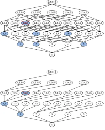
The “top” and “bottom” of top-down and bottom-up methods refer to the lattice of subspaces. Figure 1.3 presents the lattice for a five-dimensional space. At the top the full-dimensional space containing all for dimensions is illustrated (using the index set (1,2,3,4,5)) and the empty space at the bottom, accordingly. Each level in the lattice contains all subspaces of a specific dimensionality. Two subspaces are connected if they only differ in one dimension. Bottom-up methods start at the bottom of the lattice (with one-dimensional spaces) and iteratively join subspaces to higher 3dimensional subspace. To prune the search space bottom-up methods typically use

clus-o p -D o w n B o t t o m -u p

Figure 1.3: Lattice of subspace clusters

tering models which implement the downward closure property [KKZ07]. For density-based methods the density threshold has to be fixed to ensure the downward closure of clusters or subspaces. This assumption is often a problem as it leads to incomparable clustering results. We will discuss these effects in Chapter 2 in detail.

Top-down methods start by evaluating the full-dimensional space. In each step the current clustering result is refined by projecting individual clusters to lower dimensional spaces. The local neighborhood of a cluster in the high dimensional space is commonly used to determine the lower dimen-sional projection [KKZ07]. The quality of top-down methods often depends on the quality of the initial clustering in the full-dimensional space. Since clustering multi-dimensional data sets is often problematic projected clus-tering algorithms do not scale well to higher dimensional data. Further on, starting in high dimensional spaces is also not unproblematic as we discussed in the last chapter (see “curse of dimensionality”).

1.3.1

Projected clustering

One approach to find clusters in multi-dimensional data sets is projected clustering. Projected clustering methods identify projections of the data into lower dimensional spaces where disjoint clusters may be identified. Projected clustering algorithms try to identify the relevant dimensions for each cluster individually. Typical projected clustering approaches extend partitioning

clustering methods by computing the relevant dimensions for each cluster. PROCLUS (PROjected CLUStering) [AWY+_{99] extends the k-medoid}

algorithm by iteratively refining a full-space k-medoid clustering. Hence, PROCLUS works in a top-down manner. In each iteration the clusters are projected to a lower dimensional axis-parallel subspace and the data points are reassigned to their closest medoid.

ORCLUS (arbitrarily ORiented projected CLUSter generation) extends PROCLUS by using arbitrary projections for each cluster [AY00]. Both algorithms need the number of clusters and the (average) dimensionality of the clusters as input parameter.

LAC (Locally Adaptive Clustering) [DPGM04] weights the dimensions for each cluster by measuring the variance. The reassignment of points is based on the k-means approach and like ORCLUS and PROCLUS LAC starts with an initial full-space clustering before the individual weights per dimension are computed. The influence of the variance on the weight of a dimension is controlled by a user specified parameter.

Recently P3C (Projected Clustering via Cluster Cores) has been proposed [MSE06]. P3C works in a bottom-up manner by combining one-dimensional cluster cores to higher dimensional clusters. By using these cluster cores as an initialization for the EM algorithm, a partitioning is computed. As discussed before, clusters may overlap in different projections, and hence these approaches cannot detect all clusters.

Projected clustering algorithms are not able to find different clustering in overlapping subspaces. Reconsider the example data set presented in Figure 1.2. Since projected clustering algorithms only detect one clustering one of the two structures contained in this example would not be found. Hence, projected clusterings also lose some clusters if clusters are hidden in different projections.

1.3.2

Subspace clustering

To identify clusters in different projections subspace clustering methods aim at detecting clusters in any subspace. In principle, any clustering algorithm could be used to mine clusters in all subspaces of the data. This naive ap-proach is of very high complexity as the number of subspaces is exponential in the number of dimensions and the result size is typically overwhelming. Consequently, subspace clustering approaches have largely focused on

reduc-Subspace

Clustering

Search

Grid

Density

Grid

_Density

based

based

based

y

based

Figure 1.4: Categorization of existing subspace clustering concepts

ing the search space via heuristics, discretization of the data space via grids, etc. Another approach to efficiently compute subspace clusters is to search for relevant subspaces prior to clustering. A categorization of the different approaches is given in Figure 1.4.

Grid-based

CLIQUE (Clustering In QUEst) is the first subspace clustering method pro-posed in the literature. CLIQUE uses a grid to discretize the search space [AGGR98]. Monotonicity on the density of grid cells is used for pruning the search space in a bottom-up algorithm. Grids greatly reduce the compu-tational complexity, yet clusters which spread across several cells might be missed. Moreover, CLIQUE measures density via simple counting of objects per cell. MAFIA [NGC99] extends CLIQUE via a data-adapted grid to re-duce the number of clusters lost in discretization. Density is then computed depending on the size of a cell.

DOC and its variant FastDOC [PJAM02] are not directly based on a grid like discretization but define subspace clusters as dense hypercubes of a user defined size. The relevant dimensions for a subspace cluster are selected by using a Monte Carlo algorithm. An optimal subspace cluster is then defined by taking the number of points and the dimensionality of the subspace into account. Since clusters are defined using cells, clusters might also be cut apart. Further on, the density of arbitrarily shaped clusters is only

approximated by the hypercube as the actual distribution of points is not considered.

SCHISM (Support and Chernoff-Hoeffding bound-based Interesting Sub-space Miner) [SZ04] extends CLIQUE using a variable threshold to cope with different dimensionalities, yet relies on heuristics and a grid-based discretiza-tion for pruning. Consequently, completeness is lost as in all grid-based approaches.

Density-based

Density-based clustering has been extended to subspace clustering in previous works. SUBCLU (density-connected Subspace Clustering) uses a gridless approach for effective subspace cluster mining [KKK04]. Using the earlier DBSCAN density notion, a density monotonicity property is used to prune subspaces. The algorithm uses an apriori like scheme (discussed first in association rule mining [AS94]) to detect subspace clusters in a bottom-up fashion. As dimensionality is ignored, it suffers from dimensionality bias, i.e. clusters cannot be separated from noise across subspaces (see also Chapter 2).

FIRES [KKRW05] is a generic framework for subspace clustering which allows using different clustering notions. It relies on approximative tech-niques in a filter-refinement scheme to scale to high dimensional spaces.

Subspace search

As mentioned above, faced with the huge number of subspace clusters differ-ent heuristics are used to efficidiffer-ently determine subspace clusters. Subspace search methods use a two step approach. The first step searches for subspaces having a high cluster tendency. These subspaces are typically ranked using a scoring function. Actual subspace clusters are determined in a second step using traditional clustering methods.

ENCLUS [CWZZ99] (Entropy-Based Subspace Clustering) discretizes the data to compute the entropy and information gain of a subspace. Working bottom-up one-dimensional subspaces are evaluated first and then combined to higher dimensional subspaces. Entropy and information gain thresholds are used to prune the search space. The result is then clustered using a grid-based method like CLIQUE. An extended version of ENCLUS uses a

normalized entropy measure and an evolutionary approach to identify sub-spaces having a high cluster tendency [AKSS06].

RIS [KKKW03] (Ranking Interesting Subspaces) uses a density-based method to determine the interestingness of a subspace. Subspaces are ranked according to their ratio of actual and expected number of dense objects (core objects). Clusters are then mined using a density-based algorithm.

As subspace search methods do not mine the actual subspace clusters, the scoring function for subspaces does not necessarily reflect the differences in clusters contained:

1.4

Basic notions

In this section, we give the formal definitions for density-based subspace clus-tering as used in our algorithmic concepts. Density-based subspace clusclus-tering algorithms identify arbitrarily shaped clusters in multi-dimensional feature databases. For notational convenience let us first introduce some basic no-tions:

Definition 1.1 Preliminary Definitions

We assume mining clusters in a data set based on the following definitions. Given:

• a d-dimensional feature space with the corresponding index set D =

{1, . . . , d}

• a universal domain U= [0,v] for all dimensions

• a database DB⊆U|D| containing |DB|=n objectso = (ν1. . . νd)

we define projections of data objects onto different subspaces based on:

• the index set of a subspace asS ={s1, . . . , sr} ⊆D

• a subspace U|S| as the projection of U|D| to the r dimensions specified by the index set S

• DB|S| as the projection of DB|D| to the dimensions in S

• a projection of object o = (ν1. . . νd) to the subspace U|S| as oS =

In density-based clustering, clusters are defined as dense areas separated by sparsely populated areas. Hence, a basic definition for density-based clustering is a density measure which can be evaluated for every object. Usually the density value is determined by considering an area of influence surrounding the data object. This area of influence is specified using a norm

k.k and a parameterε which defines the radius of the area: Definition 1.2 Area of influence

The area of influence Aε for a given norm k.k

kok:U|D| → R

and a parameter ε is defined as:

Aε(o) ={p | p∈DB,kp−ok ≤ε}

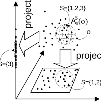
As mentioned before, in many applications clusters are hidden in sub-spaces and cannot be revealed by any cluster analysis that mines all dimen-sions simultaneously. Subspace clustering methods, on the other hand, aim at detecting clusters by automatically focusing to the respectively relevant subsets of the dimensions.

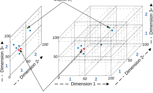
Hence, for subspace clustering it is essential that the density measure is capable of handling objects of different dimensionalities (see also Figure 1.5). In [KKK04] the standard notion of density is extended for the evaluation of subspaces. Following the paradigms of subspace clustering we extendk.k to

k.kS _{by restricting the norm k.k : U}|D| _{→ R to the dimensions in subspace}

S. For ease of notation, we refer to a subspace U|S| only by its index set S. As a result, we obtain an adapted notion of the area of influence as the (S, ε)-neighborhood. Figure 1.5 illustrates the projection of the area of in-fluence for objecto onto two different subspaces (S={1,2} and S={3}).

Definition 1.3 Subspace area of influence

The area of influence AS

ε in a subspace S and the respective norm k.k S kokS =oS :U|S|→ R is defined as: AS ε(o) ={p | p∈DB,kp−ok S _≤ε}

A

projection

projection

S={1,2,3}

S={1,2}

S={3}

Figure 1.5: Projection and area of Influence

In density-based clustering, an object o is defined as dense if its density exceeds a threshold τ. Typically, density of an object o is determined by simply counting the number of objects in AS

ε(o). We generalize this idea

by assigning weights to each object contained in AS

ε(o). This is depicted in

Figure 1.6: the left neighborhood range shows a different distribution than the one on the right, even though both contain the same number of objects. By assigning less weight to objects further away, this effect is modeled in the density definition. Based on a monotonously falling weighting function W :R → R we define a density measure as:

Definition 1.4 Generalized Density Measure

Let W be an arbitrary weighting function W : R → R. Based on W a generalized density measure ϕS

ε(o) for an objecto in subspace Sis defined as:

ϕS_ε(o) = X

p∈AS

ε(o)

W kp−okS

Using a weighting function W a density measure ϕS_ε(o) weights the ob-jects within the neighborhood according to their distance from the object

Figure 1.6: Density distribution within neighborhood

o. Consequently, an object o in subspace S is called dense if the weighted objects contained in its area of influence sum up to more than a given den-sity threshold τ. The weight of an object contained in the area of influence is determined by a norm which reflects the distance of the object from the point of evaluation.

Definition 1.5 Subspace Density-Connected.

An object o is dense in subspace S (S-dense) with respect to the area of influence ε if its density exceeds the density-threshold τ:

S-denseτ_ε(o) ⇔ ϕS_ε(o)≥τ

A subsetC⊆DBis connected with respect to a subspaceS(S-connectedC)if

there is a chain of neighboring objects between all pairs of objects (p, q)∈C:

∀(p, q)∈C : S-connectedC(p, q) ⇔

∃ o1. . . on∈C:

o1 =p, on=q ∧

∀ i= 1. . . n−1 :koi−oi+1kS ≤ε.

A density-based cluster is then defined as the transitive closure of all dense connected objects, i.e. the maximal set of objects which are density-connected. Clusters thus are elements of chains of objects which are mutually included in one another‘s neighborhoods. Consequently, arbitrarily shaped clusters can be successfully detected even in noisy settings [EKSX96]. Definition 1.6 Density-based Subspace Cluster

Let U be a domain, S ⊆ D be an index set denoting a subspace US of UD. A subspace cluster (C,S)is a set of objects C⊆DBfor which the following holds:

Figure 1.7: Density-based clustering

• All objects in C areS-dense:

∀o∈C: S-denseτ ε(o)

• All objects in C areS-connected ∀p, q ∈C:S-connectedC(p, q)

• Cluster S is maximal in subspace S

∀p∈DB:S-denseτ_ε(p)∧(∃q∈C:S-connectedC(p, q))⇒p∈C

Definition 1.6 introduces subspace clusters as maximal density-connected sets of objects with respect to a subspaceS of the universeUS. Let us note that an individual objectomay belong to different subspace clusters (C1,S1)

and (C2,S2). This does not contradict maximality as long as the clusters

focus on different subspaces S1 6= S2. If an object is not contained in any

subspace cluster (Ci,Si) the object is termed noise.

SUBCLU [KKK04] first introduced the extension of the density-based clustering model of DBSCAN [EKSX96] to subspaces. In each subspace, objects must contain a minimal number of objects in its area of influence to be defined as core objects (to be dense). Similar to DBSCAN, SUBCLU distinguishes between core objects and border objects. Border objects may belong to multiple clusters, even in the same subspace, while core objects define the area belonging to a cluster.

Our definition of density generalizes the idea of core objects to dense objects with respect to a subspace S and a threshold τ. In SUBCLU all

1d cluster

1d cluster

1d cluster

2d cluster

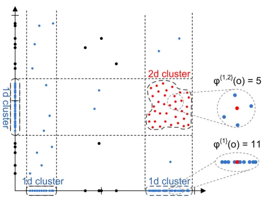
φ

(o) = 5

φ

(o) = 11

Figure 1.8: Density-based Subspace Clusters objects in AS

ε(o) are assigned the same weight: W(x) = 1,∀x ∈ R. Hence,

to determine the density of an object the number of points contained in the area of influence is counted. Thus an object is termed dense if more than τ =minP oints objects are contained in area of influence. To determine the area of influence SUBCLU uses the Euclidean distance. As this is a common approach we also focus on the Euclidean norm, but other norms could be used as well: kp−okS = s X i∈S (pi−oi)2

Figure 1.8 illustrates a basic subspace clustering scenario. Clusters i.e. dense regions are identified in all possible subspace. In this example four different subspace clusters are identified. The area of influence surrounding an object is determined by a norm. E.g. in SUBCLU object o would be determined as dense in subspace S={1,2} if the density threshold τ is set to 5 or less (see Figure 1.8). Table 1.1 summarizes our notations.

v the maximal possible value for all domains U a universal domain U= [0,v] for all dimensions D the complete data space D ={1, . . . , d}

S a index set of a subspace S={s1, . . . , sr} ⊆D

DB the database containing n objects: DB⊆U|D| o an objectso ∈DBwith d attributes o = (o1, . . .d)

oS _{projection of objectso to subspace S:o = (o}

1, . . . , od)

kokS the norm of an object o in subspace S

W(x) a weighting function for x∈ R

ε the parameter specifying the size of the area of influence

AS

ε(o) the objects contained in the area of influence of object o

in subspace S ϕS

ε(o) a density measure for an object o based on a weighting function W,

a normk.k and the respective area of influence AS ε(o)

τ the threshold parameter for the density measure: gd(o)≥τ Table 1.1: Notation for subspace clustering

Unbiased density-based

subspace clustering

As discussed in the last chapter, in scenarios with many attributes or noise, clusters are often hidden in subspaces of the data and do not show up in the full dimensional space. For these applications, subspace clustering methods aim at detecting clusters in any subspace. Existing subspace clustering ap-proaches fall prey to an effect we call dimensionality bias. As dimensionality of subspaces varies, approaches which do not take this effect into account fail to separate clusters from noise.

In this chapter, we focus on eliminating the dimensionality bias. We give a formal definition of dimensionality bias and analyze consequences for sub-space clustering. A new density-based subsub-space clustering approach (DUSC) based on statistical foundations is proposed which takes the dimensionality of the respective subspace into account. We show that this method elimi-nates dimensionality bias and leads to comparable clustering results between subspaces of different dimensionalities. In thorough experiments on syn-thetic and real world data sets, we demonstrate that our new dimensionality unbiased subspace clustering models clearly outperforms existing subspace clusterings in terms of accuracy.

2.1

Introduction

Density-based clustering algorithms are capable of detecting meaningful pat-terns in many applications. As described in the last chapter the density-based

clustering paradigm has been extended to subspaces clustering in previous work. However, the straight forward extension of density estimators to sub-spaces ignores the dimensionality of the investigated subspace.

In this chapter, we prove that density measures which ignore the dimen-sionality of the subspace are biased. Assuming a simple setup of uniformly distributed data, we show that biased density measures cannot distinguish this pseudo-cluster scenario from true clusters in all subspaces. As a conse-quence, dimensionality bias means failing at the very core of density-based subspace clustering. We demonstrate that existing dimensionality indepen-dent approaches check incomparable density values against the same constant threshold. Hence, these approaches fail from separating clusters from noise. Depending on the setting of the fixed density threshold existing subspace clustering algorithms either lose clusters or detect numerous pseudo-clusters. These effects have serious consequences for the quality of the result.

Summing up, our contributions include:

• definition and analysis of dimensionality bias and its consequences for subspace clustering

• definition of density-based clustering on statistical foundations

• dimensionality unbiased subspace clustering model

This chapter is structured as follows: we shortly review density measures of existing subspace clustering algorithms in the following section. Then, in Section 2.3, we discuss dimensionality bias. A novel model of density-based subspace clusters is defined. We demonstrate that this definition perfectly eliminates dimensionality bias. Analysis of our model is exploited to derive powerful pruning properties which do not jeopardize accuracy. We demon-strate the usefulness and effectiveness of our approach in thorough experi-ments on both synthetic and real world data sets in the experiexperi-ments Section 2.7.

2.2

Related work

In this section we shortly review the density measures of exiting cluster-ing methods. Many existcluster-ing subspace clustercluster-ing algorithms do not adapt the density model to the dimensionality. For example, CLIQUE [AGGR98]

partitions the data space into equi-width cells and computes the number of objects per cell. A cell is dense if it contains more than a specified number of objects. This is biased as the ratio of the volume of cells to the overall vol-ume decreases exponentially with the dimensionality. Similar cluster models have been used in MAFIA [NGC99], CBF [CJ02] and DOC [PJAM02]. All methods use a dimensionality independent threshold to determine if a cell is dense.

As mentioned in the last chapter, SUBCLU [KKK04] determines the density of an object by counting the number of objects contained in the ε-neighborhood. As objects in higher dimensional spaces are more spread out, virtually no high dimensional clusters are found.

Simply comparing the density of subspaces of different dimensionalities according to the same density measure ignores the effect of dimensionalities on density. The higher dimensional the subspace, the lower its expected density. More precisely, evaluating a set of objects in a higher dimensional subspace far less likely to be found a density-based cluster. This must be taken into account when defining a density measure for subspace. Two recent approaches, FIRES [KKRW05] and SCHISM [SZ04] use dimensionality de-pendent density measures, yet do not overcome dimensionality bias. FIRES uses an approximation to combine one dimensional clusters to high dimen-sional clusters. SCHISM uses heuristics to prune low dimendimen-sional subspace clusters and computes approximate densities on a per-cell basis.

Projected clustering algorithms typically take the dimensionality of the subspace into account but do not analyze the effect of different dimension-alities on the clustering result. PROCLUS [AWY+99] for example measures the segmental Manhattan distance (the distance relative to the number of dimensions) between an object and the center of a cluster. ORCLUS [AY00] measures the projected energy of a clustering which also considers the dimen-sionality of a subspace. P3C [MSE06] uses a Poisson threshold which depends on the dimensionality of the investigated subspace. However, no clustering algorithms investigate if the clusterings from different dimensionalities are comparable.

2.3

Dimensionality bias

Subspace clustering methods analyze data spaces of different dimensionali-ties. Consequently, avoiding an effect which we call dimensionality bias is an important issue. Dimensionality bias refers to a dependency of density on the dimensionality of the subspace: as dimensionality increases, average distances between objects increase and cluster radii grow. At the same time, the expected density within the area of influence drops accordingly. Thus, ignoring the dependency of density on the dimensionality of the subspace leads to incomparable density values.

Incomparable density values pose the following problem: the high dis-crepancy in density scales of low dimensional or high dimensional subspaces makes it impossible to find a suitable parameter for a fixed density threshold τ. If on the one hand τ is parameterized such that high dimensional clusters with low expected density are detected then numerous excess pseudoclusters are generated in low dimensional spaces where expected density is high. On the other hand, a parameterization of τ which separates clusters from noise in low dimensional spaces loses clusters in high dimensional spaces.

We call a density measure to be dimensionality unbiased if the expected density value of the density measure is independent of the dimensionality of the subspace. Statistically speaking, this corresponds to the same ex-pected density value regardless of the dimensionality of the subspace. For a generalized density measure as proposed in Definition 1.4 this statement is formalized as:

Definition 2.1 Dimensionality Unbiased Density Measure

A density measure ϕS

ε is dimensionality unbiased if its expected density is the

same for any two subspaces S1 and S2 ⊆D:

∀ S1,S2 : E ϕS1 ε =EϕS2 ε

i.e. the expected density is varying over subspaces of different dimension-alities.

Definition 2.1 formalizes the notion of dimensionality unbiased density measures. It states that bias leads to different expected densities for the

same object depending on the subspace. It is crucial for density-based ap-proaches to separate dense from sparse regions. This is infeasible using a biased density measure. For example, uniformly distributed data does not contain any dense or sparse regions as all regions have the same density. Hence, it does not contain any cluster. The density value computed by a biased density measure for a uniformly distributed space varies for different dimensionalities. Consequently, for a biased density measure it is not clear how to specify the density threshold for separating dense regions from noise. An unbiased density measure does not consider a uniformly distributed re-gion as dense if the density threshold is above the expected density value. Thus an unbiased density measure is capable of distinguishing dense and sparse regions in subspaces of different dimensionalities.

We now show how dimensionality bias can be eliminated for any density estimator. As the expected density should be the same for any two subspaces, we normalize density estimators with their expected density.

Theorem 2.1 Eliminating dimensionality bias.

For any density measure ϕS

ε, the weighted density measure:

1 E[ϕS

ε]

ϕS_ε

is dimensionality unbiased.

Proof. With linearity property of the expectation value, the proof is straightforward: ∀ S⊆D:E 1 E[ϕS ε] ϕS_ε = 1 E[ϕS ε] EϕS_ε = 1

Thus, for any two subspaces, normalizing the density measure by the expected value of the subspace yields comparable density values for any two subspaces S1 and S2. Normalization could be achieved by other means such

as subtracting the expected value, but, as we will see later, dividing by the expected value simplifies the choice of density parameters in subspace clustering.

Figure 2.1: Gauss, Rectangular, Epanechnikov and Triangular Kernel (from left to right)

2.4

An unbiased density estimator

In this section we use statistical analysis to develop an unbiased density measure for subspace clustering. In statistics,kernel estimatorsare used to estimate density functions from a set of data objects. A kernel weights the observations in the data set to compute the density value at any position in the data space. Kernel estimators are used to estimate a probabilistic density function and hence the weighting function (called kernel function K) satisfies the condition R_−∞+∞K(x)dx = 1. Different kernel functions cor-respond to differently shaped curves, resulting in slightly different density assessments. Using a rectangular kernel objects within the area of influence are just counted which would correspond to the SUBCLU approach. Hence the density computation tends to be overly sensitive to the choice of the area of influence. Using a kernel function which assigns higher values to closer objects and lower values to objects further away, density is more accurately measured for many applications than by mere counting of objects within the ε-neighborhood [HK98, Sil86].

The most commonly used ones are Gauss, Epanechnikov, Bisquare and Triangular kernels (see also Figure 2.1). Please note that the volume of statistical kernels is normalized to one and consequently the kernels depicted in Figure 2.1 have a different height. Any of these kernels could be used in principle for density estimation. Gauss, however, assigns non-zero values to all objects in the database. This makes it is a poor density estimator in terms

of efficiency as the area of influence always contains the entire database. Silverman et al. also prove that the Gauss kernel is also less effective for density estimation than other kernels [Sil86].

The Epanechnikov kernel is both an efficient and effective choice, since it is computationally efficient and minimizes the mean integrated squared error [Sil86]. Thus, we use Epanechnikov kernel in the following, but in principle any kernel could be used as well. Within an area of influence, the Epanechnikov kernel assigns decreasing weights to objects with increasing distance.

For a subspace S, the Epanechnikov kernel functionKS _{is defined as:}

KS(x) =    |S|+2 2c|S| 1−kxkS2 , kxkS ≤1 0, else. (2.1)

where |S|denotes the dimensionality of the subspace and c|S| = π |S|/2

Γ(|S|/2+1)

is the volume of the |S|-dimensional unit sphere and the gamma function is defined by Γ(n+ 1) =n∗Γ(n),Γ(1) = 1,Γ(1/2) = √π.

Each kernel is scaled in width according to a bandwidth ε which corre-sponds to the area of influence of a density-based subspace clustering al-gorithm. For subspace clustering, we need only the Epanechnikov kernel weights

1−kxkS2

to obtain the following density measure with its re-spective weighting function (see Definition 1.4):

Definition 2.2 Epanechnikov Density Measure

Let W(t) = 1−t2 _{be the Epanechnikov weighting function. We define the}

Epanechnikov density measure for an area of influence given by ε as:

ϕS_ε(o) = X p∈AS ε(o) 1− ko−pkS ε 2!

Following Theorem 2.1, we can remove dimensionality bias by taking the expected density for subspaces into account. As clustering aims at detecting dense regions in a given data set, clusters should have higher density values

than data without any clusters. A data set without clusters corresponds to uniformly distributed data, i.e. all values are taken with the same probability. By requiring that density should exceed the expected density of uniformly distributed subspaces, we ensure that no pseudo-clusters are “detected”.

To remove dimensionality bias we examine a database containing n ob-jects which are uniformly distributed in space. Following the definition of a uniform distribution each position in space has the same density. Thus the density f for an object in a uniform and identical distributed space is independent and equal for each point with: f(x) = _v1|S|.

Hence, the expected density for ϕS

ε(o) can be computed by integrating

over the weighting function for all possible positions in all dimensions mul-tiplied by their probability density. From statistics, we have that any kernel function is normalized to one: R

x∈R|S|

KS_{(x)dx= 1. Hence, for the}

Epanech-nikov Density measure we can derive (compare Equation 2.1):

Z x∈R|S| kxk≤1 1− kxkS2 dx= 2c|S| |S|+ 2 (2.2)

For a given database containing n uniformly distributed objects (f(x) =

1

v|S|) the expected densityE

ϕS_ε(o) for an objecto can be computed by:

EϕS_ε(o) = Z x∈R|S|, ko−xk≤ε n X i=1  1− ko−xk ε S!2 ·f(x) dx = n· Z x∈R|S|, ko−xk≤ε  1− ko−xk ε S!2 · 1 v|S| dx (2.3)

To solve the integral we substitute ko−_εxkS byktk. Sincet is a multivariate

|S|-dimensional variable we have to substitutedx =ε|S|dt. After substitution, we can apply Equation 2.2 from above to solve the integral.