A Study on Human Pose Data Anomaly Detection

(1)

UC San Diego

UC San Diego Electronic Theses and Dissertations

Title

Permalink

https://escholarship.org/uc/item/7dn5j316

Author

Zhang, Haotian

Publication Date

2019 Peer reviewed|Thesis/dissertation

(2)

UNIVERSITY OF CALIFORNIA SAN DIEGO

A Thesis submitted in partial satisfaction of the requirements for the degree Master of Science

in

Electrical Engineering

(Intelligent Systems, Robotics, and Control) by

Haotian Zhang

Committee in charge:

Professor Vikash Gilja, Chair Professor Truong Nguyen Professor Mohan Trivedi

(3)

Copyright Haotian Zhang, 2019

(4)

The Thesis of Haotian Zhang is approved, and it is acceptable in quality and form for publication on microfilm and electronically:

Chair

University of California San Diego

(5)

EPIGRAPH

The only true wisdom is in knowing you know nothing.

(6)

TABLE OF CONTENTS

Signature Page . . . iii

Epigraph . . . iv

Table of Contents . . . v

List of Figures . . . viii

List of Tables . . . ix

Acknowledgements . . . x

Abstract of the Thesis . . . xi

Chapter 1 Introduction . . . 1

1.1 Motivation . . . 1

1.2 Related Work . . . 2

1.3 Thesis Overview . . . 2

Chapter 2 Anomaly Distribution and Modeling . . . 4

2.1 Anomaly Definition . . . 4

2.1.1 Anomaly Thresholding . . . 4

2.1.2 Anomaly Types . . . 4

2.2 Anomaly Distribution . . . 6

2.2.1 Anomaly Joints Distribution . . . 6

2.2.2 Anomaly Frames Distribution . . . 7

2.3 Anomaly Modeling . . . 8

2.3.1 Motivations . . . 8

2.3.2 Approach . . . 8

2.3.3 Method . . . 10

2.3.4 Result . . . 11

Chapter 3 Datasets and Overall System . . . 14

3.1 Dataset Description . . . 14

3.1.1 Patient Pose 3D Dataset . . . 14

3.1.2 COCO keypoint dataset . . . 16

3.1.3 Humaneva I dataset . . . 17

3.2 Overall System . . . 18

3.2.1 Overall Work Flow . . . 18

3.2.2 Core Anomaly Detection System . . . 19

Chapter 4 Single Pose Modeling . . . 21

4.1 Dataset Construction . . . 21

4.1.1 Filtering . . . 21

(7)

4.1.3 Train, Validation, Test Split . . . 22

4.1.4 Create Anomaly Data . . . 23

4.1.5 Argumentation . . . 23 4.2 Pose Normalization . . . 23 4.2.1 Argumentation . . . 24 4.2.2 Location Normalization . . . 24 4.2.3 Scale Normalization . . . 24 4.3 Training . . . 25 4.3.1 Loss . . . 25 4.3.2 Hyper-parameters . . . 25 4.3.3 Architecture . . . 26 4.3.4 Result . . . 26

4.4 Single Pose Modeling Analysis . . . 27

4.4.1 Latent Space Analysis . . . 27

4.4.2 Anomaly Correction Analysis . . . 28

Chapter 5 Clinical Patient Pose Anomaly Analysis . . . 32

5.1 Anomaly Correction . . . 32

5.1.1 Shoulders Anomaly Correction . . . 32

5.1.2 PatientPose Enhancement . . . 33 5.2 Anomaly Detection . . . 33 5.2.1 Dataset . . . 33 5.2.2 Construct Sequences . . . 33 5.3 Training . . . 34 5.3.1 Loss . . . 34 5.3.2 Hyper-parameters . . . 35 5.3.3 Architecture . . . 35 5.3.4 Result . . . 39 5.4 Anomaly Analysis . . . 39

5.4.1 Consecutive Frames as A Sequence . . . 39

5.4.2 Comparison . . . 39

Chapter 6 Framework Versatility Analysis. . . 43

6.1 Dataset Construction . . . 43

6.1.1 Train, Validation, Test Split . . . 43

6.1.2 Argumentation . . . 44

6.1.3 Testing Set Normal, Anomaly Split . . . 44

6.1.4 Construct Sequences . . . 45

6.1.5 Create Anomaly Data . . . 45

6.2 Training Result . . . 45

6.3 Anomaly Analysis . . . 45

(8)

6.3.2 Comparison . . . 50

Chapter 7 Conclusion and Future Work . . . 53

7.1 Conclusion . . . 53

7.2 Future Work . . . 54

(9)

LIST OF FIGURES

Figure 2.1: PatientPose Hard Failure Anomaly . . . 5

Figure 2.2: PatientPose Soft Failure Anomaly . . . 5

Figure 2.3: Anomaly Joints Distribution . . . 6

Figure 2.4: PatientPose anomaly frames number across different thresholds . . . 7

Figure 2.5: Anomaly Factors Visualization . . . 8

Figure 2.6: Anomaly Amplitude Modeling. . . 11

Figure 2.7: Anomaly Angle Modeling. . . 12

Figure 2.8: Anomaly Consecutiveness Modeling. . . 13

Figure 3.1: New Dataset Sample . . . 15

Figure 3.2: Overall work flow . . . 18

Figure 3.3: First Stage Analysis . . . 19

Figure 3.4: Second Stage Analysis . . . 20

Figure 4.1: General Pose Modeling Data Argumentation . . . 22

Figure 4.2: Create Anomaly Data . . . 23

Figure 4.3: General Pose Modeling Pose Normalization . . . 24

Figure 4.4: General Single Pose Modeling VAE Example . . . 26

Figure 4.5: General Single Pose Modeling VAE Architecture . . . 27

Figure 4.6: General Single Pose Modeling VAE Training Result . . . 28

Figure 4.7: Single Pose Anomaly Analysis t-SNE . . . 29

Figure 4.8: Single Pose Anomaly Analysis Anomaly Correction . . . 30

Figure 5.1: Subject-specific pose sequence slicing. . . 34

Figure 5.2: Subject-specific Analysis VAE Architecture . . . 35

Figure 5.3: Anomaly Detection RoC Curves for Subject 1. . . 39

Figure 6.1: Subject-specific Analysis on Various Consecutive Frames as A Sequence Subject 1. . . 48

Figure 6.2: Subject-specific Analysis on Various Consecutive Frames as A Sequence Subject 2. . . 49

Figure 6.3: 4 Consecutive Frames as A Sequence Subject 1 at 60 pixel perturbations. . . 50

(10)

LIST OF TABLES

Table 2.1: PatientPose anomaly rate and frames number across different thresholds for anomaly

analysis. . . 9

Table 3.1: New dataset annotation details . . . 14

Table 3.2: New dataset moving, stable frame number. . . 16

Table 3.3: New dataset train, validation, test set. . . 16

Table 3.4: New dataset testing Set Normal, Anomaly Split. . . 17

Table 4.1: COCO keypoints dataset filtering requirements and corresponding remaining poses . . . . 21

Table 4.2: General single poses train, validation, test set. . . 22

Table 5.1: PatientPose anomoly correction on shoulder. . . 33

Table 5.2: PatientPose enhancement. . . 33

Table 5.3: Subject-specific Training Result S1. . . 36

Table 5.6: Anomaly Detection AUC Comparison . . . 41

Table 6.1: Subject-specific poses train, validation, test set. . . 43

Table 6.2: Subject-specific poses train, validation, test set with argumentation. . . 44

Table 6.3: Subject-specific testing Set Normal, Anomaly Split. . . 44

Table 6.4: Subject-specific Training Result. . . 46

Table 6.5: Subject-specific Training Result. . . 47

(11)

ACKNOWLEDGEMENTS

First, I would like to thank my advisor, chair of the committee, Professor Vikash Gilja for all the guidance and help through all the research I have done at TNEL. I deeply appreciate the opportunities he gave me to research on artificial intelligence and, further more, the accomplishment of my thesis. Professor Gilja inspired me through all the discussions, he did not only teach me how to research but also motivate me to be an independent researcher. The wisdom from professor Gilja will always inspire me. I would also like to thank professor Trivedi, who gave me some good suggestions and an opportunity to learn more about this topic. In addition, I would also like to thank professor Nguyen who dedicated his time in helping me to accomplish my thesis.

Second, I would give a special thanks to my mentor, Paolo Gabriel. His dedication in scientific research influenced me a lot. I would also thanks to Nathan Gong and Tejaswy Pailla for discussing some interesting research topics with me. In addition, I am thankful for all the support from all my lab mates at TNEL.

Third, I deeply appreciate all the supports and understandings from my family members to help me accomplish my graduate study at UC San Diego.

(12)

ABSTRACT OF THE THESIS

by Haotian Zhang

Master of Science in Electrical Engineering (Intelligent Systems, Robotics, and Control)

University of California San Diego, 2019

Professor Vikash Gilja, Chair

Identifying anomalous human pose data is crucial to many emerging data-driven artificial intelli-gence systems. For instance, patient behavior monitoring systems can analyze patient behavior based on patient movement and pose predictions [1]. Although pose tracking methods have improved over the years, anomalous pose estimates, even if infrequent, can result in troublesome events, such as error information on the patient behaviors, which can lead to false diagnosis and requires human labor intensive processes to identify those anomalous poses. This cost could be mitigated by correcting or identifying anomalous pose estimates in an automated fashion. Thus, we present a anomaly analysis framework for clinical human pose estimates to address these concerns.

(13)

In this study, we define anomalous human pose estimates by a thresholded euclidean distance be-tween manually labeled joints and computer vision based predictions of joint locations. For our study, we annotated and analyzed a new human pose dataset from a clinical setting to study the subject-wise sensitivity and accuracy of anomaly detection on our proposed variational autoencoder (VAEs) [2] based frameworks. For our study, we performed anomaly analysis and detection based on our frameworks with PatientPose [1], a 2D pose estimator designed for the clinic setting. We demonstrate a strategy to correct anomalous to improve pose estimation accuracy and quantify and consider design-tradeoffs for our anomalous pose de-tection method. We also compare our method with classic anomaly dede-tection methods such as Isolation Forest [3] and One-Class Support Vector Machine (OC-SVM) [4] with time-domain input. The outcome of this study will provide an out-of-the-box anomaly detection methods for clinical human pose data esti-mation frameworks and empower follow up research and systems development with imperfect human pose data.

(14)

Chapter 1 Introduction

1.1 Motivation

In general, identifying anomalous human pose data is crucial to many emerging data-driven artifi-cial intelligence systems. For instance, patient behavior monitoring systems can analyze patient behavior based on patient movement and pose predictions [1]; driving assistance systems perform decision making based on the driver or pedestrian pose predictions [5, 6]; human computer interaction systems utilize user pose predictions to conduct rehabilitation [7] based on Kinect [8]. Although pose tracking methods have improved over the years, anomalous pose estimates, even if infrequent, can result in catastrophic events, such as traffic accidents. This cost could be mitigated by automated identification of anomalous pose.

For our study, PatientPose [1], a clinical context setting 2D pose detector, developed by researchers at Translational Neural Engineering Lab (UC San Diego), is used for this study. The anomalous patient pose estimates, even if infrequent, can result in troublesome events, such as error information on the patient behaviors, which can lead to false diagnosis and requires heavy human labor to identify those anomalous poses. This cost could be mitigated by correcting or identifying anomalous pose estimates in an automatic fashion. Thus, we present a anomaly analysis framework for clinical human pose estimates to address these concerns.

(15)

1.2 Related Work

Although clinical based anomaly pose detection is crucial to many academic research and emerging data-driven artificial intelligence systems, few dedicated work on patient pose anomaly analysis can be found in recent years.

There are many works on general anomaly detection methods such as deep-learning based varia-tional autoencoder (VAEs) [2], and classic machine learning based methods, such as Isolation Forest [3], One-Class Support Vector Machine (OC-SVM) [4], but few study can be found on how those methods perform on human pose data.

There are also many works on utilizing advanced wearable sensor to collect the human pose data to avoid the anomalous detection issue [9–11]. In the real application, the cost of the equipment, the integration of physical sensors, and user training can be problematic relative to a single camera based pose estimation system. However, single camera based pose estimation systems may not always give us perfect pose data to work with.

1.3 Thesis Overview

In this study, we define anomalous human pose estimates by thresholding the euclidean distance between the manually labeled joints and algorithm based prediction of joint locations. For our study, we an-notated and analyzed a novel human pose dataset under clinical context to study the subject-wise sensitivity and accuracy of anomaly detection of our proposed variational autoencoder (VAEs) [2] based framework. In addition, we performed anomaly analysis and detection based on our frameworks with PatientPose [1], a clinical context setting 2D pose detector, we addressed the strategy can be used to correcting the anomalous pose to improve the framework accuracy, and the methods can be used to detect the anomalous poses with corresponding trade-offs. Then we compared our method with classic anomaly detection methods such as

(16)

Isolation Forest [3], One-Class Support Vector Machine (OC-SVM) [4] with time-domain input. The out-come of this study will provide an out-of-the-box anomaly detection methods for clinical human pose data estimation frameworks and empower follow up research and systems development with imperfect human pose data.

The remainder of this thesis consists of following chapters:

In Chapter 2, we introduce anomalous pose and model its distribution.

In Chapter 3, we introduce the datasets used in our study and the overall systems we constructed. In Chapter 4, we construct the general pose modeling system and performed general pose modeling. In Chapter 5, we construct the subject-specific pose anomaly detection system and performed pose anomaly analysis in a clinical context.

In Chapter 6, we performed the anomaly poses analysis in a public dataset to further validate the universality of our framework.

In Chapter 7, we summarize the contributions made in this thesis and discussed possible future work.

(17)

Chapter 2 Anomaly Distribution and Modeling

We performed anomaly distribution analysis and modeling based on the PatientPose framework [1], within a clinical context. In this chapter, we discussed the definition of anomaly, the distribution of anomalies and modeling anomalies.

2.1 Anomaly Definition

2.1.1 Anomaly Thresholding

We define different levels of anomaly for the PatientPose dataset by thresholding the euclidean distance between the manually labeled joints and the predicted joints. We define the anomaly amplitude as the joint with the highest euclidean distance between the manually labeled joints and the predicted joints within a pose.

2.1.2 Anomaly Types

From our observations on the output from PatientPose, we have two broad types of anomalies. We will refer to these two types as hard failure anomaly and soft failure anomaly.

(18)

Hard Failure Anomaly

Figure 2.1: PatientPose Hard Failure Anomaly. The visualization of hard failure anomaly can be seen in figure above. The blue is the ground truth pose, the red is the predicted pose. The predicted joints are always clustered in the corner of the scope.

The hard failure anomaly is defined as pose estimates with no discernible human shape, such as extreme prediction value out of the scope or all joints clustered at one point as indicated in figure 2.1. In our testing dataset, there are 11 out of 3000 frames that are hard anomalies, we filter these out before further anomaly analysis.

Soft Failure Anomaly

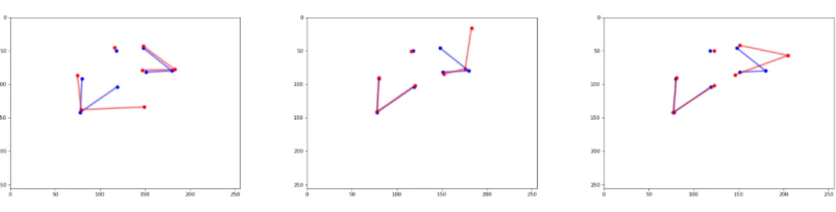
Figure 2.2:PatientPose Soft Failure Anomaly.The visualization of soft failure anomaly can be seen in figure above. The blue is the ground truth pose, the red is the predicted pose. Most soft failure anomaly happens to the wrists, shoulders and elbows. The predicted joint shifts away from the ground truth with a noticeable amplitude.

The soft failure anomaly is defined as the estimated pose still has a human shape, such as small perturbations on couple joints or large perturbations on single joint as indicated in figure 2.2. In other words, non-hard failure anomaly are soft failure anomaly.

(19)

2.2 Anomaly Distribution

2.2.1 Anomaly Joints Distribution

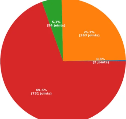
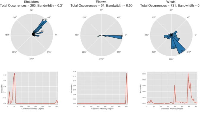
Figure 2.3:Anomaly Joints Distribution.

As in the original paper of PatientPose dataset [1], the smallest joint, wrist, has a width of around 15 pixels in our recordings, we define human error in labeling as up to 15 pixels of euclidean distance between the manually labeled joints and the predicted joints. Hence any joints estimates with an error on or above 15 pixels can be taken as a failure case or anomaly.

(20)

anomalies for different joints can be seen in figure 2.3. Most anomalies occur for the wrists, with a total of 731 wrists out of 3000 frames as anomalies, which makes up over half of all anomalies. The second anomalous joints are the shoulders, with a total of 263 joints as anomaly, a quarter of the all anomalies. The elbows make up a smaller portion of the total anomalies in the dataset. Since there are only two anomalous nose (head) predictions, we dropped nose (head) for the overall PatientPose anomaly analysis.

2.2.2 Anomaly Frames Distribution

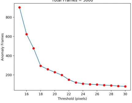
Figure 2.4:PatientPose anomaly frames number across different thresholds.

For anomaly frames distribution, if any joint in the current frame is detected as an anomaly we will take the whole frame as an anomaly detection.

By thresholding the euclidean distance between the manually labeled joints and the predicted joints, we can generate the anomaly pose distribution under different thresholds as indicated in figure 2.4 and table 2.1 with details.

(21)

From figure 2.4, when we increase the threshold from 15 pixel to 18 pixel, increasing the threshold will greatly decrease the anomaly pose number. When we continue increase the threshold from 18 to 23, the anomaly pose number is still going down with a significant slope. After 25 pixels as a threshold, the anomaly pose number started to drop down slowly with a near flat curve.

2.3 Anomaly Modeling

2.3.1 Motivations

We will use a model of anomalies generated from the PatientPose dataset analysis described to generate new anomaly poses from ground truth data. The motivations for anomaly pose modelings: 1. Controllable study of anomaly detection on different joints. 2. Sample infinite anomaly data from the anomaly distribution of the PatientPose framework estimates of poses. 3. Apply sampled anomaly data to our newly annotated 3D dataset of patient poses as testing anomaly data to evaluate our proposed anomaly detection framework performance.

2.3.2 Approach

We model the amplitude, angle and temporal continuity (or “consecutiveness” of the detected anomalies for each joint of interest as indicated in figure 2.5.

(22)

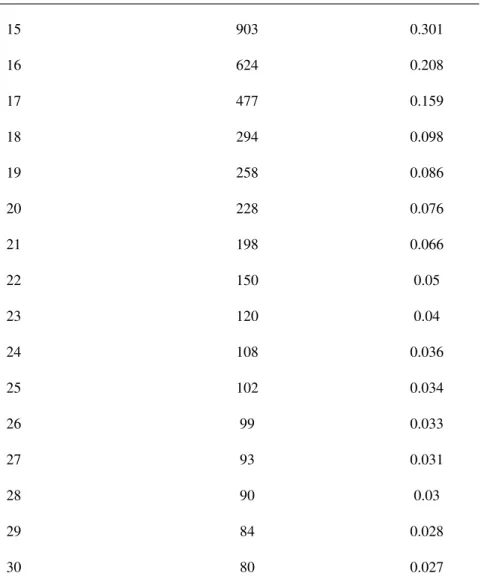
Table 2.1:PatientPose anomaly rate and frames number across different thresholds for anomaly analysis.

Threshold (Pixel) Anomaly Frames (Out of 3000 Frames) Anomaly Rate

15 903 0.301 16 624 0.208 17 477 0.159 18 294 0.098 19 258 0.086 20 228 0.076 21 198 0.066 22 150 0.05 23 120 0.04 24 108 0.036 25 102 0.034 26 99 0.033 27 93 0.031 28 90 0.03 29 84 0.028 30 80 0.027

(23)

Amplitude is defined by the euclidean distance between the estimates joint position and the ground truth in units of pixels.

Angle is defined by setting the origin as the ground truth and the clockwise angle formed from positive Y axis to the segment of anomaly detection and ground truth.

Consecutiveness is defined as the number of sequential frames are anomaly for each joints. By observation of consecutive anomaly frames, the sequential anomaly frames have similar anomaly amplitude and angle.

2.3.3 Method

Kernel Density Estimation

We used Kernel Density Estimation (KDE) to model the distribution of the amplitude, angle and consecutiveness of the anomaly detections for each interested joints as indicated in equations

b pn(x) = 1 nh n

∑

i=1 K(Xi−x h ) (2.1) K(x) = √1 2π e−x 2 2 (2.2)

K(x)is kernel function, in our case is Gaussian. his bandwidth to indicate the smoothness of the PDF curve we are going to get.X iis the data point.nis the number of the data point.

By using KDE, we can sample infinite anomaly data with regarding to the amplitude, angle and consecutive frames number from the real anomaly data we have.

Hyper-parameter tuning

The only hyper-parameter is the bandwidth. To get the optimal bandwidth, we hold an assumption that at least 50 or more data points can generalize the anomaly data distribution. Less than 50 data points

(24)

may not able to generalize the anomaly data distribution. Hence, we drop the head (nose) for the overall PatientPose anomaly detection process. 20 fold cross-validation was applied to perform the hyper-parameter search on bandwidth.

2.3.4 Result

Amplitude

Figure 2.6:Anomaly Amplitude Modeling.

The result of anomaly amplitude KDE modeling can be seen in figure 2.6. The wrists has the largest spectrum in terms of the aanomaly amplitude range from 15 pixel to 50 pixels.

Angle

The result of anomaly angle KDE modeling can be seen in figure 2.7. Anomaly angles are heavily distributed between 45 and 270 clockwise degrees.

Consecutiveness

The result of anomaly consecutiveness modeling can be seen in figure 2.8. We did not applied KDE for consecutiveness distribution. From our observations, a common exponential distribution function can generalize the the distribution very well.

(25)

Figure 2.7:Anomaly Angle Modeling.

Now we can sample anomaly for each joints by sampling from those anomaly models. We can generate equal number of anomaly data for each joints to compare how our framework performs among different joints.

(26)

(27)

Chapter 3 Datasets and Overall System

3.1 Dataset Description

3.1.1 Patient Pose 3D Dataset

In our study, we annotated and conducted our research on recordings of three patients with in-tractable epilepsy. Patients were enrolled according to protocols approved by the Institutional Review Board (IRB) at the New York University (NYU) Langone Comprehensive Epilepsy Center and the Rady Childrens Hospital (RCH), San Diego, Pediatric Epilepsy Center. The video was recorded using a Microsoft Kinect v2 during each patient’s most active period of time. The annotations can be seen in table 3.1. In total, we annotated We 22.4 mins of pose data at 30 fps.

Table 3.1:New dataset annotation details.

Subject Epochs Duration (sec) Frames

S1 61 441.3 13239

S2 51 505.0 15419

(28)

To get the most diverse movements trials from each subject, we used the Gunnar-Farneb¨ack dense optical flow algorithm [12] onto the raw depth video recording of each selected patient to filter out the epochs with movements for each subjects. Under this method, over 50 epochs, each epoch lasts around 10 seconds at 30 FPS, for each subject were selected across the entire recording of each subject’s dataset.

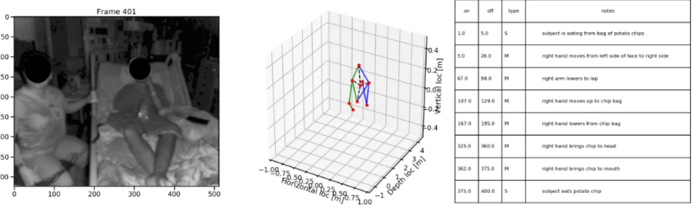
To get the most information of this dataset and empower any follow up clinical patient behavior research, the 3D pose and the movement segments label and description are labeled for each frame. The an-notation for a sample patient can be seen in figure3.1. To ensure the high quality anan-notation, the anan-notation process is peer reviewed by researchers at TNEL.

Figure 3.1:New Dataset Sample.The depth image (left), the 3D pose annotated for current frame (mid), the epoch segments description (right).

It takes dedicated one month to annotate this novel dataset. Based on our segments label, the moving, stable frames number can be seen in table 3.2

To get a high quality dataset for our study. We balance the frames of moving, stable and unified the number of frames for each patient. Frames with significant patient occlusions were excluded. Then we performed camera angle normalization to front camera angle for each patient and train, validation, test spliting by 6:2:2. The detailed dataset used for our study can be seen in table 3.3 for each subject.

Then the test set for each patient was divided by 7:3 for normal poses sequence and anomaly poses sequence. The anomaly poses sequence is created by mapping the anomaly distribution we created from

(29)

Table 3.2:New dataset moving, stable frame number.

Subject Stable Moving Total

S1 8127 5112 13239

S2 9421 5728 15149

S3 5230 6731 11961

Table 3.3:New dataset train, validation, test set.

Subject Training Validation Testing

S1 6000 2000 2000

S2 6000 2000 2000

chapter 2 to each joints. Hence there are different testing set for different interested joints. The testing set divided detail can be seen in table 3.4

In this study we primary focus on upper body pose anomaly analysis and detection. Our interested joints are shoulders, elbows and wrists as we have discusses before.

3.1.2 COCO keypoint dataset

We used COCO keypoint dataset [13] to perform pose modeling. The COCO keypoint dataset [13] was initially proposed to conduct 2D pose detection frameworks. The dataset is made up with train, validation, and test sets, containing more than 200,000 images and 250,000 various scales person instances labeled with keypoints. The 17 keypoints are nose, neck, right-shoulder, right-elbow, right-wrist, left-shoulder, left-elbow, left-wrist, right-hip, right-knee, right-ankle, left-hip, left-knee, left-ankle, left-eye,

(30)

Table 3.4:New dataset testing Set Normal, Anomaly Split

Subject Normal Anomaly

S1 1400 600

S2 1400 600

S3 1400 600

right-eye, left-ear, right-ear. There could be multiple persons in the same image and not all joints are necessary fully labeled. The definition of upper body joints are similar to our PatientPose 3D dataset. It has over 150,000 people and 1.7 million labeled keypoints in total. We do notice some joints are labeled in a poor quality, such as occlusion joints, unseen joints or simply false labels. The COCO dataset annotations were labeled via crowdsourcing Amazon Mechanical Turk. On average, the Amazon Mechanical Turk have a lower precision compare with expert in labeling [13]. Despite the human error in annotations, we assume COCO annotations are ground truth.

3.1.3 Humaneva I dataset

We used Humaneva I dataset [14] to further valid the versatility of our clinical anomaly pose detec-tion system. The Humaneva I dataset [14] is originally proposed to construct and evaluate 3D human pose tracking system. It is professional motion capture system based dataset. It contains 4 gray scale and 3 color calibrated video sequences. The video sequences are synchronized with 3D body poses. There are in total 4 subjects performing common actions. The dataset contains training, validation and testing sets by default. There are 3 angles data from front, left and right of each subject, but we do notice, the data distribution is not even across 4 subjects. And not all of the 4 subjects have decent amount of front angle camera poses. The keypoints are defined in similar fashion as COCO keypoints dataset and PatientPose 3D dataset, but there are also some subtle difference, for instance, the Humaneva define head keypoint as the top of the

(31)

head, where COCO keypoint dataset define it as the nose of the head. In addition, unlike the PatientPose 3D dataset, the Humaneva I dataset is under a lab context with fierce full body movements, where PatientPose 3D dataset is under a clinical context with limited movements freedom given the patients are mostly lying in the bed.

3.2 Overall System

3.2.1 Overall Work Flow

Figure 3.2:Overall work flow.

The figure 3.2 is the overall system flow chart. We first annotated a large scale Patient Pose 3D Dataset. Then we performed data selection for our project to make sure the fairness among different sub-jects. Then we analyzed the PatientPose framework anomaly estimates from previous study. In addition, we performed anomaly modeling for different interested joints based on various factors to achieve

(32)

control-lable/comparable study for each interested joints/subjects. We sampled from the anomaly sampling model to our selected patient pose 3D dataset to form the anomaly detection dataset. Long sequences of poses can have fairly high dimensions, we trained a VAE based model to perform general single pose dimension reduction, as well as single pose anomaly correction. Base on the dimension reduced technic we introduced, we trained models for sequential poses anomaly detection for each subject.

3.2.2 Core Anomaly Detection System

Motivated by the anomaly distribution in chapter 2. The overall deep learning system is constructed with two sub systems. The first stage is the VAE based general pose modeling system for analyzing non-specific poses and give necessary infrastructure for the second stage system. The first stage system can also be used to correct anomaly on joints like shoulder. The second stage is the VAE based subject-specific pose modeling system for analyzing and detecting time sequential anomaly poses. The second stage system is helpful in capture the anomaly joints with movements in a time sequence.

Single Pose Modeling System

Figure 3.3: First Stage Analysis. The input of first stage analysis is the 7 upper body 2D joints with x, y of each joint, in total 14 dimension data. The perfect out put of the first stage VAE decoder should be the same as the normalized input.

For the first stage, we used an variational autoencoder (VAE) [2] based DNN (deep-learning neural networks) to model a general upper body human pose. Hence, when you input an single frame of upper body joints, it will perform location and scale normalization, and then feed into our first stage VAE to reconstruct

(33)

the upper body joints. Based on the similarity of the reconstructed upper body joints and the original input, we can assess if the input joint is anomaly or not. The first stage system can be seen in figure 3.3.

Sequential Poses Modeling System

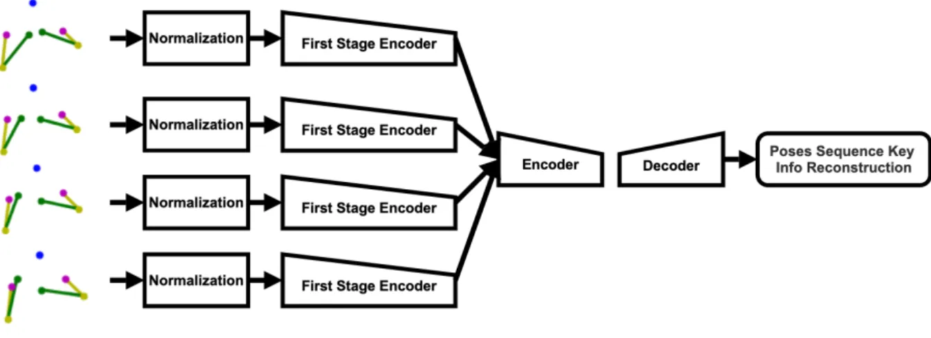
Figure 3.4: Second Stage Analysis.The input of the second stage analysis is a sequence of the subject wise poses, it can be any number of consecutive frames (in the figure above is just an example of consecutive 4 frames)

For the second stage, we used another variational autoencoder (VAE) [2] based DNN (deep-learning neural networks) to model a subject specific upper body human pose continuous sequences. For the input of the second stage VAE, we use the same normalization technique and encoder from the first stage VAE to perform dimension reduction and key information subtraction of each of our subjects continuous pose data. Then we sample the subtracted continues poses into small pose continuous sequences, each sequence is a input unit to the second stage VAE. Hence, we can assess if the input sequence is anomaly or not based on the similarity of the reconstructed sequence and the input sequence. The second stage system can be seen in figure 3.4.

(34)

Chapter 4 Single Pose Modeling

We performed dataset construction, pose normalization, general pose VAE training, general pose modeling analysis in this chapter.

4.1 Dataset Construction

4.1.1 Filtering

For the single pose modeling and anomaly analysis, we used COCO keypoitns dataset. As we men-tioned before, the COCO keypoints dataset is not a perfect dataset. There are in total 273,469 poses in the dataset, only 39,714 poses satisfy our requirements for training first stage VAE. The detailed requirements

Table 4.1:COCO keypoints dataset filtering requirements and corresponding remaining poses.

Requirements Remaining Poses

valid pose 273,469

interested upper body joints fully labeled 100,910 labeled joints should be visible 89,289 joints data should be in valid range 39,714

(35)

Table 4.2:General single poses train, validation, test set.

Training Validation Testing Total

Number of poses 47,656 15,886 15,886 79,428

and filtering process can be seen in table 4.1.

4.1.2 Argumentation

Figure 4.1:General Pose Modeling Data Argumentation.

To train a symmetric pose invariant VAE, after filtering, we performed symmetric data augmentation as indicated in figure 4.1, since the symmetric pose data are also valid. Hence we doubled our valid dataset from 39,741 poses to79,428poses.

4.1.3 Train, Validation, Test Split

(36)

4.1.4 Create Anomaly Data

4.1.5 Argumentation

Figure 4.2:Create Anomaly Data.Here is a visualization of creating anomaly data by perturbing right elbow. The radius of the red circle represents different amplitude of perturbation and the circle represents the random angle.

To validate our single pose modeling framework and pick the best framework for the anomaly correction and anomaly detection. We need perform controllable/comparable anomaly analysis on various upper body joints, hence, we introduced a Euler distance thresholding method to create anomaly data. For the testing set, perturb 1 of the 7 interested upper body joints by radius range from 1 to 100 pixels based on 256 * 256 scale. and random angles. The visualization can be seen in figure 4.2.

4.2 Pose Normalization

In COCO dataset, poses can be in anywhere in the image with any scales. We need train models: 1. Location Invariant 2. Scale Invariant. Hence, we need normalization.

(37)

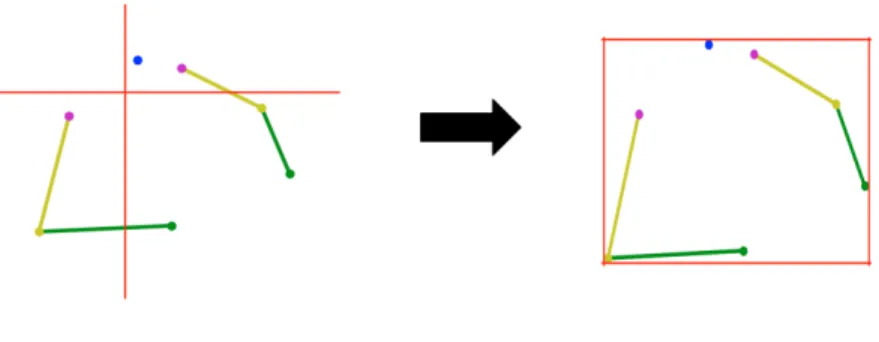
Figure 4.3:General Pose Modeling Pose Normalization.Location normalization left, scale normalization right.

4.2.1 Argumentation

4.2.2 Location Normalization

The poses in COCO keypoints dataset have different locations. In order to achieve location invariant training, we normalized the location (the x, y axis of the upper body joints) of the poses in the dataset we constructed before training. We set the axis origin of each pose as the mid point of the left-shoulder and right shoulder as indicated in the figure 4.3.

4.2.3 Scale Normalization

The poses in COCO keypoints dataset have various scales. In order to achieve scale invariant training, we normalized the scale (the overall size of upper body joints) of the poses in the dataset we constructed before training. We normalized all the poses into 1 by 1 scale as indicated in figure 4.3

(38)

4.3 Training

4.3.1 Loss

The loss function is the sum of the reconstruction loss (Mean Square Error) and the KL Divergence Loss weighted byβ. The detailed loss function can be seen in equations below.

Lossrecon= 1

N N

∑

n=1

(x_iinput−xtout put) (4.1) LossKL=KL(q(z|x)||p(z)), (4.2)

Loss=Lossrecon+β∗LossKL (4.3)

The reconstruction loss measure the difference of the input poses and the reconstructed poses. Hence, if the reconstructed poses are far away the input poses, the reconstruction loss will be high, vice versa. The KL loss will be high if the VAE generated distributionq(z|x)is far away from the real input data distribution p(z)in the latent space, which we assume it to be a normal distribution.

4.3.2 Hyper-parameters

We designed a set of VAEs with single intermediate dense layer in both encoder and decoder. Hence, the remaining hyper-parameters are theβ of KL loss, the intermediate dense layer dimensions and

the latent dimension. The visualization of one of the models can be seen in figure 4.4.

Among all those hyper-parameters, we are most interested in the anomaly detection ability among various latent dimensions of the VAE. Since the latent dimension will determine how many latent dimension is needed to keep all the information we need to reconstruct the pose.

(39)

Figure 4.4:General Single Pose Modeling VAE Example. Here is a visualization of the general pose mod-eling VAE with: 1. Intermediate dense layer dimension: 8. 2. Latent dimension: 2

4.3.3 Architecture

The VAE architecture can be seen in figure 4.5. The input of the the VAE is normalized poses, the output is the reconstructed poses. The encoder will generate the latent variables, the mean and standard deviation vectors of a standard multi-variant Gaussian function. Then we sample from this distribution to feed them into the decoder to generate reconstructed poses.

4.3.4 Result

After training, we picked 7 best models corresponding to 7 different latent dimensions as shown in figure 4.6. From the validation loss history, there are significant loss drop from 2 latent dimension to 10 latent dimension, but there are less difference between 10 to 14 dimension. This can be caused by if the

(40)

Figure 4.5: General Single Pose Modeling VAE Architecture. The output of the encoder is a mean vector and standard deviation vector, which represents the latent space, a multivariate normal distribution. The size of each vector is the latent dimension. We can get the latent vector by sample from the latent space distribution. The sampling process added some variations to the result.

latent dimension is too low, it won’t be able to have all information needed to reconstruct the pose. If the dimension is too high, we already have all the information needed to reconstruct the pose, so keep increasing the latent dimension won’t make any significant difference. Hence we have a hypothesis, the VAE latent dimension have to be at least 10 to get enough information to reconstruct the pose. To validate our hyposis we performed latent space analysis in the following sections.

4.4 Single Pose Modeling Analysis

4.4.1 Latent Space Analysis

One way to analysis if VAE is capable to reconstruct the general pose well is to analysis if it can separate the normal poses from anomaly poses in the latent space. In other words, it is to analysis how the latent space behave when we input poses with different perturbations. For the latent variables, we have mean vector and standard deviation vector. We used t-SNE [15] to visualize the mean vectors distribution in the latent space for training data, testing dataset with 50 pixel perturbations and testing dataset with 100 perturbations for various latent dimensions. The reason behind of only visualize latent mean distribution is the cost-effectiveness. It requires way less computation compare with visualize the whole latent space with

(41)

Figure 4.6:General Single Pose Modeling VAE Training Result.Each line represents the validation loss of the VAE range from 0 to 300 epochs. The different hyper-parameter for each latent dimension is documented in the upper-right legend. The latent is the latent dimension size, the intermediate is the intermediate dimension size, the beta is the KL loss weight index as we discussed before.

the latent standard deviation vector.

As shown in figure 4.7. When we increase the latent dimension to 10, we finally be able to see the separation of all three classes, keep increasing the latent dimension has little effect. Which validated our hypothesis. At least 10 latent dimension is needed to separate anomaly pose and normal pose well. Hence we picked 10 latent dimension model for the first stage pose modeling VAE for the overall system.

4.4.2 Anomaly Correction Analysis

There are some works indicate VAEs are able to generate unseen data, for instance, generating image captions [16] or removing noise in a picture [17], but to our best knowledge, there are no such previous work indicate that VAE is able to correct anomaly poses. We investigate on this intriguing topic

(42)

Figure 4.7:Single Pose Anomaly Analysis t-SNE.t-SNE visualization of latent mean distribution for various latent dimensions. From left to right, first row: latent dimension 2, 4, 6; second row: latent dimension 8, 10, 12; third row: 14.

shown in figure 4.8.

We can first look at head with various latent dimensions.

2 latent dimensions: 2 latent dimension carry too less information about the head location, it studied a relevant fix location of where the head is. 2 latent dimension is able to correct the anomaly after 30 pixel perturbation.

4 latent dimensions: 4 latent dimension still carry not enough data tend to behave like 2 latent dimension. 4 latent dimension model is able to correct the anomaly after 25 pixel perturbation.

(43)

Figure 4.8: Single Pose Anomaly Analysis Anomaly Correction. The X axis is the introduced anomaly perturbation. The Y axis is reconstructed pose compare with unperturbed original pose. The red baseline line is the anomaly created by the perturbation without any correction or inflation by the reconstruction process. If the line is under the baseline, the model have the anomaly correction ability. If the line is on or above the baseline, the model has no anomaly correction ability.

6 latent dimensions: 6 latent dimension will have more information. 6 latent dimension model has less anomaly correction ability for high perturbation.

Higher latent dimensions: Higher dimension data indicate higher reconstruction error. They are generally not good at anomaly correction.

As for other joints. Elbow has a similar behavior as head. All latent dimension models performs well on shoulders anomaly correction. Two shoulders relative locations are easy to learn. Perturb one of the shoulder, its possible to recover it based on the other shoulders location within the upper body. By contrast,

(44)

all latent dimensions models have no anomaly correction ability for wrist. Wrist can be any place in the image. Its not easy to capture the pattern of the wrist.

From this study we know: 1. We can use our trained model to correct anomaly. 2. Our model perform best on shoulder, worst on wrist in terms of anomaly corrections.

(45)

Chapter 5 Clinical Patient Pose Anomaly Analysis

We performed anomaly analysis based on the newly annotated dataset introduced in 2, with a clin-ical context. In this chapter, we discussed the anomaly correction on the PaitientPose framework and the anomaly detection on our newly annotated dataset.

5.1 Anomaly Correction

5.1.1 Shoulders Anomaly Correction

From figure 2.3, we know there are a significant anomaly estimates comes from the shoulders. Based on our previous study in general pose modeling 4.8, we have the model to correct the anomaly shoulders.

To investigate if our general pose modeling technique is able to reduce the anomaly shoulders, we feed in the 3000 frames of pose data from chapter 2 into the pose modeling model with 14 latent dimensions, which performs best in terms of shoulder anomaly correction at 15 pixels anomalous amplitude. The performance of the anomaly correction on shoulder can be seen in the table 5.2.

As indicated in the result table 5.1, there is a substantial anomaly shoulders drop at 15 pixel rules, we reduced about 7.5 % of anomalous shoulders in our dataset.

(46)

Table 5.1: PatientPose anomoly correction on shoulder The anomaly rate is calculated by dividing all anomaly shoulders to all shoulders in our dataset.

Anomaly Shoulders Shoulders Anomaly Rate

Before Anomaly Correction 263 0.043

After Anomaly Correction 240 0.040

Table 5.2: PatientPose enhancementThe shoulders estimation accuracy rate is calculated by average of between the left and right shoulders.

Methods Shoulders Accuracy

PatientPose 95.7

PatientPose + Ours 96.0

5.1.2 PatientPose Enhancement

If we add our anomaly correction as an extra layer to the end of the original PatientPose system, we can improve the shoulders estimation accuracy rate at 15 pixels by about 0.3 %. The similar strategy can be applied to any other upper body pose estimator with similar setting as PatientPose.

5.2 Anomaly Detection

5.2.1 Dataset

As discussed in previous sections, we used the newly annoatated dataset introduced in chapter 3 to conduct the anomaly detection study.

5.2.2 Construct Sequences

The data we have are still sequential poses rather than pose sequences. To investigate the anomaly on pose sequences we have to create corresponding data. For all data, we created sequences of frames range from 2 to 30 as a sequence data by slicing the pose sequence data we have as indicated in figure 5.1.

(47)

Figure 5.1:Subject-specific pose sequence slicing

5.3 Training

5.3.1 Loss

The loss function is the same loss function we used in general pose modeling.

Lossrecon= 1

N N

∑

n=1

(x_iinput−xtout put) (5.1) LossKL=KL(q(z|x)||p(z)), (5.2)

Loss=Lossrecon+β∗LossKL (5.3)

The reconstruction loss measure the difference of the input poses and the reconstructed poses. Hence, if the reconstructed poses are far away the input poses, the reconstruction loss will be high, vice versa. The KL loss will be high if the VAE generated distributionq(z|x)is far away from the real input data distribution p(z)in the latent space, which we assume it to be a normal distribution.

(48)

5.3.2 Hyper-parameters

Similar to the general pose modeling hyper-parameters, we designed a set of VAEs with single intermediate dense layer in both encoder and decoder. Hence, the remaining hyper-parameters to be gird-searched are theβ of KL loss, the intermediate dense layer dimensions, the latent dimension and the number

of consecutive frames in a input data unit.

5.3.3 Architecture

Figure 5.2:Subject-specific Analysis VAE Architecture.Similar as the general pose modeling architecture. The output of the encoder is a mean vector and standard deviation vector, which represents the latent space, a multivariate normal distribution. The size of each vector is the latent dimension. We can get the latent vector by sampling from the latent space distribution. .

From our previous study on general pose modeling, we used 10 latent dimension pose modeling model to perform dimension reduction on our newly annotated dataset.

The VAE architecture can be seen in figure 5.2. The VAE architecture is similar to the VAE archi-tecture for general pose modeling. But the input and output are different, the input of the the VAE is pose sequence key information, the output is the reconstructed pose sequence key information. The encoder will generate the latent variables, the mean and standard deviation vectors of a standard multi-variant Gaussian function. Then we sample from this distribution to feed them into the decoder to generate reconstructed pose sequence key information.

(49)

Table 5.3:Subject-specific Training Result S1.Best model for various consecutive frames.

Consecutive Frames Latent Dimension Intermediate Dimension KL Index

2 12 20 0.0001 4 32 40 0.0001 6 24 60 0.0001 8 48 80 0.0001 10 100 100 0.0001 12 72 120 0.0001 14 56 140 0.0001 16 64 160 0.0001 18 144 180 0.0001 20 160 200 0.0001 22 132 220 0.0001 24 96 240 0.0001 26 104 208 0.0001 28 112 280 0.0001 30 120 300 0.0001

(50)

2 20 20 0.0001 4 32 40 0.0001 6 36 60 0.0001 8 32 80 0.0001 10 80 100 0.0001 12 48 96 0.0001 14 56 140 0.0001 16 96 160 0.0001 18 72 180 0.0001 20 80 200 0.0001 22 88 220 0.0001 24 96 240 0.0001 26 104 260 0.0001 28 112 280 0.0001 30 120 300 0.0001

(51)

2 12 20 0.00001 4 40 40 0.00001 6 48 60 0.00001 8 32 80 0.00001 10 60 100 0.00001 12 120 120 0.00001 14 140 140 0.00001 16 160 160 0.00001 18 108 180 0.00001 20 120 200 0.00001 22 88 220 0.00001 24 96 240 0.00001 26 104 260 0.00001 28 112 280 0.00001 30 180 300 0.00001

(52)

5.3.4 Result

After training, we picked best models corresponding to 15 different consecutive frames as a single data sequence for subject 1, subject 2 and subject 3. The details can be see in figure 5.3, 5.4 and 5.5.

5.4 Anomaly Analysis

5.4.1 Consecutive Frames as A Sequence

We use Area Under Curve (AUC) to measure the performance cross different number of frames as a sequence data. Since we want high level comparison among different consecutive frames models to find the best model for each subject.

The best (highest AUC) consecutive frames number as a sequence anomaly detector model among different subjects various based on the different movement speed and pattern for different subjects, for subject 1 is 14, subject 2 is 8, for subject 3 is 4.

5.4.2 Comparison

Figure 5.3:Anomaly Detection RoC Curves for Subject 1.

(53)

figures 5.3, 5.4 and 5.5. For the trade off between TPR and FPR. If we have less tolerance to normal pose being detected as anomaly, low FPR is desired. If we have less tolerance to anomaly poses are not detected, high FPR is desired. We also compare our VAE based method to other two methods OC-SVM and Isolation Forest with the same input and output with the best model from hyper-parameter search.

In general, our method performs the best among all those three methods in terms of AUC. This can be caused by the deep learning based framework can study more details about our sequential pose data compare with traditional machine learning based anomaly detection methods.

For subject 1, our method greatly out performed the other two methods for all joints. More detailed AUC for each method can be seen in table 5.6.

(54)

Table 5.6:Anomaly Detection AUC Comparison.Compare the AUC under various methods for each subject.

Subject 1

Method Shoulders Elbows Wrist Isolation Forest 0.67 0.45 0.44

OC-SVM 0.34 0.32 0.28

Ours 0.95 0.74 0.77

Subject 2

OC-SVM 0.59 0.6 0.52

Ours 0.83 0.80 0.75

Subject 3

OC-SVM 0.71 0.68 0.66

Ours 0.88 0.81 0.80

For subject 2 and subject 3, for the shoulder, our methods under performs IsolationForest in terms of TPR under a relative small FPR. This can be caused by, in the clinical environment, the patient is lying in the bed during the most time. And the action performed by the patient in the bed are usually not involved with shoulder movements. So shoulder have a minimal freedom of movements in the clinical environment. In addition, IsolationForest is a simple anomaly detection method, that measure the difficulty to isolate a data point from the rest data, which is supposed to work well on the data point with relative high consis-tency. However, this does not apply to subject 1 which our method still out performs the rest methods. By inspecting the recording of subject 1, there are more complex movements for subject 1, such as playing toy bear, eating food on the table, interacting with other people in the room, but there are less complex move-ments performed by subject 2 and 3. For the most simple anomaly data, the Isolation Forest may performs better than deep learning based method.

(55)

In this case we can greatly reduce the manual labor. For instance, if we use our method for the shoulder anomaly for S3, we have a TPR as 1.0 when the False Positive Rate (FPR) is only around 0.2. Based on the percentage of the anomaly data we have, we can save up to 80 % manual labor to find those anomaly data.

(56)

Chapter 6 Framework Versatility Analysis.

In this chapter we performed anomaly detection on a general public sequential human pose dataset Humaneva [14] for subject-specific pose anomaly analysis to test our frameworks’s performance on non-clinical based environment.

6.1 Dataset Construction

6.1.1 Train, Validation, Test Split

Humaneva dataset [14] for subject-specific pose anomaly analysis. It was originally proposed to research on 3D human pose tracking system. It is professional motion capture system based with high accurancy. The dataset contains 4 subjects. 4 grayscale and 3 color calibrated video sequences at 60 fps. There are 3 angles data from front, left and right of each subject. We finalized 2 valid subjects to perform

Table 6.1:Subject-specific poses train, validation, test set.

S1 754 251 251

(57)

Table 6.2:Subject-specific poses train, validation, test set with argumentation

S1 2262 251 251

S2 2310 256 256

Table 6.3:Subject-specific testing Set Normal, Anomaly Split

Subject Normal Anomaly

S1 175 76

S2 179 79

the task. We used valid front-camera angle data from Humaneva dataset. Datasets Splitting: 6 : 2 : 2 for training, validation and testing, can be seen in table 6.1.

6.1.2 Argumentation

We performed training data argumentation by rotating the pose by Z axis, clockwise 10 degree and counter-clockwise 10 degree, and then project new 3D pose to front-camera angle. Hence we tripled out training dataset. The augmented dataset can be seen in table 6.2.

6.1.3 Testing Set Normal, Anomaly Split

To test on our testing dataset, we have to have anomaly data in our testing set. We split the testing set into normal data: anomaly data by 7: 3 as indicated in table 6.3.

(58)

6.1.4 Construct Sequences

The data we have are still sequential poses rather than pose sequences. To investigate the anomaly on pose sequences we have to create corresponding data. For all data, we created sequences of frames range from 2 to 30 as a sequence data by slicing the pose sequence data we have as indicated in figure 5.1.

6.1.5 Create Anomaly Data

We have already have the anomaly data splitting in the testing dataset, but all those data are normal data. We need added perturbation to those data to create anomaly. We performed adding anomaly data by adding perturbation from 1 to 100 pixels radius, with random angle (as we did in general pose anomaly analysis ) to a random pose in a unit pose sequence for each of seven upper body joints.

6.2 Training Result

The training loss, hyper-parameters and architecture are the same as the previous chapter.

After training, we picked best models corresponding to 15 different consecutive frames as a single data sequence for subject 1 and subject 2 as shown in figure 6.4 and 6.5.

6.3 Anomaly Analysis

6.3.1 Various Consecutive Frames as A Sequence

We use Area Under Curve (AUC) to measure the performance cross different number of frames as a sequence data. Since we want high level comparison among different consecutive frames models. We mainly focus on AUC at 60 pixel perturbations. As we discussed before there is human error involved in labeling process. We can define human label error about 15 pixels with the similar concept introduced in PatientPose [1], which is around 3 inches. 60 pixel is 9 inches away from human error, which we can truly

(59)

Table 6.4:Subject-specific Training Result.Best model for various consecutive frames.

2 8 20 0.0001 4 16 40 0.0001 6 24 60 0.0001 8 32 80 0.0001 10 40 100 0.0001 12 48 120 0.0001 14 56 140 0.0001 16 64 128 0.0001 18 72 180 0.0001 20 80 200 0.0001 22 88 220 0.0001 24 96 192 0.0001 26 104 208 0.0001 28 112 280 0.0001 30 120 240 0.0001

(60)

Table 6.5:Subject-specific Training Result.Best model for various consecutive frames.

2 8 20 0.0001 4 16 32 0.0001 6 24 48 0.0001 8 32 80 0.0001 10 40 80 0.0001 12 48 120 0.0001 14 56 140 0.0001 16 64 160 0.0001 18 72 144 0.0001 20 80 200 0.0001 22 88 220 0.0001 24 144 192 0.0001 26 104 208 0.0001 28 112 224 0.0001 30 120 240 0.0001

(61)

Figure 6.1:Subject-specific Analysis on Various Consecutive Frames as A Sequence Subject 1.

call it an anomaly. The figure for subject 1 and subject 2 can be seen in figure 6.1 and 6.2.

As for performance among different consecutive frames as a unit data, for both subjects, perfor-mance of 4 consecutive frames as a unit data performs best. 2 consecutive frames as a sequence data may not able to learn the association between poses. Higher frames as a unit data may have less effect for only one random perturbed frame in each unit data.

As for performance among different joints, for both subjects, elbow have a similar trend as what we saw in nose. Shoulder has a different trend when we have a perturbation greater than 60 pixels. This can be

(62)

Figure 6.2:Subject-specific Analysis on Various Consecutive Frames as A Sequence Subject 2.

the anomaly correction ability of shoulder for the pose modeling. Wrist has a different trend compare to all other joints. Which validate our previous study, wrist is hard to be modeled.

As for performance among two subjects. Subject 2 has a great drop from subject 1 in terms of AUC. After we For subject 2. Many frames have only one-side body exposed. Unseen upper body joints not satisfy our general modeling VAE input data requirements.

(63)

Figure 6.3:4 Consecutive Frames as A Sequence Subject 1 at 60 pixel perturbations.

6.3.2 Comparison

RoC curve for nose at 60 pixel perturbation for 2 subjects with true positive rate (TPR) and false positive rate (FPR) can be seen in figures 6.3 and 6.4. We compare our VAE based method to other two methods OC-SVM and Isolation Forest with the same input and output with the best model from hyper-parameter search.

For the trade off between TPR and FPR. If we have less tolerance to normal pose being detected as anomaly, low FPR is desired. If we have less tolerance to anomaly poses are not detected, high FPR

(64)

Figure 6.4:4 Consecutive Frames as A Sequence Subject 2 at 60 pixel perturbations.

is desired. For subject 1, we may chose OC-SVM for low FPR or our VAE based method for high TPR, Isolation Forest is no good in either cases.

For the performance among different methods. Our VAE method performs best in terms of AUC. As we can see in table 6.6. As we discussed before the result for subject 2 has a drop form subject 1 due to the failure data-set.

Even we can’t directly compare with the result of the HumanEva dataset to our PatientPose 3D dataset. The performance on HumanEva dataset is not as good as Patient Pose 3D dataset. This can be

(65)

Table 6.6: 4 Consecutive Frames as A Sequence at 60 pixel perturbations AUC Comparison. Compare the AUC at 60 pixel perturbation of various methods for each subject.

Subject 1

Method Nose Shoulders Elbows Wrist Isolation Forest 0.72 0.65 0.67 0.72

OC-SVM 0.78 0.7 0.73 0.7

Ours 0.8 0.78 0.79 0.75

Subject 2

Method Nose Shoulders Elbows Wrist Isolation Forest 0.66 0.56 0.59 0.59

OC-SVM 0.52 0.46 0.47 0.49

Ours 0.69 0.67 0.68 0.67

caused by several factors. First, we have way more training data for PatientPose 3D dataset compare to HumanEva dataset. Second, we introduced the consecutive anomaly poses testing data in our PatientPose 3D anomaly detection, where as we only tested with single frame anomaly in HumanEva dataset. Third, HumanEva dataset have fierce full body movements (running, throw and catch and boxing) compare with the the PatientPose 3D dataset, where during the most of the time the patient is lying or sitting in the bed.

(66)

Chapter 7 Conclusion and Future Work

In this chapter we summarized main contributions in this study and discussed possible future work.

7.1 Conclusion

We address the issue of lacking high quality, large scale clinical patient pose dataset by constructing a novel 3D patient pose dataset consisting of 3 subjects with around 22.4 mins recording at 30 fps. To ensure the high quality dataset, the quality of the annotation has been reviewed by researchers at TNEL.

Our general pose modeling framework have the ability to correct anomaly pose, it works well on shoulders, which reduced shoulder anomaly rate about 7.5 % on the PatientPose framework.

We developed a method to model real anomaly distributions to study the anomaly detection on each interested joint. Our VAE based clinical subject-specific pose anomaly detection have the best anomaly detection performance compare with general anomaly detectors such as OC-SVM and Isolation Forest in terms of AUC. For certain joints and subject, our method can save around 50% to 80% manual labor to identify anomalous estimates.

(67)

7.2 Future Work

Since the subjects in our study were implanted with either electrocorticography (ECoG) or stere-oelectroencephalography (sEEG) electrodes for electrophysiological monitoring of epileptic seizures. By aligning the ECoG and sEEG recording to our annotated patient pose dataset, many studies on neurophysi-ology for seizure patients can be done.

We annotated a new 3D clinical patient pose dataset from the depth data. But our current Patient-Pose framework does not support 3D pose estimation in the clinical environment. We can develop a 3D PatientPose framework from our newly labeled dataset.

(68)

References

[1] Kenny Chen, Paolo Gabriel, Abdulwahab Alasfour, Chenghao Gong, Werner K Doyle, Orrin Devin-sky, Daniel Friedman, Patricia Dugan, Lucia Melloni, and Thomas Thesen. Patient-specific pose esti-mation in clinical environments. IEEE Journal of Translational Engineering in Health and Medicine, 6:1–11, 2018.

[2] Diederik P Kingma and Max Welling. Auto-encoding variational bayes. arXiv preprint arXiv:1312.6114, 2013.

[3] Fei Tony Liu, Kai Ming Ting, and Zhi-Hua Zhou. Isolation forest. In2008 Eighth IEEE International Conference on Data Mining, pages 413–422. IEEE, 2008.

[4] Roberto Perdisci, Guofei Gu, and Wenke Lee. Using an ensemble of one-class svm classifiers to harden payload-based anomaly detection systems. InICDM, volume 6, pages 488–498. Citeseer, 2006. [5] Kevan Yuen and Mohan M Trivedi. Looking at hands in autonomous vehicles: A convnet approach

using part affinity fields.IEEE Transactions on Intelligent Vehicles, 2018.

[6] Zhijie Fang and Antonio M L´opez. Is the pedestrian going to cross? answering by 2d pose estimation. In2018 IEEE Intelligent Vehicles Symposium (IV), pages 1271–1276. IEEE, 2018.

[7] Yao-Jen Chang, Shu-Fang Chen, and Jun-Da Huang. A kinect-based system for physical rehabilita-tion: A pilot study for young adults with motor disabilities. Research in developmental disabilities, 32(6):2566–2570, 2011.

[8] Zhengyou Zhang. Microsoft kinect sensor and its effect. IEEE multimedia, 19(2):4–10, 2012. [9] Aouaidjia Kamel, Bin Sheng, Po Yang, Ping Li, Ruimin Shen, and David Dagan Feng. Deep

convo-lutional neural networks for human action recognition using depth maps and postures. IEEE Transac-tions on Systems, Man, and Cybernetics: Systems, (99):1–14, 2018.

[10] Zhenghua Chen, Qingchang Zhu, Yeng Chai Soh, and Le Zhang. Robust human activity recognition using smartphone sensors via ct-pca and online svm. IEEE Transactions on Industrial Informatics, 13(6):3070–3080, 2017.

[11] Yaqiang Yao, Yan Liu, Zhenyu Liu, and Huanhuan Chen. Human activity recognition with posture tendency descriptors on action snippets.IEEE Transactions on Big Data, 4(4):530–541, 2018. [12] Gunnar Farneb¨ack. Two-frame motion estimation based on polynomial expansion. InProceedings of

(69)

[13] Tsung-Yi Lin, Michael Maire, Serge Belongie, James Hays, Pietro Perona, Deva Ramanan, Piotr Doll´ar, and C Lawrence Zitnick. Microsoft coco: Common objects in context. InEuropean conference on computer vision, pages 740–755. Springer, 2014.

[14] Leonid Sigal, Alexandru O Balan, and Michael J Black. Humaneva: Synchronized video and mo-tion capture dataset and baseline algorithm for evaluamo-tion of articulated human momo-tion. International journal of computer vision, 87(1-2):4, 2010.

[15] Laurens van der Maaten and Geoffrey Hinton. Visualizing data using t-sne. Journal of machine learning research, 9(Nov):2579–2605, 2008.

[16] Yunchen Pu, Zhe Gan, Ricardo Henao, Xin Yuan, Chunyuan Li, Andrew Stevens, and Lawrence Carin. Variational autoencoder for deep learning of images, labels and captions. In Advances in neural information processing systems, pages 2352–2360, 2016.

[17] Daniel Im Jiwoong Im, Sungjin Ahn, Roland Memisevic, and Yoshua Bengio. Denoising criterion for variational auto-encoding framework. InThirty-First AAAI Conference on Artificial Intelligence, 2017.