Volatility and growth

V

OLATILITY AND

G

ROWTH

Viktoria Hnatkovska

Norman

Loayza

August 2003

Abstract

This paper studies the empirical, cross-country, relationship between macroeconomic volatility and long-run economic growth. It addresses four central questions. The first is whether the volatility-growth link depends on country and policy characteristics, such as the level of development or trade openness. The second one is whether this link reflects a statistically and economically significant causal effect from volatility to growth. The third question concerns the stability of this relationship over time and whether it has become stronger in recent decades. And the fourth is whether the volatility-growth connection actually reveals the impact of crises rather than the overall effect of cyclical fluctuations. We find that indeed macroeconomic volatility and long-run economic growth are negatively related. This negative link is exacerbated in countries that are poor, institutionally underdeveloped, undergoing intermediate stages of financial development, or unable to conduct countercyclical fiscal policies. We find evidence that this negative relationship actually reflects the harmful effect from volatility to growth. Furthermore, we find that the negative effect of volatility on growth has become considerably larger in the last two decades and that it is mostly due to large recessions rather than normal cyclical fluctuations.

*_{We thank Megumi Kubota for able research assistance in the preparation of the database used in}

the paper. We are grateful to Joshua Aizenman, Luis Servén, Brian Pinto, and specially, Ricardo Caballero for their comments and suggestions. V. Hnatkovska is affiliated to Georgetown University, and N. Loayza, to the World Bank. The usual disclaimer applies.

Public Disclosure Authorized

Public Disclosure Authorized

Public Disclosure Authorized

Public Disclosure Authorized

VOLATILITY AND GROWTH

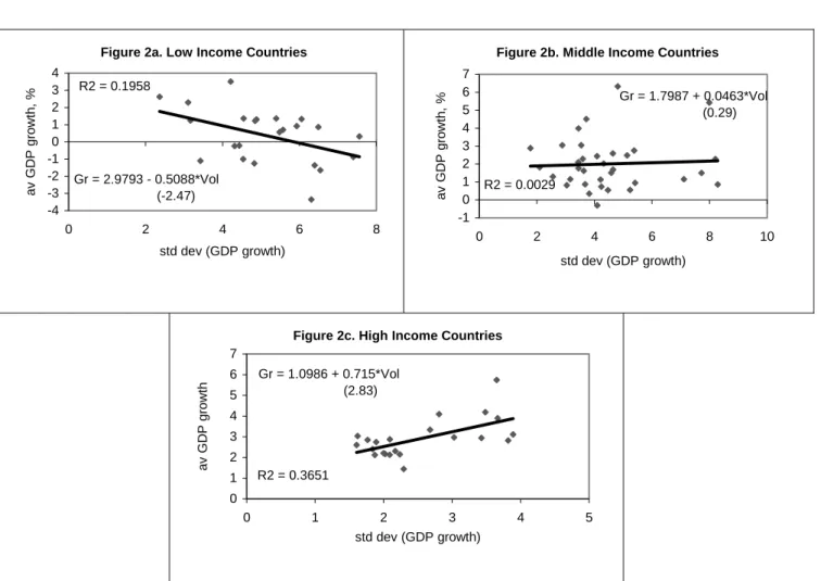
In the last four decades, at least the 40 most volatile countries in the world are developing economies. Among the most volatile, there are not just small economies, such as the Dominican Republic or Togo, but also large countries, such as China and Argentina. Many of them are mainly commodity exporters, like Nigeria and Ecuador, but some are also rapidly industrializing countries, such as Chile and Indonesia. At the other extreme of the spectrum, nine of the ten least volatile countries in the World belong to the OECD. The connection between volatility and lack of development is undeniable, but is volatility also related to economic growth? Judging by simple cross-country correlations, there appears to be a negative relationship between the average and the standard deviation of per capita GDP growth, both calculated over long periods (see Figure 1). However, this connection is not uniform but seems to depend on structural country characteristics. For example, while the correlation between volatility and growth is negative for poor countries, it is basically zero for middle-income countries and even positive for the group of rich economies (see Figure 2).

From academic and policy perspectives, there are four central questions on the relationship between volatility and growth that we address in this paper. The first is whether this link depends on country and policy characteristics, such as the level of development or trade openness. The second one is whether the link reflects a causal effect from volatility to growth and, if so, whether this effect is statistically and economically significant. The third question concerns the stability of this relationship over time, and in particular whether recent decades feature a stronger relationship between volatility and growth. The fourth question is whether the volatility-growth connection actually reveals the negative impact of crises rather than the overall effect of cyclical fluctuations.

With these questions in mind, this study documents the relationship between macroeconomic volatility and long-run economic growth. Its approach is mostly empirical and relies on cross-country comparisons. However, in order to help understand and put into context the empirical results, the first section of the paper selectively reviews the analytical literature on the volatility-growth relationship. The second section

describes the data and econometric methodologies used in the empirical sections of the paper. Of special importance is the discussion on the various measures of volatility and economic crises.

Section III presents new empirical results, following the questions outlined above. Thus, using interaction terms in the regression analysis, we first attempt to determine whether there is a significant link between volatility and growth under various structural country characteristics. These are the country’s overall level of development, the degree of openness to international trade, the extent of financial depth, the level of institutional development, and the degree of fiscal policy procyclicality. Second, using instrumental variables inspired from the causes-of-volatility literature, we account for the likely endogeneity of volatility with respect to economic growth and its determinants. In this way, we try to ascertain the causal effect from macroeconomic volatility to long-run growth. Third, we compare the volatility-growth link for the four decades since the 1960s, paying special attention to the break that researchers have observed before and after the 1980s. We do the decade comparison both ignoring and accounting for the potential endogeneity of macroeconomic volatility. Finally, we analyze whether the negative connection between volatility and growth may be due in fact to the consequences of economic crises. We do it by contrasting the growth effects of repeated but small cyclical fluctuations (“normal volatility”) and large and lasting negative macroeconomic fluctuations (“crises”). Section IV offers selected concluding remarks, together with some practical quantifications of the relationship between macroeconomic volatility and long-run economic growth.

I. ANALYTICAL BACKGROUND.

Traditionally, the literatures on long-run growth and business cycles have remained apart. This approach, however, has been challenged by recent theories and evidence that establish a strong connection between business-cycle behavior and long-run performance (for reviews see Fatás 2002 and Wolf 2003; for theoretical analyses, see Caballero and Hammour 1994, and Aghion and Saint-Paul 1998; and for empirical evidence see Ramey and Ramey 1995, Martin and Rogers 2000, Kroft and Lloyd-Ellis 2002, and Servén 2003). One aspect of this relationship is the link between

macroeconomic volatility and economic growth. In theory, this link could result from the joint determination of volatility and growth as endogenous variables or could stem from a causal effect from one variable to the other. Moreover, the relationship between volatility and growth may be positive or negative depending on the mechanisms driving the relationship (see Imbs 2002).

Let’s consider first the case when both variables are jointly determined. Their link could be positive if volatility and long-run growth reflect the risk and mean return characteristics of investment projects: countries that aim at higher average growth rates must accept correspondingly higher risks. For this argument to hold, however, it would be necessary for countries to have sufficiently well developed financial markets and government institutions, including judicial courts. Without risk-sharing mechanisms and proper monitoring and enforcement of contracts, investors would not pursue risky projects that would be otherwise optimal.

A different approach to analyze the joint determination of volatility and growth derives from considering asymmetric effects of business-cycle fluctuations. On the one hand, a positive link could develop as follows. If volatility is associated with the occurrence of recessions, and if recessions lead to higher research and development and/or the destruction of least productive firms, then higher long-run growth can occur alongside higher volatility. This is the “creative destruction” view that dates back at least to Schumpeter (1939). (For a modern treatment of this view, see Shleifer 1986, Hall 1991, Caballero and Hammour 1994, and Aghion and Saint-Paul 1998). Again, this argument requires deep financial markets, active firm turnover, and the ability to conduct counter-cyclical educational and innovation expenditures, characteristics that are usually associated with developed economies. On the other hand, a negative link between volatility and growth could occur if recessions are tied to a worsening of financial and fiscal constraints, which is more likely to occur in developing countries. In this case, recessions can lead to less human capital development --by decreasing learning-by-doing, for instance--, lower productivity-enhancing expenditures, and, thus, smaller growth rates (see Martin and Rogers 1997, and Talvi and Vegh 2000). Moreover, aversion to economic recessions could prompt governments to adopt policies, such as labor-market

restrictions, that make firms less flexible and willing to innovate, thus deepening a negative link between volatility and long-run growth.

The connection between volatility and growth can also result from a causal relationship. For our purposes, we concentrate on the potential impact of volatility on growth. This effect will be mostly negative when volatility is associated with economic uncertainty, whether this comes from political insecurity (Alesina et al. 1996), macroeconomic instability (Judson and Orphanides 1996), or institutional weaknesses (Servén 2000, and Rodrik 1991). The theoretical underpinnings for a negative effect of uncertainty on economic growth operate through conditions of risk aversion, lumpiness, and irreversibility associated to the investment process: under these conditions, uncertainty is likely to lead firms to under invest or invest in the “wrong” projects (see Bertola and Caballero 1994). Some country structural characteristics are bound to worsen the impact of volatility and uncertainty on economic growth, such as a poor level of financial development, deficient rule of law, and procyclical fiscal policy, which usually accompanies large public indebtedness (see Caballero 2000).

In this study, we are interested in the empirical regularities dealing with both the overall relationship between volatility and growth and the causal effect from the former to the latter. Considering the analytical background just summarized, we will consider both the role of country structural characteristics in shaping this mutual relationship and the role of factors that drive volatility in order to estimate its exogenous impact on growth.

II. METHODOLOGY AND DATA.

We are interested in describing the empirical, cross-country connection between macroeconomic volatility and long-run economic growth. For this purpose, we examine a variety of empirical models where a country’s economic growth is the dependent variable and its volatility, the main explanatory variable. Our statistical units are given by country observations with data representing averages over relatively long periods. The majority of our empirical exercises are conducted using only cross-sectional data, specifically, country-averages over the period 1960-2000. Since we are also interested in testing the stability of the volatility-growth relationship over time, in some cases we work

with country averages by decades, spanning the same period. What follows describes our empirical strategy and data in detail.

A. Empirical Methodology. We follow the main strand of the new growth

literature in the choice of both the dependent and explanatory variables, to which we add two volatility measures (see Barro 1991). We proceed as follows. We start by examining the simple regression of the growth rate of per capita GDP on each of two measures of macroeconomic volatility (defined below). We do it for the full sample of countries and for various country groupings determined by criteria such as the level of overall development, financial depth, trade openness, institutional development, and fiscal policy procyclicality. This simple growth regression is represented by,

i i

i vol

gr =β₀ +β₁ +ε

where gr represents average growth rate of per capita GDP, vol is a volatility measure, ε

is the regression residual, and i is a country index.

Next, we assess the link between volatility and growth after controlling for other variables that affect a country’s growth process. This allows us to examine whether the simple link between volatility and growth is channeled through regular growth determinants. The corresponding growth regression is given by,

gr_i =β₀ +β₁vol_i +β₂X_i +ε_i

where X represents a set of control variables, including the initial level of GDP per capita (to account for transitional convergence effects), the average ratio of domestic private credit to GDP (as proxy for financial development), and the average secondary school enrollment ratio (to account for human capital investment). These control variables are chosen in consideration of their robust role in the new empirical growth literature (see

Levine and Renelt 1992).1

We then conduct an extension of the regression analysis by considering whether the size and statistical significance of the volatility-growth relationship varies according to the structural characteristics mentioned above. We account for these multiplicative effects through both continuous and categorical interactions between volatility and

1

We also considered an expanded set of control variables, including measures of trade openness, government consumption, and institutional development. Although in some cases these variables presented significant coefficients, the volatility-related results discussed in the paper were qualitatively the same.

country structural characteristics in the corresponding growth regressions. The corresponding regression equations are given by,

i i i

i i

i vol vol Struct X

gr =β0 +β1 +β2 * +β3 +ε

where Struct represents, in turn, the following structural country characteristics: overall economic development (proxied by the level of output per capita), financial depth (measured by the ratio of private domestic credit to GDP), international trade openness (proxied by the ratio of real exports plus imports to GDP), the level of institutional development (measured by a subjective index of investor perceptions –the ICRG index), and the degree of fiscal policy procyclicality (proxied by the correlation coefficient between the growth rate of GDP and the growth rate of government consumption as share

to GDP).2

The country characteristics represented in Struct are considered in two ways. The first one is standard and consists of Struct taking the actual values of the corresponding measures for each country. This is the case of a “continuous” interaction with volatility (or simple multiplicative effect). The second way of accounting for structural characteristics is through country groups (or categories) derived from the cross-country ranking for each characteristic; specifically, in each case, we work with three similarly-sized groups of countries --low, medium, and high. Then, the variable Struct acts as a “dummy” variable that indicates whether a country belongs or not to a given group. This is the case of a “categorical” interaction with volatility, and it allows for a non-monotonic relationship between volatility and growth.

Next, attempting to go beyond the description of mutual relationships, we take into account the possibility that volatility may be endogenously determined together with long-run growth. We use an instrumental-variable procedure to isolate exogenous changes in volatility and, thus, gauge their causal impact on per capita GDP growth. The regression model then becomes,

i i i i vol X gr =β₀ +β₁ +β₂ +ε i i i IV u vol =γ1 + 2

We also considered the production structure of the economy, specifically the share of agricultural value added in GDP. However, this structural characteristic did not seem to affect the volatility-growth relationship in a robust or significant manner.

0 ) * ( but 0 ) * (voli i ≠ E IVi i = E ε ε

where IV represents a set of instrumental variables for volatility, whose desired properties are that they help explain volatility but at the same time affect long-run growth only through volatility (and the other control variables). We choose the set of instrumental variables for their importance in the macroeconomic stabilization literature. They are the standard deviation of the inflation rate, a measure of real exchange rate misalignment, the standard deviation of terms of trade shocks, and the frequency of systemic banking crises. These variables highlight the point that macroeconomic volatility can be driven by non-policy factors (e.g., the volatility of terms of trade shocks) or a combination of non-policy and non-policy elements (all the rest).

We then repeat the regression analysis --with and without interaction terms and instrumental variables-- for the database organized as country averages by decades. For the majority of countries, we work with 4 observations each, corresponding to the 1960s, 70s, 80s, and 90s. Our objective is to assess how the volatility-growth connection has changed over time, and in particular, whether it has increased in the 1980s and 90s. For this purpose, we use the pooled cross-section, time-series data to estimate jointly the coefficients on volatility for each decade and then test whether their differences are statistically significant. The pooled regression model is given by,

t i t i t i t t t i vol X gr_, = β_0, +β_{1, ,} +β_{2 ,} +ε_,

where the subscript t denotes time periods (decades). Note that we allow the volatility coefficient to be different across decades. As mentioned above, we extend this regression to account for the joint endogeneity of volatility and its dependence on the level of income.

Finally, we examine whether the negative association between volatility and growth could reflect the harmful impact of sharp negative fluctuations (crisis volatility) rather than the effect of repeated but small cyclical movements (normal volatility). For this purpose, we modify the regression analysis by replacing the (overall) volatility measure by two of its components, that is, one related to “normal volatility” and the other representing “crisis volatility.” The measurement of these volatility components is described in the next section. The growth regression equation then becomes,

i i i i i NormalVol CrisisVol X gr =β0 +β1 +β2 +β3 +ε

where NormalVol and CrisisVol represent the normal and crisis components of volatility, respectively. We estimate this regression both ignoring and accounting for the potential endogeneity of the volatility components. We expand the set of instruments by generating the “crisis” versions of our instruments and adding them to the regular set.

B. Sample and Data. We work with both a single cross-section of countries and

a pooled sample of country and time series observations. In the case of a single cross-section, the observations correspond to country averages for the period 1960-2000. The pooled sample consists of decade averages per country, corresponding to 1961-70, 1971-80, 1981-90, and 1991-2000. The pooled dataset is almost fully balanced in the sense that for close to 95% of the countries we have complete data for each of the four decades. The resulting sample consists of 79 countries, of which 22 are OECD. Regarding developing countries, 21 belong to Latin America and the Caribbean, 19 to Sub-Saharan Africa, 8 to the Middle East and North Africa, 6 to East Asia and the Pacific, and 4 to South Asia.

We measure macroeconomic volatility in two different ways. Both focus on overall output volatility --as a summary proxy for macro volatility--, and both intend to capture the variability of cyclical macroeconomic fluctuations. Following most of the empirical literature on volatility, the first measure is the standard deviation of per capita GDP growth, calculated for each country over the corresponding sample period. The second one follows the real business cycle literature and consists of the standard deviation of the per capita GDP gap. This involves estimating the trend of each country’s per capita GDP series, obtaining the gap between actual and trend GDP, and then calculating the standard deviation of the gap series. We estimate each country’s trend GDP series by applying the band-pass filter developed by Baxter and King (1999) to the country’s GDP series. The first volatility measure implicitly assumes that trend GDP grows at a constant rate, whereas the second measure allows trend GDP to follow a richer, time- and country-dependant process. The standard deviation of GDP growth would exaggerate macro volatility if actual GDP growth has an upward or downward trend (which is the case for economies in transition to their long-run steady state). On the other hand, the standard deviation of the output gap may underestimate macro volatility if

the trend series follows the actual one too closely. In practice, however, the two volatility measures are highly correlated in the cross-country dimension and render quite similar results in this paper. The coefficient of correlation between the two volatility measures is 0.98 for the full sample and above 0.89 for any of our country groups.

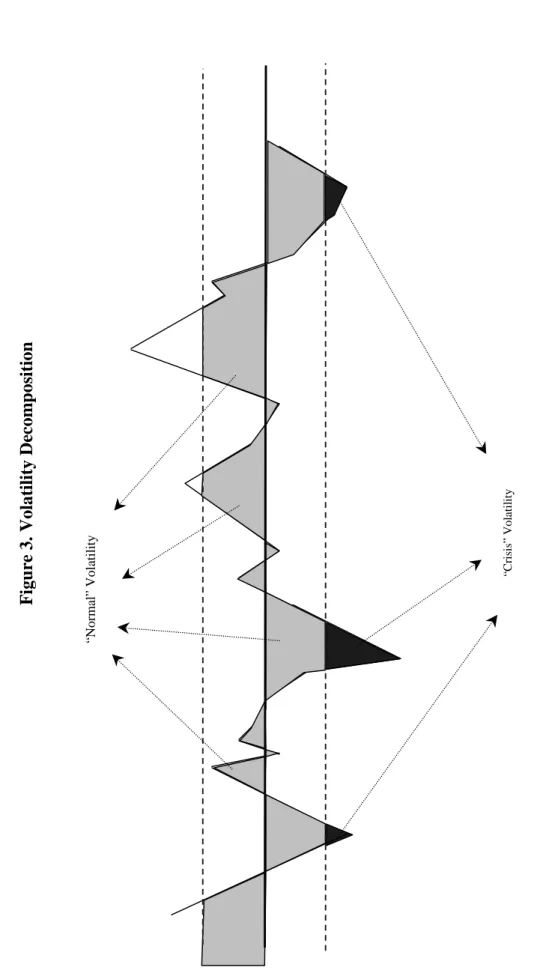
The measures of “normal” and “crisis” volatilities are obtained from the same distribution as the overall volatility measure. “Crisis” volatility is the portion of the standard deviation of GDP growth or output gap that corresponds to downward deviations below a certain threshold (see the example in Figure 3). This threshold is set equal to one standard deviation of the world distribution of overall volatility measures (thus, it is common to all countries). Using a common threshold generates absolute (as opposed to relative, country-specific) crisis measures and, thus, facilitates cross-country comparisons. “Normal” volatility is then defined as the portion of the standard deviation of GDP growth or output gap corresponding to deviations that fall within the threshold. Table 2 shows the cross-country correlations between the per capita GDP growth rate and the overall, “crisis,” and “normal” volatility measures. We observe that overall volatility is highly correlated (at least 80%) with any of its components, “crisis” or “normal.” The correlation coefficient between “crisis” and “normal” volatilities is around 55%, which is high enough to denote a strong link but not so high as to render one of them redundant. Including each of them in the analysis will provide independent informational content. Finally, note that the correlation between per capita GDP growth and the volatility measures is always negative, in the neighborhood of -35% for overall and “normal” volatilities, and around –23% for “crisis” volatility. The lower correlation between growth and the “crisis” component would indicate that, when competing as explanatory variables for growth, “normal” volatility would prevail. As we see at the end of next section, this is not the case.

Regarding the dependent variable, the rate of growth of GDP per capita is calculated as the annualized log difference of the period’s final and initial real GDP per capita. The control variables are the period’s initial level of real GDP per capita, the average ratio of domestic private credit to GDP, and the average secondary school enrollment ratio. The instrumental variables are calculated as follows. The volatility of inflation and terms of trade shocks are calculated as the standard deviation of,

respectively, the growth rates of the consumer price index and the terms of trade over the corresponding period. The measure of real exchange misalignment is calculated as the absolute difference of the real exchange rate and its equilibrium level --where this is obtained by fitting a country’s consumer purchasing power on its average income, population density, and region-specific factors. The frequency of banking crises is given by the ratio of years a country experienced a systemic banking crises to the total number of years in the period. See the appendix for more details on variable definitions and data sources.

III. RESULTS.

We now present the empirical results on the relationship between macroeconomic volatility and economic growth. For this purpose, we follow the outline explained in the methodological section.

A. Simple Correlations. Table 1 presents the bivariate correlation coefficients

between the two measures of volatility with each other and with the growth rate of GDP per capita for various samples of countries. For the full sample of countries the correlation between the growth rate and the two measures of volatility is negative. This is, however, not always the case for different sub-samples of countries. The correlation between volatility and growth appears to decline as average income decreases. It is in fact positive for high-income countries, close to zero for the medium-income group, and negative for low-income countries. A somehow different pattern emerges when we group countries according to financial development. The correlation between volatility and growth is positive for countries of high financial development. It becomes large and negative when we move to the medium group, and it remains negative but of smaller magnitude for low-financial-development countries. Therefore, when breaking the sample according to financial development, the correlations describe a nonlinear, “u” pattern.

In the case of trade openness, the correlations between volatility and growth are negative for all groups, but more so for medium- and highly-open economies. It would appear that the negative association between volatility and growth increases with openness. As we see later, this result does not survive the inclusion of additional

determinants for economic growth. When breaking the sample by the degree of institutional development, the pattern of correlations resembles that by income levels – that is, it becomes less negative as development occurs. However, in this case, the differences across groups are not as noticeable as when the sample is divided by income. Finally, when we split the sample by the degree of fiscal policy procyclicality, the correlation results are surprising: it would appear that highly procyclical countries have the smallest negative association between growth and volatility. This result is unexpected because procyclical fiscal policies tend to magnify the effect of macroeconomic shocks. However, as we see below, this result is upturned when we control for other growth determinants.

B. Regression Analysis: Homogeneous effect of volatility on growth. Table 3

presents the regression coefficients, associated t-statistics, and other estimation results for simple and multiple regressions of the growth rate of GDP per capita on the volatility measures (one by one) and the control variables.

The simple regression (Cols. 1 and 4) indicates a negative and statistically significant association between either measure of volatility and economic growth. The size and statistical significance of the volatility coefficient decline only marginally when we control for initial GDP per capita. In fact, after including our full set of controls, the volatility coefficient declines only slightly from its simple-regression value and retains its statistical significance at usual confidence levels. It appears, then, that the direct link between volatility and growth is not captured by the standard growth determinants.

The following sections consider, in turn, four avenues for a deeper study of the volatility-growth connection: first, the link between volatility and growth may change depending on the structure of the economy; second, volatility may be jointly endogenous with economic growth; third, the volatility-growth link may have changed over time; and fourth, large and negative fluctuations may explain the negative volatility-growth link.

C. Regression Analysis: Heterogeneous effect of volatility on growth depending on various country characteristics. In contrast to the previous set of

regressions, here we allow the empirical link between volatility and growth to vary according to some country structural characteristics. These are the overall level of development (proxied by the level of per capita income), the depth of financial markets,

the openness of international trade, the level of institutional development, and the degree of fiscal policy procyclicality. As explained in the methodological section, we can account for heterogeneous volatility-growth links through “continuous” and “categorical” interactions.

a. Continuous interaction effects. These effects are measured through the coefficient on the multiplicative term between each volatility measure and the proxy for a given structural characteristic. Table 4, panels A and B, reports these results. We find strong evidence that the level of (initial) income affects the relationship between volatility and growth, in the sense that it tends to be less negative for higher income countries (see Col. 1 in panels A and B). As is the case for most findings in the paper, the two measures of volatility render the same qualitative results. When we interact volatility with institutional development (see Col. 4 in panels A and B), we also find that the negative link between volatility and growth weakens in a statistically significant fashion.

In the case of financial depth (see Col. 3 in panels A and B), the coefficient on volatility remains negative but loses significance when we include the interaction term, which itself is positive but lacks statistical significance. As we see below, this doesn’t mean that nonlinear effects are unimportant in the case of financial depth. It only means that the volatility-growth relationship does not vary linearly with the level of financial development, as the correlation analysis had anticipated. In the case of fiscal procyclicality (see Col. 5 in panels A and B), the interaction term is negative, indicating that more procyclical fiscal policies worsen the negative link between volatility and growth. However, this result is significant --and marginally so-- only in the case of the standard deviation of GDP growth as the measure of volatility. As in the case of financial development this appears to indicate a more complicated pattern for the effect that fiscal policy procyclicality has on the volatility-growth link, as we see below. Finally, when we interact volatility with trade openness (see Col. 2 in panels A and B), we find that although the coefficient on volatility remains negative and statistically significant, that on the interaction is not significant. Contrary to the cases of financial development or fiscal procyclicality, the lack of significance of the trade interaction simply reflects the fact that openness has no impact on the volatility-growth relationship.

b. Categorical interaction effects. As mentioned above, the lack of significant results on some of the continuous interactions is that they impose a monotonic relationship between the volatility-growth link and a given structural characteristic (for instance, the effect of volatility on growth must decline, stay constant, or increase with financial development, but it cannot describe a non-monotonic, “u”-type of pattern). In this section, we allow for non-monotonic effects through categorical interactions.

Categorical interaction effects are measured through the coefficient on the multiplicative term between each volatility measure and the binary variable that indicates whether the country belongs or not to a given group. As explained in the methodological section, for each structural characteristic we divide the sample into three groups of similar size (groups of low, medium, and high values for the corresponding structural characteristic). We estimate the volatility coefficients for each of the three groups, which allows us to test whether each of them is statistically significant. In addition, we test whether the coefficients for the low and medium groups are different from the high group, which, therefore, acts as the benchmark. Table 5, panels A and B, reports the regression estimation results and related tests.

Regarding the level of income (Col. 1), we find that there is no significant relationship between volatility and growth for countries of medium and high income. In contrast, the volatility-growth link is significantly negative for poor countries. We find a similar result in the case of institutional development (Col. 4), that is, the relationship between volatility and growth is significantly negative only in the group of poorly developed countries. A likely interpretation for these results is that as countries develop they have the means --from stabilization policies, institutional safeguards, and insurance markets-- to neutralize the long-run effects of volatility (see Fatás 2002). Note that the volatility coefficient for medium countries is negative, as is for low countries, but fails to be significant. We return to this case when we control for the potential endogeneity of volatility.

Regarding financial development (Col. 3), there is no significant link between growth and volatility in countries that are either highly or poorly financially developed. However, there is strong evidence of a negative relationship for countries in the middle of the financial-development spectrum. This result is consistent with the literature that

indicates a larger macroeconomic vulnerability in countries that have just liberalized their financial systems (see Gaytán and Ranciere 2002). When we consider trade openness as the structural characteristic of interest (Col. 2), we find that the volatility coefficient is significantly negative in all country groups and that the differences across groups are not statistically different from zero. Together with the result on the continuous interaction, this indicates that openness has no bearing on the volatility-growth link; that is, open countries are as likely to deal with their volatile environment and neutralize it as closed economies are. Finally, when we classify countries by their degree of fiscal policy procyclicality (Col. 5), we find that only in countries that conduct relatively more counter-cyclical policies, volatility has no statistically significant link with growth (see Imbs 2002). This is particularly noticeable when volatility is measured as the standard deviation of GDP growth. Moreover, we find that the negative coefficient on volatility tends to be larger (although not statistically so) for medium than for high fiscal procyclical economies. One interpretation for this result is that medium countries are also the most uncertain regarding how governments react to shocks, and it is this uncertainty that worsens the volatility growth connection.

In sum, the types of countries where volatility and growth appear to be negatively related are the relatively poor, the institutionally underdeveloped, the more-or-less financially developed, and those that conduct mixed or highly procyclical fiscal policies. The level of openness does not appear to worsen or improve the negative relationship between volatility and growth.

D. Instrumental Variable Regression Analysis: Controlling for the joint endogeneity of volatility. Here we attempt to estimate the causal effect of volatility on

growth. We do so by extracting the exogenous component of volatility through the use of instrumental variables. We allow also for interaction effects (both continuous and categorical) but only related to level of income, the most relevant indicator of overall development. Table 6, panels A and B, reports the results when we don’t allow for interaction effects (Col. 1) as well as when we consider continuous (Col. 2) and categorical (Col. 3) interaction effects between volatility and level of income.

The set of instrumental variables used in the analysis consists of real exchange rate misalignment, frequency of banking crises, price volatility, proxied by the standard deviation of inflation rate, and volatility of terms of trade shocks.

Before discussing the estimation results, the first issue to consider is whether there are grounds to believe that the volatility measures may be subject to joint endogeneity. For this we conduct a Hausman-type test, reported at the bottom of Table 6. Under the null hypothesis that volatility is exogenous, the ordinary-least-squares (OLS) estimates are both consistent and efficient, and the instrumental-variable (IV) estimates are consistent but not efficient. In contrast, under the alternative hypothesis, only the IV estimates are consistent. The test results lead us to strongly reject the null hypothesis of exogenous volatility and points to the use of instrumental variables to estimate the causal impact of volatility on growth.

Next, we need to make sure that the instrumental variable procedure is appropriate. This depends on, first, whether the instrumental variables can explain a large share of the variation in volatility and, second, whether they are related to economic growth only through the explanatory variables in the regression (so that the instruments’ correlation with the regression residual is zero). In order to show the instrumental variables’ strong explanatory power on the volatility measures, we report the R-squared coefficients of the first-stage regression. They are about 50% in the first two columns and jump considerably when we allow for categorical interaction effects. The full first-stage regression (not reported) indicates that all instruments exhibit the expected positive coefficient, and all are statistically significant, except for the frequency of banking crises. Then, to assess whether the instrumental variables are not correlated with the regression residual we conduct a Hansen test of overidentifying restrictions and report its p-value. Fortunately, the test clearly indicates that we should not reject the hypothesis that there is no correlation between the instrumental variables and the error term.

The general result from the IV estimation is that the coefficient on volatility becomes larger in magnitude and stronger in statistical significance than the corresponding OLS estimate. Apparently, there is a positive association between volatility and growth that comes from either simultaneous causation from third variables or a positive feedback from growth to volatility. Once we remove this positive link, the

negative effect from volatility to growth is revealed to be larger in magnitude. In fact, comparing Table 6 (Col. 1) with Table 3 (Cols. 3 and 6), the IV volatility coefficients are more than twice as large as the OLS coefficients, whether we consider the standard deviation of the output gap or GDP growth as the measure of volatility. We discuss the economic significance of the estimated effect of volatility on growth in the concluding section.

When we consider income interaction effects (Cols. 2 and 3), it is also the case that the volatility coefficient under IV is larger than its OLS counterpart. This is particularly noticeable when we allow for categorical interactions. Now, we find that volatility has a negative impact on growth not only in poor countries but also in medium-income economies (although more so in the former group). Nevertheless, it is still the case that for rich countries volatility has no significant effect on growth.

E. Pooled regression analysis: The stability of the volatility-growth relationship over time. We now consider whether the link between volatility and

growth has changed in recent decades. As explained in the methodological section, for this purpose we conduct pooled regression analysis on country observations corresponding to the four decades since the 1960s to the 90s. We carry out the analysis first ignoring and then allowing for income interactions, and the results are reported in Tables 7 and 8, respectively. In both cases, we obtain the regression coefficients through OLS and IV estimators.

Let’s first consider the results in Table 7, which ignore income interactions. For both OLS and IV estimators, the largest volatility coefficients belong to the 1980s. Focusing on the IV estimates, there is a sharp and statistically significant increase in the size of the volatility effect on growth from the 1960s to the 70s and even further to the 80s. The 1990s coefficient is only a little smaller than that of the 1980s, and the difference is not statistically significant. The marked change between the first two decades and the latter two does not appear to be related to a change in the cross-country mean or variance of either volatility measure. What seems to drive the change is the substantial decrease in the mean growth rate, which dropped to less than one third from the 1960s to the 80s and less than one half from the 1960s to the 90s. The world is not more volatile now than 30 years ago, but volatility is taking a larger toll on growth.

Table 8 tells a similar story, implying that the volatility interaction with income cannot explain the changes in recent decades. The coefficients on volatility and on the income interaction term are remarkably similar between the 1960s and 70s, and also between the 1980s and 90s; but a break occurs in the 1980s, and the difference between the first two decades and the latter two is notable and statistically significant. The fact that the coefficients on volatility and on the interaction term change by roughly the same proportion indicates that the overall growth effect of a change in volatility also changes proportionally, provided income stays constant. The gains from an increase in income --in terms of a dim--inished --indirect effect of volatility on growth-- are larger --in the latter decades but so is volatility’ negative direct effect.

F. Regression Analysis: Volatility and Crises. It can be shown that a high

measure of volatility can result from large but infrequent swings in per capita GDP as from small but frequent fluctuations. However, their respective real effects could be sharply different (see Caballero 2002). The measures of volatility we have used up to now in the paper combine normal and crisis fluctuations. In this section, we work with the components of volatility to answer the last question we pose in this paper. This is whether the negative relationship between volatility and growth is actually due to the harmful impact of large negative fluctuations (“crisis” volatility) and not really to the effect of repeated but small fluctuations around the trend (“normal” volatility).

We take the basic model (Table 3, Cols. 3 and 4) and replace overall volatility by measures of “normal” and “crisis” volatilities. Then we estimate the model by OLS and IV estimators. The results are reported in Table 9. We find that although both forms of volatility present negative coefficients, only “crisis” volatility is statistically significant. This is true whether we work with the output gap or per capita GDP growth as the proxy for macroeconomic fluctuations; although the contrast between “crisis” and “normal” volatility effects is sharper in the case of the output gap. As before, the IV estimates render larger coefficients for either type of volatility, but only the “crisis” one is statistically significant. In the case of the output gap, the effect of “crisis” volatility is almost twice as large as that of overall volatility (compare Table 6, panel A, Col. 1 with Table 9, Col. 2).

IV. CONCLUSIONS.

Analyzing cross-country data, we conclude that macroeconomic volatility and long-run economic growth are negatively related. This negative link is exacerbated in countries that are poor, institutionally underdeveloped, undergoing intermediate stages of financial development, or unable to conduct countercyclical fiscal policies. On the other hand, the volatility-growth association does not appear to depend on a country’s level of international trade openness.

Furthermore, the negative global relationship between macroeconomic volatility and long-run growth actually reflects an even stronger, harmful effect from volatility to growth. This is true for a worldwide sample of countries, and particularly so in low and middle-income economies. The negative effect of volatility to growth has been present since the 1960s, but it has become considerably larger in the last two decades. This is not due to a change in volatility trends over time but, rather, to the reduction in growth in the 1980s and 1990s and the countries’ inability to deal with volatility in that context.

Examining the components of volatility, we find that its negative impact on growth is not the effect of small although repeated cyclical deviations but to large drops below the output trend. Therefore, it’s the volatility due to crisis, and not due to normal times, that harms the economy’s long-run growth performance.

The effects we have just described are not only statistically significant; rather, their magnitude leads us to believe that they are also economically significant. In order to illustrate volatility’s long-run impact, Table 10 reports the growth effect of a change in volatility under various conditions. In order to make the table figures comparable with each other, we apply in all exercises the same benchmark change in volatility. We set it equal to one worldwide, cross-country standard deviation of volatility, which for each country is measured as the standard deviation of the output gap over 1960-2000. To make this benchmark change in volatility more concrete, consider the following two examples of sequences of countries. In each sequence, countries are presented in ascending order of volatility, and the separation between two consecutive countries is about one standard deviation of volatility. The first example sequence, which covers almost the full spectrum of countries in the sample, is, France, Egypt, Uruguay, Jordan,

and Nigeria. The second example, which covers countries towards the middle of the volatility distribution, is, Japan, Botswana, and Argentina.

If we ignore the endogeneity of volatility, the growth decline due to a one-standard-deviation increase in volatility appears to be modest, at about 0.5 percentage points of the growth rate. However, once we account for simultaneous and reverse causation in the volatility-growth relationship, the same increase in volatility is found to lead to a 1.3 percentage-point drop in the growth rate, which already represents a sizeable loss. This decline in growth is magnified even further if we consider the same change in volatility in the 1990s or under a crisis situation. In both cases, the loss would amount to about 2.2 percentage points of the per capita GDP growth rate. For the government and the private sector alike, macroeconomic volatility should be not only a source of short-run concerns but also a constant preoccupation for the achievement of long-short-run goals.

REFERENCES

Alesina, A., Ozler S., N. Roubini, and P Swagel (1996). “Political Instability and Economic Growth,” Journal of Economic Growth 2: 189-213.

Aghion, P. and G. Saint-Paul (1998). “Virtues of Bad Times: Interaction between Productivity Growth and Economic Fluctuations”. Macroeconomic Dynamics 2 (3): 322-344.

Barro, R. J. (1991). “Economic Growth in a Cross Section of Countries”. Quarterly

Journal of Economics 106 (2): 407-443.

Baxter, M. and R.G. King (1999). “Measuring Business Cycles: Approximate Band-Pass Filters for Economic Time Series.” The Review of Economics and Statistics 81: 575-593. Bertola, G. and R. J. Caballero (1994). “Irreversibility and Aggregate Investment”. The

Review of Economic Studies 61 (2): 223-246.

Caprio, G. and D. Klingebiel (1999). “Episodes of Systemic and Borderline Financial Crises”. World Bank. Mimeo.

Caballero, R. J. and M. L. Hammour (1994). “The Cleansing Effect of Recessions” The

American Economic Review 84 (5): 1350-1368.

Caballero, R.J. and M. L. Hammour (1996). “On the Timing and Efficiency of Creative Destruction” The Quarterly Journal of Economics 111 (3): 805-852.

Caballero, R. J. (2000). "Macroeconomic Volatility in Latin America: A View and Three Case Studies," Economia 1(1): 31-108. Reprinted in Estudiosde Economia 28(1), June 2001, 5-52.

Caballero, R. J. (2001). “Macroeconomic Volatility in Reformed Latin America:

Diagnosis and Policy Proposals”. Washington, D.C.: Inter-American Development Bank. Caballero, R. J. (2002). “Coping with Chile’s External Vulnerability: A Financial

Problem,” Economic Growth: Sources, Trends, and Cycles, Banco Central de Chile, edited by Norman Loayza and Raimundo Soto. 377-416.

Easterly, W., R. Islam and J. E. Stiglitz (2000). “Shaken and Stirred: Explaining Growth Volatility”. In The World Bank Annual Conference on Economic Development, Washington, D.C.

Fatás, A. (2000a). “Endogenous Growth and Stochastic Trends.” Journal of Monetary

Economics 45, 107-128.

Fatás, A. (2000b). “Do Business Cycles Cast Long Shadows? Short-run Persistence and Economic Growth.” Journal of Economic Growth 5: 147-162.

Fatás, A. (2001). “The Effects of Business Cycles on growth.” Unpublished manuscript. INSEAD.

Fatás, A. (2002). “The Effects of Business Cycles on Growth.” Central Bank of Chile Working Paper No. 156, May.

Fischer, S. (1993). “The Role of Macroeconomic Factors in Growth.” Journal of

Monetary Economics 32 (3): 485-511.

Hall, R. E. (1991). “Labor Demand, Labor Supply, and Employment Volatility,” NBER

Macroeconomics Annual: 17-46.

Hall, R. E. (1993). “Macro Theory and the Recession of 1990-1991 (in What Caused the Last Recession?)”. The American Economic Review, 83 (2), Papers and Proceedings of the Hundred and Fifth Annual Meeting of the American Economic Association: 275-279. Imbs, J. (2002). “Why the Link between Volatility and Growth is both Positive and Negative”. CEPR Discussion Papers No. 3561.

IMF (2002). World Economic Outlook. International Monetary Fund, April. Washington, D.C.

Judson, R. and A. Orphanides (1996). “Inflation, Volatility and Growth”. Washington, Board of Governors of the Federal Reserve Bank, Finance and Economics Discussion

Series No. 19.

Kroft, K. and H. Lloyd-Ellis (2002). “Further Cross-Country Evidence on the link Between Growth, Volatility and Business Cycles”. Queens University Working Paper. Levine, R. and D. Renelt (1992). “A Sensitivity Analysis of Cross-Country Growth Regressions”. American Economic Review 82 (4): 942-63.

Martin, P. and C. A. Rogers (1997). "Stabilization Policy, Learning By Doing, and Economic Growth". Oxford Economic Papers.

Martin, P. and C. A. Rogers (2000). “Long-term growth and short-term economic instability”. European Economic Review 44 (2): 359-381.

Mills, T. C. (1999). “Business Cycle Volatility and Economic Growth: A Reassessment”. Manuscript, Loughborough University.

Ramey, G. and V. Ramey (1995). “Cross-Country Evidence on the Link between Volatility and Growth”. American Economic Review 85 (5): 1138-1150.

Ranciere, Romain and Alejandro Gaytán (2002). “Banks, Liquidity Crises, and Economic Growth.” Mimeo. New York University.

Rodrik, D. (1991). "Policy Uncertainty and Private Investment in Developing Countries".

Journal of Development Economics 36.

Schumpeter, J. A. (1939). “Business Cycle: A Theoretical, Historical, and Statistical Analysis of the Capitalist Process”. New York: McGraw-Hill.

Serven, L. (2003). “Real-Exchange-Rate Uncertainty and Private Investment in LDCs”.

Review of Economics and Statistics 85 (1): 212-218.

Shleifer, A. (1986). “Implementation Cycles”. Journal of Political Economy 94 (6): 1163-1190.

Summer, L. and A. Heston (1991). “The Penn World Table (Mark 5): An Expanded Set of International Comparisons, 1950-1988.” Quarterly Journal of Economics 106(2): 327-68.

Talvi, E. and C. A. Végh (2000). “Tax base variability and procyclical fiscal policy”.

NBER Working Paper No. 7499.

TIMSS (2000). The TIMSS 1999 International Database. Boston, Mass: Boston University.

Wolf, Holger (2003). Introductory Chapter. This Volume.

World Bank (1997). World Development Indicators, Washington, DC: The World Bank. World Bank (2000). World Development Indicators, Washington, DC: The World Bank. World Bank (2002). Global Economic Prospects. Washington, D.C.

Appendix

Definitions and Sources of Variables Used in Correlation and Regression Analysis

Basic Variables Definition and construction Source

Real per capita GDP (in 1985 US$ PPP) Ratio of total GDP to total population.

GDP is in 1985 PPP-adjusted US$. Growth rates are obtained from constant 1995 US$ per capita GDP series.

Authors' construction using Summers, Heston and Aten (2002) and The World Bank (2002).

Output gap Difference between the log of actual

GDP and (the log of) potential (trend) GDP. In order to decompose the log of GDP, the Baxter-King filter is used.

Authors’s calculations.

Gross secondary-school enrollment Ratio of total secondary enrollment,

regardless of age, to the population of the age group that officially corresponds to that level of education.

World Development Network (2002) and The World Bank (2002).

Domestic Credit to the Private Sector (% of GDP)

Ratio to GDP of the stock of claims on the private sector by deposit money banks and other financial institutions.

Beck, Demirguc-Kunt and Levine (2000).

Trade Openness (% of GDP) Ratio of exports and imports (in 1995 US$)

to GDP (in 1995 US$).

World Development Network (2002) and The World Bank (2002).

Structural Variables

Index of Institutional Development First principal component of four

indicators: prevalence of law and order, quality of bureaucracy, absence of corruption, and accountability of public officials.

International Country Risk Guide (ICRG)

Government Consumption (% of GDP) Ratio of government consumption to

GDP.

Summers, Heston and Aten (2002)

Fiscal Policy Procyclicality Correlation between GDP growth rate

and growth rate of the government consumption.

Instrumental Variables

Volatility of Inflation Measured by the standard deviation of

the rate of change in the consumer price index: annual percentage change in the cost to the average consumer of acquiring a fixed basket of goods and services.

The World Bank (2002).

Real Exchange Rate Misalignment Absolute deviation of the real exchange

rate overvaluation from the equilibrium real exchange rate (set to 1).

The extent of Real Exchange Rate disequilibrium is defined as the difference between actual real effective exchange rate and its equilibrium level, given by cross-country purchasing power parity comparisons.

Loayza and Kubota (2003)

Systemic Banking Crises Number of years in which a country

underwent a systemic banking crisis, as a fraction of the number of years in the corresponding period.

Authors’s calculations using data from Caprio and Klingebiel (1999), and Kaminsky and Reinhart (1998).

Volatility of Terms of Trade shocks Standard deviation of the log difference

of the terms of trade.

The World Bank (2000) "World

26 Ta b le 1 : S im p le C o rrel a ti on s C ro ss-S e c tio na l A n a ly s is S a m p le : 79 c o u n tr ie s, 1 9 6 0 20 00 Av era g e G D P per c a pita St and a rd De v iat io n o f Gr o w th an d : Ou tp u t Gap an d: N. Ob s. St an da rd D e v ia ti o n o f St an dard D e viat ion o f St an dar d D e viat ion of Ou tp ut G a p G D P Pe r Capita G rowth G D P Per Cap it a G row th Fu ll S a m p le 79 -0. 353 8 -0 .3 45 0 0. 98 04 By I n com e: Hig h I n c o m e 22 0 .45 58 0. 60 43 0. 89 47 ( O EC D co u n tr ie s+ Is ra e l) Mid d le In co me 34 0 .03 56 0. 05 40 0. 98 07 ( u ppe r- an d lo wer-m iddl e in c o me c o u n tr ies ) Lo w I n c o m e 23 -0. 385 2 -0 .4 42 5 0. 96 73 ( lo w in c o m e co u n tr ie s) By Fin a n c ial D e v e lopm e n t: H igh Fi na nc ia l D e v e lo p m e n t 26 0 .25 42 0. 26 91 0. 97 83 (c o u n tr ies w it h p ri v a te do m e st ic cr ed it /GDP > 4 1 % ) Me diu m F in a n c ial D e v e lo pme n t 26 -0. 493 6 -0 .4 44 8 0.98 ( c o u n tr ies w it h p ri v a te do m e st ic cr ed it /GDP > 2 1 % A n d <4 1% ) Lo w Fi na nc ia l D e v e lo p m e n t 27 -0. 254 3 -0 .2 47 3 0. 97 03 (c o u n tr ies w it h p ri v a te do m e st ic cr ed it /GDP < 2 1 % ) By T rad e Open nes s : Hig h T rade O p e n n e ss 26 -0 .4 17 -0 .3 78 7 0. 97 7 ( c o u nt ri e s w ith tr a d e v o lu m e / G DP > 7 1 % ) Me d iu m Tr ad e O p e n n e ss 26 -0 .4 84 -0 .4 75 8 0. 99 52 ( c o u nt ri e s w ith tr a d e v o lu m e / G DP > 4 5 % A n d < 7 1 % ) Lo w T ra d e Op e nne ss 27 -0. 149 5 -0 .1 56 3 0. 96 73 ( c o u nt ri e s w ith tr a d e v o lu m e / G DP < 4 5 % ) By I n s titu tion a l D e velo p m en t: Hig h L e ve l o f In st it u tio n a l De ve lo pm en t 26 0 .11 18 0. 28 15 0. 94 47 ( a b o ve 5 7 % o f I C R G i n d e x r a n g e) Me diu m L e vel o f I n st it u tio n a l De vel o pm en t 26 -0. 138 3 -0 .1 41 7 0. 96 64 ( b e tw e en 3 6 % A n d 5 7 % o f I C R G i n d e x r a n g e) L o w L e ve l o f In st it u tio n a l D e ve lo pme n t 27 -0. 193 3 -0 .2 35 5 0. 98 29 ( b e lo w 3 6 % o f I C R G i n d e x r a n g e) By Degree of Fis c al P o licy Procyc lic a lit y: Hig h ly P ro c y c lic al F is c a l P o licy 26 -0. 075 6 -0 .1 40 2 0. 98 47 ( c o rr [ Y , GC ] > -1 0 %) M e di um Pro c y c lic a l F isc a l Po li c y 26 -0. 587 5 -0 .5 50 6 0. 97 74 ( c o rr [ Y , GC ] -2 4 % > A n d < -10 %) C o u n te r-c y clic al F is c al P o licy 27 -0. 325 3 -0 .2 76 3 0. 98 34 ( c o rr [ Y , GC ] < -2 4 %) Sou rc e : A u th ors' s c a lc u la ti o n s

27 2: Si mple C o rr el ation s w it h “com pon e n ts ” of St d. D e v ia tion s-S ect io n a l A n a lys is p le : 79 cou n tr ie s, 1 960 200 0 (A) . Vo lat ility: Me an Gr o w th Stan dard De v ia tio n o f Outpu t G a p Aggre gate Vo latility "C risis" Vo latilit y "N o rmal" Vo la tility n G ro w th 1 ggr e g ate V o latil ity: s td de v o f o u tp u t gap -0 .3 5 3 8 1 C ris is" V o lat ilit y : std de v o f ou tp u t ga p -0 .2 4 2 3 0. 85 38 1 N o rmal" V o lat ilit y : s td de v of o u tput gap -0 .3 5 3 7 0. 90 56 0.6 0 4 1 1 (B). Vo latilit y: Standa rd De v iatio n o f G D P Pe r C a p ita G ro w th Aggre gate Vo latility "C risis" Vo latilit y "N o rmal" Vo la tility ggre g at e V o lat ilit y : s td de v o f GD P pe r c a pita gro w th -0 .3 4 5 1 ri sis " V o lat ility : s td de v of G D P pe r cap ita gro w th -0 .2 2 8 4 0. 80 61 1 o rmal" V o latil ity : s td de v o f G D P pe r capit a gro w th -0 .3 5 5 4 0. 88 31 0.5 2 4 9 1 c e : A u tho rs's c a lc u lati o ns

28 e 3 : H o mog e neous E ff ect o f Volat ility on Gro w th ss-Sec tional R e gr essi on A n aly sis, 19 60 - 2 000 D e p e nd en t V a ri a b le: Gr o w th R ate o f GDP p e r c api ta (A ) Vo lati li ty: (B ) V o lat il it y : S tan dar d De v iati o n o f Out p ut Ga p S tan dar d De v iati o n o f GD P P e r Cap ita Gr o w th [1] [2] [3] [4] [5] [6 ] tility -0. 5507 -0 .4996 -0 .4383 -0.3355 -0 .2994 -0. 2605 -2. 8 9 -2 .6 3 -3 .2 4 -2.87 -2 .5 7 -3. 0 2 l V a ria b le s: G D P P e r C a pi ta 0.0672 -0 .9358 0.0759 -0. 9276 o g s) 0.57 -5 .8 9 0. 64 -6. 0 1 a ti o n 1. 6119 1. 6188 on d a ry enrol lm ent , i n l o gs) 4. 89 4. 92 nci a l D e p th 1. 1664 1. 1617 a te d o me st ic cre d it/G DP, in lo gs ) 4. 37 4. 48 u a red 0. 1251 0.1274 0. 5823 0. 1190 0.1219 0. 5772 n tr ie s / No. O b se rv at ion s 79 / 79 79 / 79 79 / 79 79 / 79 79 / 79 79 / 79 s: t -St a ti st ics a re present e d b e lo w t h e correspon d ing coeff ici en t e rc ep t i s i n cl u d ed i n a ll es ti m a ti ons but n o t report ed ta n d a rd error s a re correct ed for p o te nt ia l het e rosced a st ici ty u si n g N e w e y-West proced u re e : A u tho rs' es ti m a tio n

29 Heter o ge neou s E ffect of V o la ti li ty o n G rowt h , C o n ti n uou s In ter a ct ion E ffect s S e c tio n a l R e gr e ssi o n A n al y si s, 1960 200 0 De pe nde n t Var ia b le : G rowt h R a te of G D P p e r c a p it a (A ) V o la ti li ty : S tan d a rd D e v iat io n o f Ou tp u t Ga p V o latilit y Int e rac ted w ith: In c o m e Tr a d e O p en n e ss Fi n . D e v e lo p m e n t Ins tit. De v e lo pmen t F is c al P o lic y P ro c y c lic ality [1 ] [2 ] [3 ] [4 ] [5 ] y -2 .4 41 7 -0 .332 1 -0 .8 258 -0 .2 34 1 -0 .4 369 ard de v iati o n o f ou tpu t ga p) -3 .2 -2 .1 6 -1 .4 3 -1 .9 1 -3 .0 8 y Int e rac tion 0.291 2 -0 .001 4 0.11 88 0 .21 16 -0 .2 190 tility *c o rre spo n d ing s tru c tu ral variable ) 2. 9 2 -1 .2 4 0. 71 3. 7 2 -1 .3 5 able s: D P P e r C a pita -1 .3 90 4 -0 .942 5 -0 .8 833 -1 .1 63 8 -0 .9 508 -5 .7 9 -6 .0 9 -5 .0 7 -6 .6 3 -5 .5 4 io n 1.283 5 1. 62 07 1.58 27 1 .83 83 1.63 78 n d a ry en rollm ent, in lo g s) 3. 8 7 4.94 4. 55 5. 8 8 4. 8 9 ial De pt h 1.163 0 1. 14 93 0.82 89 0 .69 35 1.18 29 te d o me st ic c re d it /G D P , in lo g s) 4. 4 4.28 1. 85 2. 6 2 4. 3 4 red 0.651 5 0 .58 76 0.58 51 0 .67 51 0.59 27 u n tr ie s / No . O b se rv a ti o n s 79 / 79 7 9 / 7 9 79 / 79 79 / 79 79 / 79 t -St a ti st ics a re p rese n te d b e lo w t h e c o rr e sp on d in g c o e ff ic ien t In te rc ep t i s i n cl ude d i n a ll e st im a ti o n s b u t no t rep o rt e d a n da rd e rro rs a re c o rre ct ed fo r p o te n ti a l h e te ro sc eda st ici ty us in g N e w e y-W e st p ro c e d ure u thor s' e sti m a ti on

30 : Heter o g e n e ou s Ef fec t o f Volatilit y on G row th , Co n tin u o u s In teraction E ffects (c on t. ) s-S ect io n a l R e gr e ss ion An al y si s, 1 9 60 - 20 00 De p e nd e n t Var iabl e : Grow th R a te of G D P p e r ca p it a (B ) Vo la til ity : St andar d D e v iati o n o f GDP Pe r C a p ita G ro w th Vo la ti lity Inte ra c te d with: In c o m e Tr a d e O p en n e ss Fi n. D e ve lo pm ent In st it . De ve lo p m en t F is c a l Po licy Pr o c yc lica lit y [1 ] [2 ] [3 ] [4 ] [5 ] ti lity -1 .6 7 4 6 -0. 2 01 5 -0. 5 15 8 -0. 1 13 9 -0. 2 60 5 ndar d dev iat io n of G D P pe r c a pi ta gro w th ) -3. 6 2 -1 .9 6 -1 .3 5 -1 .3 2 -2 .9 5 ti lity Inter a c tio n 0. 2 064 -0. 0 00 7 0 .07 89 0 .13 86 -0. 1 51 9 at ili ty *c o rr e spo ndi n g st ru c tu ral var iabl e ) 3. 33 -0 .9 9 0.7 2 3.7 4 -1 .5 5 tr o l Var iabl e s: l G D P P e r C a p ita -1 .4 3 4 2 -0. 9 31 0 -0. 8 71 5 -1. 1 55 6 -0. 9 42 8 o gs) -6. 2 9 -6 .1 5 -4 .9 6 -6 .7 3 -5 .6 7 a tio n 1. 2 356 1. 626 9 1 .59 00 1 .84 37 1 .63 97 o n d a ry enr o llm e n t, i n l o g s) 3. 84 4.9 6 4.5 5 5.9 0 4.9 2 ial D e pth 1. 0 990 1. 146 7 0 .78 73 0 .63 37 1 .18 39 va te d o mes tic c re d it /GDP , i n l o g s) 4. 20 4.3 8 1.6 6 2.3 7 4.5 0 a re d 0. 6 658 0. 580 8 0 .58 05 0 .68 13 0 .59 06 u n tr ie s / No . O b se rv a ti o n s 79 / 79 79 / 7 9 79 / 7 9 79 / 7 9 79 / 7 9 s: t-St a ti st ics a re p res en te d b e lo w t h e co rr esp o n d in g co ef fi ci en t I n te rc e p t i s in c lu d e d i n al l e st im a ti o n s bu t n o t r e por te d St an dard e rr o rs are c o rr e c te d fo r pot e nt ia l he te ro sc e d as ti c it y u si n g Ne w e y -W e st pr oc e d u re A u th o rs' estim a ti o n