On the relationship between
satisfiability and partially observable
Markov decision processes
by
Ricardo Salmon
A thesis
presented to the University of Waterloo in fulfillment of the
thesis requirement for the degree of Doctor of Philosophy
in
Computer Science
Waterloo, Ontario, Canada, 2018
c
Examining Committee Membership
The following served on the Examining Committee for this thesis. The decision of the Examining Committee is by majority vote.
Supervisor(s): Pascal Poupart
Professor, Dept. of Computer Science, University of Waterloo
Internal Member: Peter van Beek
Professor, Dept. of Computer Science, University of Waterloo Jesse Hoey
Professor, Dept. of Computer Science, University of Waterloo
Internal-External Member: Mark Crowley
Professor, Dept. of Electrical and Computer Engineering, University of Waterloo
External Examiner: Fangju Wang
I hereby declare that I am the sole author of this thesis. This is a true copy of the thesis, including any required final revisions, as accepted by my examiners.
Abstract
Stochastic satisfiability (SSAT), Quantified Boolean Satisfiability (QBF) and decision-theoretic planning in finite horizon partially observable Markov decision processes (POMDPs) are all PSPACE-Complete problems. Since they are all complete for the same complexity class, I show how to convert them into one another in polynomial time and space. I discuss various properties of each encoding and how they get translated into equivalent constructs in the other encodings. An important lesson of these reductions is that the states in SSAT and flat POMDPs do not match. Therefore, comparing the scalability of satisfiability and flat POMDP solvers based on the size of the state spaces they can tackle is misleading.
A new SSAT solver called SSAT-Prime is proposed and implemented. It includes im-provements to watch literals, component caching and detecting symmetries with upper and lower bounds under certain conditions. SSAT-Prime is compared against a state of the art solver for probabilistic inference and a native POMDP solver on challenging benchmarks.
Acknowledgements
I would like to personally thank my supervisor, Dr. Pascal Poupart, for his guidance and support else this thesis would not be possible. We had many intense meetings fleshing out ideas on the whiteboard that were instrumental in narrowing the scope of my work. Also, special recognition to my committee members Dr. Peter van Beek, Dr. Jesse Hoey, Dr. Mark Crowley, and Dr. Fangju Wang for their time.
I would also like to show appreciation to all the friends I have made during my time in Waterloo, including members of the Hopeless Experts soccer team and the Computer Science GSA. A special thank you to Cristina and Jimmy that have kept me grounded and motivated through the good and bad times. Thanks to my brother, Shane, my mother, Sandra, and close family for their support in my journey here.
Finally, I would like to thank the following organizations for providing financial support. These include the University of Waterloo, Cheriton School of Computer Science, Canadian Natural Sciences and Engineering Council (NSERC), Ontario Graduate Scholarship (OGS), Mitacs Accelerate, Kik Interactive, Hockeytech, and Vector Institute.
Dedication
I dedicate this dissertation to Wayne Erdman, my high school teacher, for his encourage-ment. He was a tremendous teacher and mentor who inspired my pursuit of Mathematics, Computer Science, and higher education.
Table of Contents
List of Figures xi
List of Tables xii
1 Introduction 1 1.1 Contributions . . . 2 1.2 Outline. . . 3 2 Background 4 2.1 POMDP . . . 4 2.1.1 Value Function . . . 5 2.1.2 Value Iteration . . . 6 2.1.3 Approximations . . . 7 2.2 Satisfiability . . . 10 2.2.1 Boolean Satisfiability . . . 10
2.2.2 Quantified Boolean Formula . . . 12
2.2.3 Stochastic Satisfiability . . . 13
2.3 Probabilistic Inference . . . 14
2.3.1 Bayesian Network . . . 14
2.3.2 Inference Problems . . . 14
2.3.4 Marginal MAP . . . 16 2.3.5 Inference Algorithms . . . 16 2.3.6 Discussion . . . 18 2.4 Summary . . . 19 3 Related Work 20 3.1 POMDP Encoding . . . 20 3.2 Model Counting . . . 21 3.2.1 Encoding . . . 21 3.2.2 Local Structure . . . 23
3.3 Probabilistic Planning Solvers . . . 26
3.3.1 Zander . . . 26
3.3.2 DC-SSAT . . . 27
3.3.3 APPSAT . . . 28
4 Encoding Problems into POMDP 29 4.1 SAT ⇒ POMDP . . . 29
4.2 QBF ⇒POMDP . . . 32
4.3 SSAT ⇒ POMDP. . . 35
4.4 Discussion . . . 39
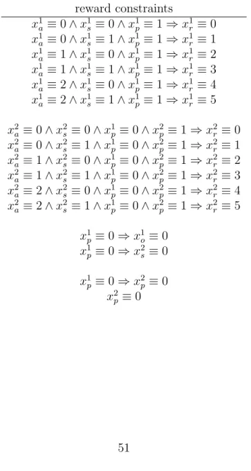
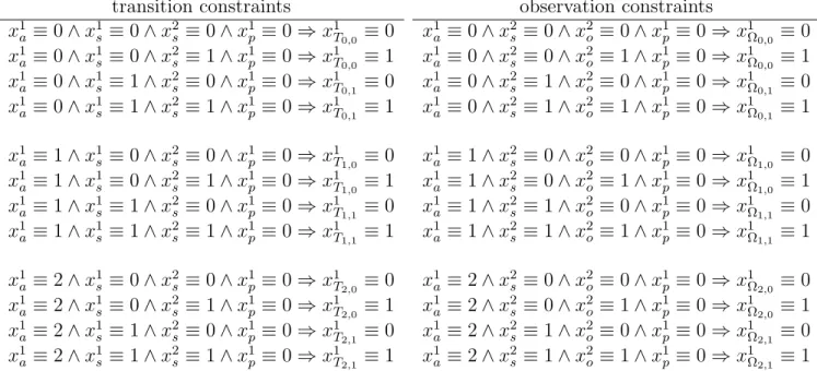
5 Encoding Problems into SSAT 40 5.1 POMDP ⇒ SSAT. . . 40 5.1.1 Example . . . 49 5.2 Summary . . . 53 5.3 Inference ⇒ SSAT . . . 54 5.3.1 Example . . . 54 5.4 Summary . . . 56
6 SSAT Solver 57
6.1 Finite Domain . . . 57
6.2 Unit Rule . . . 57
6.2.1 Two-Literal Watch Scheme. . . 58
6.2.2 Improved Watch Literal Scheme . . . 60
6.3 Component Decomposition . . . 63 6.3.1 Example . . . 64 6.4 Component Caching . . . 65 6.4.1 LRU Cache . . . 65 6.4.2 LRU-sizeof Cache . . . 65 6.5 Symmetry . . . 66 6.5.1 Canonical Representation . . . 66 6.5.2 Component Projection . . . 68
6.6 Branch and Bound . . . 69
6.7 Summary . . . 69 7 Experiments 71 7.1 Improvements . . . 71 7.1.1 Unit Rule . . . 72 7.1.2 Component Caching . . . 73 7.1.3 Symmetry . . . 75 7.1.4 Upper Bound . . . 75 7.1.5 Extra Techniques . . . 77 7.1.6 Summary . . . 78 7.2 Inference Competition . . . 79 7.2.1 Results . . . 79 7.2.2 Summary . . . 79 7.3 POMDP Benchmarks . . . 81
7.3.1 Results . . . 81 7.3.2 Summary . . . 83 7.4 Satisfiability Benchmarks . . . 83 7.5 Random Satisfiability . . . 83 7.5.1 Results . . . 84 7.5.2 Summary . . . 86 7.6 Conclusion . . . 87
8 Conclusion and Future Work 89 8.1 Conclusion . . . 89
8.2 Future Work . . . 90
8.2.1 Improve Solver Efficiency. . . 90
8.2.2 Changing the Encoding space . . . 92
References 94 APPENDICES 102 A Stationary Encoding of SAT 103 A.1 SAT⇒ POMDP . . . 103
A.2 Theorem . . . 105
List of Figures
3.1 A 3-variable Bayesian network. . . 22
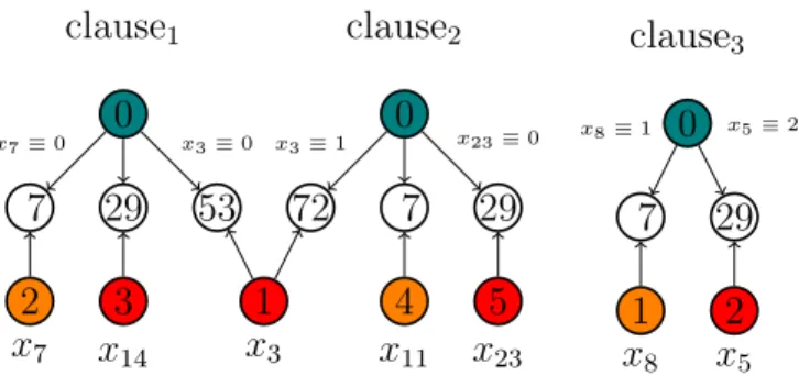
6.1 Watch literals for a clause when making the assignments x74 = 0, x3 = 1, x22= 0, x53= 2. Orange is watch literal 1 and teal is watch literal 2. . . 59 6.2 The constrained graph of a problem decomposed into a joint set of components. 64
6.3 Representation of Eq. (6.3.1) in canonical form. . . 68
6.4 Components of Eq. (6.3.1) in canonical form after assigning x3. . . 68 7.1 Convergence of lower and upper bound on two probabilistic problems. . . . 77
7.2 Cumulative time on inference benchmark from 2008 Competition . . . 80
7.3 The number of steps and probability of satisfiability for stochastic 3-SAT, 4-SAT, and 5-SAT problems . . . 85
7.4 The difficulty threshold for stochastic 3-SAT, 4-SAT, and 5-SAT problems 86
7.5 The number of steps and the probability of satisfiability for stochastic SAT for variables with increasing number of values. . . 87
List of Tables
3.1 Conditional distribution for random variables A, B, and C from Fig 3.1 . . 22
3.2 Parameter generated clauses for encoding Fig 3.1. . . 24
3.3 Weights for the CNF encoding of Fig 3.1. . . 24
4.1 beliefs in SAT example after taking actions x1 = f alse, x2 = f alse, x3 = f alse, x4 =true and x5 =true. . . 31
4.2 intermediate (unnormalized) beliefs in QBF example after processing a0 = (x1 := f alse), o1 = (x2 := f alse), a1 = (x3 := f alse), o2 = (x4 := true) and a3 = (x5 :=true). . . 35
4.3 intermediate (unnormalized) beliefs in SSAT example after processing a0 = (x1 :=f alse),o1 = (x2 :=f alse),a1 = (x3 :=f alse),o2 = (x4 :=true) and a3 = (x5 := true) where Pr(o1 = (x2 :=true)) = 1/6 and Pr(o2 = (x4 := true)) = 6/7. . . 38
5.1 The parameters for the tiger POMDP problem with normalized rewards. . 49
5.2 Example encoding of the Tiger problem from Table 5.1 for a horizon of length 2. . . 51
5.3 Example encoding of the transition and observation distributions in the Tiger problem from Table 5.1 for a horizon of length 2. . . 52
5.4 Conditional distribution for random variables A, B, and C. . . 55
5.5 Example encoding of the Bayesian network in Table 5.4. . . 55
7.1 Basic information for each benchmark problem. . . 72
7.3 Different improvements to the cache. . . 74
7.4 Results for improvement in symmetry by Canonical and Projection relabeling. 76
7.5 Basic information for each benchmark type. . . 78
7.6 The composition of the 251 problems in the Relational benchmark from the Inference competition. . . 79
7.7 Solving POMDP problems with a native solver PRUNE compared to encod-ing into SSAT and usencod-ing PRIME and ZANDER. . . 82
A.1 States updated after taking actions x1 = f alse, x3 = true, x4 = f alse,
Chapter 1
Introduction
Partially observable Markov decision processes (POMDPs) provide a flexible framework for planning under uncertainty when action effects are uncertain and the state of the en-vironment is partially observable. However, planning with finite-horizon flat POMDPs is notoriously difficult since the problem is PSPACE-Complete [66]. State of the art solvers for flat POMDPs [43, 71] can tackle problems on the order of 104 states (although other
statistics such as the covering number have been advocated as better indicators of dif-ficulty [45]). Factored POMDPs can represent succinctly much larger planning problems since the state space is implicitly defined as the cross product of the domains of many state variables, but factored POMDPs are EXP-hard [53] and therefore even harder to solve.
In a separate line of work, tremendous progress has been made in solving Boolean satisfiability (SAT) problems despite the fact that SAT is NP-Complete. State of the art solvers can now solve SAT problems on the order of 105 variables and 107 clauses reasonably quickly [4]. If we treat each joint assignment of the binary variables as a state, this means that modern solvers effectively search in a space on the order of 2(105)
states. This remarkable success has lead many researchers to investigate reductions of planning as satisfiability [37,39, 78, 77], which have been quite successful for deterministic planning.
A stochastic extension of satisfiability called stochastic satisfiability (SSAT) has also been considered to model planning problems with uncertain action effects and partially observable states [50, 59]. In fact, SSAT is PSPACE-Complete [67], which means that SSAT and flat POMDPs can express the same space of planning problems. State of the art solvers such as Zander [59], DC-SSAT [57] and APPSAT [56] can tackle SSAT problems on the order of 103variables and clauses, which means that they search a space on the order of
2(103)
states. Nevertheless, solvers and benchmarks for SSAT and POMDPs remain largely separate and to this day there has not been any cross-fertilization.
1.1
Contributions
I take a first step in this direction by describing constructive reductions from satisfiability problems (SAT, QBF and SSAT) to flat POMDP and from flat POMDP to SSAT. A full list of the encodings are below:
• Satisfiability ⇒ POMDP 1. SAT⇒ POMDP 2. QBF⇒ POMDP 3. SSAT ⇒ POMDP • POMDP ⇒ SSAT
• Probabilistic Inference ⇒ SSAT
The first half of this thesis is theoretical in nature. It opens the door to future cross-fertilization by explaining how POMDP solvers could be run on SSAT problems and how SSAT solvers could be run on flat POMDP problems. An important lesson of this work is to show that states in satisfiability problems (SAT, QBF and SSAT) do not correspond to states in flat POMDPs.
The reductions that I present demonstrate that 1) Clauses in satisfiability correspond to states in flat POMDPs and 2) Variables in satisfiability determine the planning horizon in flat POMDPs. It is possible to design a reduction that maps states in satisfiability to states in POMDPs. However this reduction yields factored POMDPs with exponentially many states that are EXP-hard. Hence, the common belief that satisfiability solvers scale much better than flat POMDP solvers based on a comparison of the size of their respective state spaces is erroneous.
In the second half, I build a solver, SSAT-Prime, for SSAT problems by extending techniques from various satisfiability solvers and generalizing them to the stochastic case:
• Watch Literals
• Component Decomposition • Component Caching
• Upper Bounds
Furthermore, I verified the correctness of the encodings using my solver and tested the solver on encoded POMDP and Inference problems.
1.2
Outline
The thesis is structured as follows. Chapter 2 provides the necessary background on POMDPs, the different Satisfiability problems, and Probabilistic Inference that will be used throughout. Chapter 3 covers related works to encode restricted forms of POMDP as inference and model counting techniques for satisfiability. Later, I look at some of the problems and some available solvers. Chapter 4 describes how to encode satisfiability problems as POMDPs while Chapter 5 explains how to convert POMDP and Inference problems into SSAT and discusses the complexity of the reductions. Chapter 6 explains in detail the different advances of our SSAT solver and Chapter 7shows some benchmark results using the encoding on some Inference, POMDP and random problems. Finally, Chapter 8concludes and discusses future work.
Chapter 2
Background
In this chapter, we briefly review POMDPs, Boolean satisfiability and probabilistic infer-ence. Boolean satisfiability solvers have improved tremendously in the last 50 years, which encouraged their use in numerous application domains including planning [37], schedul-ing [31] and hardware verification [92]. For many applications it is now reasonable to encode the original problem in SAT, find a solution, and decode the solution. Frequent SAT competitions have led to many clever improvements. In fact, modern SAT solvers are now able to solve instances with tens of thousands of variables and million of constraints.
2.1
POMDP
Partially Observable Markov Decision Processes (POMDPs) provide a principled math-ematical framework for planning under uncertainty. Formally, it is specified by a tuple P = (S,A,O, T,Ω, R, b0, γ, h), whereS is a set of states,A is a set of actions,O is a set of
observations, T(s, a, s0) = Pr(s0|s, a) is the transition distribution, Ω(o, a, s0) = Pr(o|s0, a) is the observation distribution, R(s, a) is the reward function, b0(s) = Pr(s0) is the initial
belief, γ ∈ [0,1] is the discount factor and h is the planning horizon. In this work, we will assume a finite horizon h and we will consider non-stationary dynamics by allowing different transition, observation and reward functions at different time steps.
In each time step, the agent is in some state s ∈ S and takes an action a ∈ A that moves the agent to a new state s0 according to the transition distribution T(s0, a, s) = Pr(s0|s, a). Since the state of the agent is not directly observable, instead, it receives an observation o ∈ O according to the observation distribution Ω(o, s0, a) = Pr(o|s0, a). The agent receives a reward R(s, a) after executing action a in state s. The reward function
captures preferences over states and actions for the agent. The objective of the agent is to maximize the expected sum of rewards received by choosing good actions.
The discount factor γ can be seen as controlling the importance of rewards received in the future (γ ≈1) versus rewards received immediately (γ = 0).
A POMDP solution is a policy. A policy,π, is usually a mapping from states to actions. However, since we are uncertain regarding the current state, we will use a sufficient statistic known as the belief [2]. A belief b is a distribution over states given all previous pairs of observations received and actions taken. An optimal policy, π∗, is a mapping from beliefs to actions that maximizes the long term rewards. We can define b0 to be the starting
distribution over states before any action is taken at time step t = 0.
Given an observation and action, we can derive the next belief state as in Eq. 2.1 by using the observation distribution and state transition distribution. In fact, the belief state is a sufficient statistic to derive optimal policies [2].
bao(s0)∝X
s
Pr(s0|s, a) Pr(o|s0, a)b(s) (2.1) The value Vπ(b) of a policy π can be specified as the expected total future reward
received by executing the policy starting from some belief stateb.
2.1.1
Value Function
A policy,π, has a corresponding value function that is the expected sum of rewards starting from an initial beliefb0:
Vπ(b0) =
∞
X
t=0
γtEπ[R(bt, π(bt))], ∀b0
We can rewrite the value function recursively as:
Vπ(b) =R(b, π(b)) +γX
o
P r(o|π(b), b)Vπ(bao)∀b
where the value of starting in belief b and following policy π is the immediate reward of taking actionπ(b) inbplus the sum of the value of all successor states weighted by their
likelihood. The probability of an observation given an action a and belief b is: P r(o|a, b) = X s0 Ω(s0, a, o)X s T(s, a, s0)bs
An optimal value function, V∗, is one which entails the highest reward over all policies starting from some beliefb and is unique [7] while satisfying Bellman’s equation:
Vπ∗(b) = max a R(b, a) +γ X o P r(o|a, b)Vπ∗(bao) ∀b
2.1.2
Value Iteration
It is not clear based on the form of the optimal value function how polices should be represented. One common approach is to use a policy tree where nodes are belief states, node labels are actions, edges are possible observations and the starting belief would be the root such that the value of policy treep starting in belief b is
Vp(b) =X
s∈S
b(s)Vp(s)
A consequence of the policy tree representation is that value functions are linear with respect to beliefs. We show linearity by considering a base case of one node as the root (horizon = 1). It’s value function will beVtp=1(b) = P
b(s)R(s, a(p)). In the general case, if we have a linear value function at horizonh then a horizonh+ 1 value function will also be a linear combination of |O| horizonh value functions:
Vtp=h+1(b) = X
s
b(s)[R(s, a(p)) +γX
o
P r(o|s, a(p))Vto=(hp)(bao(p))]
Let Γ be a set of policy trees each corresponding to a linear function inb. The optimal value function will be the upper surface of the linear functions in Γ. Hence, the value function will be piecewise-linear and convex.
Vt(b) = max p∈Γ b·αp
where αp corresponds to the linear value function of policy p and is a vector of dimension
The Value Iteration algorithm works by computing the optimal value functions for an increasing horizont. Let’s start with a default policy tree at t = 0 of value zero. Assume we’re at time step t, to build a t+ 1 policy we consider taking all actions and receiving each observation for all previous policy trees. The value is updated based on the immediate reward received.
Unfortunately, the number of policy trees grows exponentially. Therefore previous methods have tried to find novel and clever ways of pruning useless α-vectors. We say an α-vector is useful if it is optimal for at least some nonzero region in the belief space, otherwise it is useless and can be removed without affecting the value function. Related algorithms include Sondik’s one-pass and two-pass algorithm [16], Cheng’s linear support algorithm [19], Witness algorithm [47], and Zhang and Liu’s incremental-pruning algorithm [98].
There are other techniques for solving POMDPs. In particular Policy Iteration [33] which optimizes a policy directly instead of a value function, forward search [83] which instead does a bounded online look-ahead while executing a policy and finite controllers [70].
2.1.3
Approximations
In the next sections, we consider some approximations based on value iteration that bound the value function from below and the fast informed bound that bounds the value function from above.
Point-based Value Iteration
A major contribution in solving POMDPs was the introduction of the Point-based Value It-eration (PBVI) algorithm [69,71]. Point-based algorithms have been particularly successful in computing approximate solutions to large POMDPs that were considered intractable.
The key insight of PBVI was to bound the size of the value function by only considering
α-vectors that are optimal at some belief points. It was first suggested to use the set of regular grid points as the belief set, but that led to optimizing belief points that might not be reachable from our initial belief. We maintain a set of beliefs that are reachable from the initial belief and only keep optimalα-vectors for each belief. Assuming we choose actions and observations appropriately for reachable beliefs, a compact update is:
backup(V , b) = argmax
αa
where αab =ra+γX o argmax αa o∈Vao b·αao ∀a, b (2.3) αao =γX s0 Ω(s0, a, o)T(s, a, s0)αs0,∀o,∀α ∈V (2.4)
A generic PBVI algorithm can be found in Algorithm 1 and provides a lower bound estimate of the optimal value function.
Algorithm 1 Point-based Value Iteration
1: procedure PBVI(P) 2: αa0(s)←mins0 R(s 0,a) 1−γ ∀a, s 3: Γ ={αa0|a∈ A} 4: B ={b0} 5: repeat 6: for each b∈ B do 7: b0 ←argmaxa,o|bao− B| 8: B ← B ∪ {b0} 9: end for 10: Γ0 ← {} 11: for each b∈ B do 12: αao =γPs0Ω(s0, a, o)T(s, a, s0)αs0,∀o,∀α∈Γ 13: αab =ra+γPoargmaxαa o∈Γaob·α a o 14: αb ←argmaxαa b b·α a b 15: Γ0 ←Γ0 ∪ {αb} 16: end for 17: Γ←Γ0 18: untilconvergence 19: returnΓ0 20: end procedure Observable MDP
One of the simplest approaches to approximate a POMDP is to consider the MDP model [52]. A solution to the MDP will give you the value of corners of the simplex in the original
POMDP space and interior beliefs can be represented as linear combinations of the corners.
V =X
s∈S
b(s)VM DP∗ (s)
In fact, the MDP solution bounds the POMDP value function from above. It makes sense by noting that we are assuming the MDP is a fully observable version of the POMDP. This corresponds to gaining additional information. In general, you should have higher rewards with more information. An advantage of the approximation is the speed to calculate and the fact that it can be used in more complex approaches.
Fast Informed Bound
A draw back of the MDP approximation is the assumption of full observability. By in-corporating partial observability to some degree in the update rule, we obtain the fast informed bound (FIB) [34].
We can derive the FIB from the exact update rule by moving the sum over states outside the max of Bellman’s equation. Note that we will be maximizing theα-vectors for each state in contrast to finding a state that maximizes the α-vectors.
Vt+1(b) = max a∈A{ X s∈S b(s)R(s, a) +γX o∈O max αi∈Γi X s0∈S X s∈S P r(s0, o|a, s)b(s)αi(s0)} (2.5) ≤max a∈A{ X s∈S b(s)R(s, a) +γX o∈O X s∈S max αi∈Γi X s0∈S P r(s0, o|a, s)b(s)αi(s0)} (2.6) = max a∈A X s∈S b(s){R(s, a) +γX o∈O max αi∈Γi X s0∈S P r(s0, o|a, s)b(s)αi(s0)} (2.7)
As with the MDP approximation, the value function is piecewise linear and convex with |A| α-vectors (one for each action). The time complexity of the FIB update is O(|A||S|2|O||Γ
t|) up to time horizont. An implementation is shown in Algorithm2based
Algorithm 2 Fast Informed Bound algorithm 1: procedure FIB(P) 2: αa0(s)←maxs0 R(s 0,a) 1−γ ∀a, s 3: repeat 4: αat+1 ←R(s, a) +γPo∈Omaxαa i∈Γi P s0∈SP r(s0, o|a, s)αai(s0) 5: untilconvergence 6: returnαa, ∀a∈ A 7: end procedure
2.2
Satisfiability
2.2.1
Boolean Satisfiability
The Boolean satisfiability problem or SAT is to determine if it is possible to find a joint variable assignment to a Boolean formula that evaluates to true. Consider a formula F
and a set of Boolean variablesX. An example formula is shown below:
F = (x3∨x4∨ ¬x5)∧(¬x1∨ ¬x2∨x4)∧(x1∨ ¬x2 ∨x5) (2.8)
SAT is the first known NP-complete problem [20]. A sub-problem of SAT is restricting the formulas to be in conjunctive normal form (CNF). The CNF representation is a con-junction of clauses where a clause is a discon-junction of literals and a literal is a variable or its negation. Without loss of generality, it is sufficient to consider formulas composed of only AN D, OR, N OT operators. Furthermore, if we limit the number of literals in the disjunction to three this gives us 3SAT and an example is shown in Eq 2.8 for F. Unfor-tunately, even 3SAT is in the same complexity class as SAT (in fact, any SAT problem can be converted in polynomial time and space to 3SAT). In the next sections, we cover different approaches to solving SAT.
SAT solvers can be classified into complete methods and incomplete methods. Given a formulaF, the complete methods, as their name implies, will return a satisfying set of vari-able assignments or will prove that the formulaF is unsatisfiable. Most complete methods are based on the popular Davis-Putnam-Logemann-Loveland (DPLL) algorithm [27, 26]. The DPLL algorithm is an exhaustive branching procedure that is able to efficiently prune parts of the search space when clauses become unsatisfiable.
In contrast, incomplete methods often do a stochastic local search and provide no guar-antee. Either a solution is returned or a time limit is reached and the process terminates.
In spite of the short comings, these methods are able to scale to much larger problems than complete methods and have been the driving force for large problems. Two key methods that enjoy success in the literature are GSAT [82] and Walksat [61]. In the remaining chapters we will focus on complete methods and in particular DPLL inspired techniques.
The key features of modern DPLL solvers are efficient unit propagation, clause learn-ing, non-chronological back-jumplearn-ing, variable/value selection heuristic and randomized restarts.
Unit Propagation
In SAT, a unit clause is where there is an unsatisfied clause with one unassigned literal. The unit rule says that since we are trying to satisfy all clauses, it is valid to assume such a clause will be satisfied and to make the necessary assignment to satisfy the clause. All clauses have to be satisfied and therefore it should not hurt to work under this assumption. The act of performing such assignments might lead to further unit clauses and propagating all such assignments is unit propagation. If the assumption was wrong, then a conflict will eventually occur and we will have to backtrack.
Performing unit propagation efficiently is a challenging task. A basic method is to track the number of unassigned literals in each clause and when it is one, we know it is a unit clause. Although, this technique and other similar techniques solve the problem, they tend to be too costly on larger problems, especially when the number of comparisons needed grows and there is extra work to backtrack. For most SAT problems, the solver spends up to 90% of the time on unit propagation. It was not until the 2-scheme watch literals was introduced in the solver zChaff [64] that a substantial breakthrough was made.
Clause Learning
The clause learning approach can be argued as the most important technique in modern DPLL solvers that gets us exponential speedups. When a conflict is encountered we con-cisely learn a new clause that encodes the reason for the conflict and as a result, future branches in the search space that include the original conflict can be avoided earlier.
The outline of a DPLL implementation is shown in Algorithm 3. Given a formula, F, we first check if the set of literals can be reduced to true or f alse, otherwise we perform unit propagation and assign pure literals. Pure literals are literals in F that only take one form. A pure literal can easily be removed by setting it to a value that satisfies all the clauses that contain it. Next, a new literal is chosen and we recurse on both possible values and return its disjunction.
Algorithm 3 DPLL algorithm
1: procedure DPLL(F)
2: if F is consistent set of literals then 3: return true
4: end if
5: if F contains an empty clause then 6: return false
7: end if
8: for all unit clausel inF do 9: F ← unit-propagation(l, F) 10: end for
11: for all literall that occurs pure in F do 12: F ← pure-literal-assign(l, F)
13: end for
14: l← choose-literal(F)
15: returnDPLL(F ∧l) ∨DPLL(F ∧ ¬l) 16: end procedure
2.2.2
Quantified Boolean Formula
A general extension of SAT is the satisfiability of quantified Boolean formulas (QBF) where Universal quantifiers are introduced over variables. Each variable has a domain consisting of the set{true, f alse}. The universal and existential quantifiers are defined below:
∃x F(x) = F(x=true)∨F(x=f alse) ∀x F(x) = F(x=true)∧F(x=f alse)
where F is a Boolean formula with a free variable x. It is also the case that all quantified Boolean formulas can be written in prenex normal form as below:
Q1X1Q2X2...QDX|X| F(X)
where Xi ⊆ X, X = [
i
Xi and all variables in the set Xi have the same quantifier type.
In particular, the index i of each quantifier set corresponds to the quantifier level. The quantifier level restricts a variable in a higher level to be assigned before a variable in a lower level and the order of variables in the same level are interchangeable.
QBF is PSPACE-complete, but it shares many similarities with SAT and it is usually the case that similar techniques are used to tackle both types of satisfiability problems, including clause learning, backtracking and unit propagation.
2.2.3
Stochastic Satisfiability
Stochastic satisfiability (SSAT) was first proposed by [67] as a generalization of Boolean satisfiability where each variablexi is either existentially quantified ∃or randomly
quanti-fied R as below:
∃x1 R x2∃x3... R xnF(x1, x2, ..., xn) (2.9)
Stochastic Satisfiability is closely related to quantified Boolean satisfiability (QBF) in the sense that both are PSPACE-complete, but they differ in the choice of quantifiers since randomization quantifiers are used in SSAT, while universal quantifiers are used in QBF. In SSAT, the goal is to find an assignment of values to the existentially quantified variables that maximizes the probability that a Boolean formula F(x1, x2, ..., xn) is satisfied.
The probability of satisfiability for a true formula is 1 and in the case of unsatisfiable formula evaluates to 0. Therefore the computation for each quantifier type is now:
∃x F(x) = max (F(x=true), F(x=f alse)) R
x F(x) = Pr(x=true)F(x=true) + Pr(x=f alse)F(x=f alse)
The probability depends on the distribution of the randomized variables. In this thesis, I consider discrete variablesxi that can take two or more values. Hence, the SSAT problem
in Eq.2.9 corresponds to the following optimization problem: max x1 X x2 Pr(x2) max x3 ...X xn Pr(xn)δ(F(x1, x2, ..., xn)) (2.10)
whereδ(true) = 1 and δ(f alse) = 0.
SSAT can be used to encode planning problems with uncertainty. The existentially quantified variables correspond to actions while the randomized variables correspond to uncertain environmental variables whose values are decided by nature. The formula F
encodes the goal of the planning problem and the dynamics of the environment, including action effects [59]. The marginal distributions for each randomized variable quantify the uncertainty. SSAT solvers find values (corresponding to the actions) for the existential
variables that maximize the probability of reaching the goal while respecting the dynamics of the environment by satisfying formula F.
2.3
Probabilistic Inference
Probability theory was originally developed to analyze games, but it has since evolved and it is now grounded in a rigorous set of axioms. Probabilistic models are the corner stone of many decision making systems across a variety of fields and inference allows us to quantify the uncertainty of these models in a principled way. In the next section, I discuss Bayesian networks and the different inference problems. The scope of my work is limited to discrete variables.
2.3.1
Bayesian Network
A Bayesian Network (BN) [42] is a graphical model that captures probabilistic relations between a set of random variables. The representation used is a directed acyclic graph (DAG) such that each node is a random variable and an edge implies a conditional de-pendence between variables while the lack of an edge implies conditional indede-pendence. In this model, a random variable can be observed or latent (i.e., unobserved or hidden).
Let X = {x1, ..., x|X|} represent a finite set of random variables and E is the set
of directed edges in the Bayesian network. A random variable xj is a parent of xi if
(xi, xj)∈E and all the parents of xi are parents(xi) = {xj|(xi, xj)∈E}. An advantage of
using a BN is that the joint distribution for the set of random variablesX can be factorized as a product of conditional distributions:
Pr(X) = Y
xi∈X
Pr(xi| parents(xi))
The conditional distributions can be represented as a table for discrete random variables. A Bayesian Network is a general representation that many approaches use to compactly represent multivariate distributions, express conditional independences and facilitate in-ference.
2.3.2
Inference Problems
• Infer the value(s) of some variable(s) given some evidence.
• Learn the parameters of the conditional distributions in the network. • Identify the most likely structure of the network based on some data.
Our focus will be on the first kind of problem: inference. It is known that inference is in PP [15, 44]. In probabilistic inference we are interested in answers to queries of the form:
Pr(θ|y) = X
h∈H
Pr(θ, h|y) where a set of variablesH has been marginalized.
Complexity classes are a way to capture the difficulty of a set of problems in a general way. They are usually defined with respect to a computational model that is able to recognize such a language. In particular, the complexity classes that interest us can be described by some restricted Turing machines.
Gill [30] defined the class Probabilistic Polynomial time, P P, as the decision problems solvable by probabilistic Turing machines where:
• more than 12 of computation paths accept if the answer is yes. • at most 12 of computation paths accept if the answer is no.
2.3.3
Maximum a Posteriori (MAP)
Another problem related to inference is Maximum a Posteriori (MAP) estimation. This type of problem usually comes from attempting to find an optimal point estimate, the mode, of some parameter given it’s posterior distribution. In statistics the mode is the most frequent value in the data. In fact, if we consider a likelihood function or conditional distribution, Pr(y|θ), for y given a parameter θ and a prior, Pr(θ), on θ, we can compute the posterior distribution forθ giveny according to Bayes theorem:
Pr(θ|y)∝Pr(y|θ)P r(θ)
Normally, we are interested in a point estimate. Therefore the MAP problem is one of maximization:
θM AP = argmax θ
We can also relate the MAP solution to the Maximum Likelihood solution,θM L, by noting
that MAP is a regularized version of ML. This is of interest to us because MAP is in the complexity class NP which is related to PP by NP⊆ PP.
2.3.4
Marginal MAP
Finally, marginal MAP is MAP where in addition we need to marginalize the hidden variables in the setH.
θM AP = argmax θ
X
h∈H
Pr(θ|h, y)
We note that marginal MAP is in the complexity class NPPP [68] where NP⊆PP⊆NPPP.
2.3.5
Inference Algorithms
In the next sections, we will review current approaches for performing inference on a Bayesian Network. We will start by describing Enumeration and Variable Elimination for exact inference. In the next section, we review approximate techniques that are stochastic and in particular Gibbs sampling. Finally, we will review approximate methods that are deterministic based on Variational Bayes.
Exact Inference
The naive approach, inference by enumeration, uses a table representation of the full joint distribution. Therefore, for each row there is a corresponding combination of vari-able assignments and inference would amount to summing the proportion of assignments consistent with the query. Variable Elimination is a dynamic programming approach that improves upon Enumeration by caching repeated computations in sub-expressions for reuse and avoiding irrelevant variables. The key idea is to push sums further inside the joint equation whenever possible. Unfortunately, the worst time and space complexity of Enu-meration and Variable Elimination is exponential in the number of variables [79]. Inference techniques based on weighted model counting are among the best exact inference techniques since they can exploit several types of structure including context specific independence and sparsity [46].
Approximate Inference - Sampling
In many large real-world problems, inference becomes intractable and approximate methods are sought after. Approximate methods achieve a compromise by trading off computation time for accuracy. These approximate techniques are ideal when the network is too large for exact methods.
Monte Carlo (MC) methods [65] are a class of stochastic algorithms that allows one to estimate key statistics from a multivariate distribution by gathering samplings from the joint distribution. In particular, we discuss Gibbs sampling [29, 51] that is a special case of MC methods.
Gibbs sampling allows us to sample from a multivariate distribution by considering the conditional distribution of each variable given the rest. Given a distribution of random variables X = {x1, ..., x|X|} that forms a joint distribution Pr(x1, ..., x|X|), we gather N
samples as follows:
• arbitrarily set initial values V(0) =hv(0) 1 , ..., v
(0)
|X|i
• for sample n={1, ..., N}
– for each variable xi ∈ {x1, ..., x|X|}
∗ samplexi from conditional distribution:
Pr(xi|x1 =v (n) 1 , ..., xi−1 =v (n) i−1, xi+1 =v (n−1) i+1 , ..., x|X| =v(n −1) |X| ) ∗ V(n)=hv(n) 1 , ..., v (n) i−1, v (n) i , v (n−1) i+1 , ..., v (n−1) |X| i
– record new sample: V(n) =hv1(n), ..., v(|Xn)|i Approximate Inference - Variational Bayes
Variational Bayes (VB) [54,11] algorithms are a family of approximate inference methods that aim to find an analytical form of the posterior distribution of θ given data y. The motivation for VB is a method that is deterministic in contrast to MC methods.
In Variational Bayes, we are interested in the posterior distribution, Pr(θ|y) over a set of hidden or latent variablesθ =hθ1, ..., θ|θ|igiven some datay. A distributionQ(θ), called
the variational distribution is proposed as an approximation to Pr(θ|y) such thatQ(θ) has a simpler form (i.e., analytically tractable) than Pr(θ|y) and expressive enough to be similar to the true posterior. The concept of similarity can be captured by a distance function,
in particular we minimize the Kullback-Leibler (KL) divergence or relative entropy. The KL-divergence is: KL(Q(θ)||P r(θ|y)) =X θ Q(θ) log Q(θ) P r(θ|y)
It turns out that minimizing the reverse form of the KL-divergence,KL(P r(θ|y)||Q(θ)), leads to another algorithm Expectation Propagation [63]. Variational Bayes is often faster than MC methods for comparable accuracy, however the draw back is that deriving the equations can be tedious and requires lots of work even for modestly complex models.
2.3.6
Discussion
While tremendous progress has been made in recent years to develop approximate inference techniques that scale to large problems. Most of the current methods usually provide no performance guarantees on the quality of the solution for queries. Variational Bayes techniques typically improve a lower bound estimate, but are prone to getting stuck in local optima. They can return answers that are arbitrarily far from the correct one and it doesn’t matter whether we give them more time, they will remain stuck. While there are variational methods that provide an upper bound [94], the solution quality is not competitive. The best methods are by far those which do not provide any guarantees.
Similarly, Monte Carlo techniques may get stuck in a mode for a while and even though they will converge in the limit, it is never clear when a run has converged. As a result, existing approximate inference techniques are often sufficient for research purposes, but their lack of performance guarantees make them poor candidates for industrial grade tasks. Stochastic methods can be used to derive confidence bounds on key statistics, but are usually probabilistic in nature unless hard assumptions are made on the distribution and the form of the latent variables.
There is usually a time consuming and error prone manual step to derive the necessary equations for variational techniques. MC methods are usually easier to use, but in practice there are many fine tunings required to get good results such as how to detect that the chain has converged, how many samples should be used for burn-ins, and the strength of auto-correlation between samples. To overcome these issues we propose an anytime algorithm that comes with performance guarantees in the form of lower and upper bounds while being easier to use.
2.4
Summary
In this chapter we reviewed three research areas, which are POMDP, Satisfiability and Inference. In POMDPs, computations based on Value Iteration are usually intractable. Therefore research is now focusing on approximation methods. The most common algo-rithm, Point Based Value Iteration, is an approximation that refines a lower bound to the optimal value function. In contrast, computing the upper bound based on the Fast Informed Bound ties in with the value of information and MDPs. The tractability limit of exact flat POMDP solvers is usually around tens to thousands of states.
Boolean satisfiability is a well studied problem that has matured with numerous solution methods. In particular, exact solvers can often solve problems on the order of hundreds of thousands of variables and millions of clauses. In QBF problems, we see a drop to tens of thousands of variables and hundreds to thousands for SSAT. Empirically, SSAT problems seem to be more difficult on average and this might be related to the fact that there are no equivalent rules to reduce randomly quantified variables.
Chapter 3
Related Work
In this chapter we cover related approaches for encoding POMDPs to inference, inference into satisfiability models such as stochastic SAT and weighting model counting of #SAT, and various probabilistic planning solvers.
3.1
POMDP Encoding
In the POMDP literature, several approaches have been proposed to optimize POMDP policies by probabilistic inference [88, 89] and they have been expanded to continuous [35] and hierarchical [87] domains. It was shown by [89] how to encode a POMDP into a mixture of dynamic Bayesian network using Expectation-Maximization for inference. The optimal policy is derived by transforming the problem from maximizing expected future rewards into likelihood maximization using mixture models. Later, [40] reduced the encoding to a single Dynamic Bayesian Network from a mixture.
However, there is no known technique for converting POMDPs to inference problems in probabilistic graphical models without doing an approximation or incurring an exponential blow up in the representation since probabilistic inference problems are in lower complexity classes than PSPACE (i.e., NP for MPE inference, #P for plain inference and NP#P for marginal-MAP inference). For instance, [93] explained how to reduce the complexity of POMDP planning from PSPACE to lower complexity classes by restricting the policy search to various classes of bounded finite state controllers while understanding that these restrictions may prevent an optimal policy from being found.
length to QBF and [12] for partially observable plans which are linear. [14] showed that 3SAT and hence n-SAT can be polynomially reduced to PLANSAT.
3.2
Model Counting
Model counting [32] or #SAT is an extension of SAT that asks how many variable as-signments satisfy the formula. In contrast, SAT is a decision problem where as #SAT is a counting problem in the class #P-complete. Surprisingly, model counting is hard even for [91] 2SAT! Exact solvers are able to handle hundreds of variables while approximate solvers can handle up to thousands of variables [81]. If efficient solution algorithms can be derived, the main applications would be contingency planning and probabilistic reasoning. The focus of this section will be on mapping probabilistic inference to weighted model counting using exact methods.
Exact model counting methods are usually based on systematic DPLL inspired search or knowledge compilation [18]. Solvers based on searching usually use techniques from the SAT literature for pruning and to more efficiently explore the search space. In contrast, for knowledge compilation, the CNF formula is usually converted into another logical form that allows solutions to be counted in polynomial time. The most common of these forms include binary decision diagram (BDD) and deterministic decomposable negation normal form (d-DNNF). Some exact model counters are Relsat [5], CDP [10], Cachet [80], sharpSAT [86], c2d [25], and more recently ACE 1.
To solve basic model counting using search, explore all branches and whenever a sat-isfiable partial assignment is encountered that assigns m of n total variables we deduce that there are 2n−m solutions by exhaustively enumerating the remainingn−m variables.
Normally, DPLL solvers are not able to detect when a solution is found except when all the variables are assigned. But the solver can be augmented with an extra data-structure to track when all clauses have been satisfied.
3.2.1
Encoding
In weighted model counting, we review a way to encode random variables and their con-ditional probability tables into a CNF. First, assume a Bayesian network contains a set of n variables X such that Xi ∈ X with finite domain Xi = {0,1, ...,|Xi|}. See Section
2.3.1 for more information on inference in Bayesian networks. The joint distribution can be represented as a product of conditional distributions:
Pr(x1, x2, ..., x|X|) =
Y
n
Pr(xn|parent(xn)) (3.1)
where parent(xn) is the set of assigned variables that are parents of xn.
A
B C
Figure 3.1: A 3-variable Bayesian network.
Table 3.1: Conditional distribution for random variables A, B, and C from Fig 3.1
a Pr(A) 0 0.4 1 0.6 a b Pr(B|A) 0 0 0.2 0 1 0.8 1 0 0.7 1 1 0.3 b c Pr(C|B) 0 0 0.0 0 1 0.0 0 2 1.0 1 0 0.2 1 1 0.6 1 2 0.2
Going forward, we refer to Figure3.1 as an example Bayesian network with 3 variables. In WMC, given a theory of propositional logic one needs to assign a weightW(l) to each literal l such that an assignment to all the variables corresponds to a model m that has weight:
W(m) =Y
l∈m
W(l) (3.2)
and is proportional to the probability Pr(m).
Based on the work of [24], to transform a Bayesian network into CNF requires clauses (1) encoding the variable values and (2) the parameters of the conditional distribution. Let β represent indicator variables for each variable in the Bayesian network and λ be
parameters for each probability value in the CPTs. Each variable x that has domain values {0,1, ...,|x| −1} is represented by the following clauses:
|x|−1 _ v=0 βxv, βxv ⇒ ¬βxv0, v 6=v 0 (3.3)
the parameters of the distribution Pr(x|y1, ..., ym) induce the following clauses:
βx∧βy1∧...∧βym ⇐⇒ λx|y1,...,ym (3.4) where in Eq. (3.3) it is guaranteed that at least one of the values in the domain of x is true and in the second term at most one literal in each clause is true. Taken together, exactly one value will be active. In Eq. (3.4), if the indicators for each variable are active, then the corresponding parameter must be active. Since the relation is an equivalence the reverse implication is also true. That is, if a parameter with certain indicator variables is true, then each individual variable indicator must be true.
The network in Fig 3.1 can be encoded as a CNF formula as shown below. First, according to rule (3.3), we can encode the indicator variables into the following clauses:
βa0 ∨βa1,¬βa0 ∨ ¬βa1 (3.5)
βb0 ∨βb1,¬βb0 ∨ ¬βb1 (3.6)
βc0 ∨βc1 ∨βc2,¬βc0¬ ∨βc1,¬βc0 ∨ ¬βc2 (3.7)
and the parameters generate the clauses in Table 3.2:
The weights for the indicator literals (both positive and negated) and the negated literal weights of all the parameters are always 1. The remaining weights are shown below in Table 3.3.
3.2.2
Local Structure
A consequence of doing the transformation to CNF is the exploitation of structure not present in the Bayesian networks such as context-specific independence (CSI). This includes determinism, equal parameters, and evidence.
In the CNF representation, determinism can be exploited by noting that whenever a parameter, λx|y1,...,ym, is 1, this implies that any clause that contains such a variable can be removed. Furthermore, the other parameters from the same CPT will be 0 since
Table 3.2: Parameter generated clauses for encoding Fig 3.1. βa0 ⇒λa0 λa0 ⇒βa0 βa1 ⇒λa1 λa1 ⇒βa1 βc1 ∧βb1 ⇒λc1|b1 λc1|b1 ⇒βc1 λc1|b1 ⇒βb1 βc2 ∧βb1 ⇒λc2|b1 λc2|b1 ⇒βc2 λc2|b1 ⇒βb1 βb0 ∧βa0 ⇒λb0|a0 λb0|a0 ⇒βb0 λb0|a0 ⇒βa0 βb1 ∧βa0 ⇒λb1|a0 λb1|a0 ⇒βb1 λb1|a0 ⇒βa0 βb0 ∧βa1 ⇒λb0|a1 λb0|a1 ⇒βb0 λb0|a1 ⇒βa1 βb1 ∧βa1 ⇒λb1|a1 λb1|a1 ⇒βb1 λb1|a1 ⇒βa1 βc0 ∧βb0 ⇒λc0|b0 λc0|b0 ⇒βc0 λc0|b0 ⇒βb0 βc1 ∧βb0 ⇒λc1|b0 λc1|b0 ⇒βc1 λc1|b0 ⇒βb0 βc2 ∧βb0 ⇒λc2|b0 λc2|b0 ⇒βc2 λc2|b0 ⇒βb0 βc0 ∧βb1 ⇒λc0|b1 λc0|b1 ⇒βc0 λc0|b1 ⇒βb1
Table 3.3: Weights for the CNF encoding of Fig 3.1.
W(λa0) = 0.4 W(λa1) = 0.6 W(λb0|a0) = 0.2 W(λb1|a0) = 0.8 W(λb0|a1) = 0.7 W(λb1|a1) = 0.3 W(λc0|b0) = 0.0 W(λc1|b0) = 0.0 W(λc2|b0) = 1.0 W(λc0|b1) = 0.2 W(λc1|b1) = 0.6 W(λc2|b1) = 0.2
probabilities add up to 1 and these parameters can be removed from any clause they are included in. This will have no effect on the number of solutions, but this will reduce the size of the CNF and the search space the solver has to explore. In fact, many networks in the industry are highly deterministic and would greatly benefit.
Equal parameters occur when many parameters in the same CPT have equal values. For instance, in Table3.1, the CPT for variable C has a repeated value of 0.2 forλc0|b1 and
λc2|b1. We can merge the variables λc0|b1 and λc2|b1 into a single new variable λc0,2|b1 since
only one parameter variable can be active in a particular CPT. If we replace the clauses that includeλc0|b1 and λc2|b1, we obtain:
βc0 ∧βb1 ⇐⇒ λc0,2|b1
βc2 ∧βb1 ⇐⇒ λc0,2|b1
(3.8)
Unfortunately, when the equivalence is expanded in both directions these lead to in-consistent indicator variables being implied by the merged parameter variable as shown below for c0 and c2:
βc0 ∧βb1 ⇒λc0,2|b1, λc0,2|b1 ⇒βc0, λc0,2|b1 ⇒βb1 (3.9)
βc2 ∧βb1 ⇒λc0,2|b1, λc0,2|b1 ⇒βc2, λc0,2|b1 ⇒βb1 (3.10)
If the equivalence is replaced with implication in (3.8), that will remove conflicting assignments, but increases the number of models that are consistent with the original joint assignment. It turns out that these extra models all assign more variables to true than in the original joint distribution. A process call minimization can be used to filter out the extra models by placing an upper limit on the number of variables that are assigned the value true.
Evidence is usually in the form of a conjunction of variables assigned over a disjunction of values. Therefore, evidence can be incorporated into the CNF encoding without extra complications as additional clauses. Directly encoding evidence into the WMC encoding usually reduces significantly the original problem space since many variables are assigned fixed values. Evidence often makes tractable some problems that would otherwise be intractable.
The trade off for solvers that compile to a different logical form would be that the transformation is query specific and it would need to be recomputed for new evidence. However, queries such as finding the marginal of each variable conditioned on evidence would still be computationally efficient.
There are many more improvements in the literature that is beneficial to a #SAT solver that may require modification of the solver (eclause [18]) or is domain specific (noisy-or/max relations [96]) that we do not consider here. An eclause is a clause with the additional constraint that exactly one of its literal must be satisfied. This can be used to enforce finite domain values over multiple boolean variables. See [18, 46, 9] for further readings.
3.3
Probabilistic Planning Solvers
Probabilistic planning is defined by a set of states, actions, initial state and goal states. Here, actions map states to next states stochastically. The solution is a sequence of actions from the initial state that is able to reach a goal state with high probability. For instance, in propositional planning, states are described by the joint assignment of propositional variables.
In the case of deterministic planning, the solver SATPLAN [38] was able to encode planning problems into satisfiability and the solution was decoded back to the original planning domain. This proved to be successful and analogous to other problems that have a reduction to SAT. Intuitively, probabilistic planning, corresponding to the SAT extension called E-MAJSAT, is at least as hard as classical planning and is in the complexity class NPPP-complete.
One of the earlier solvers, MAXPLAN [58], encodes planning problems into an E-MAJSAT problem. An E-E-MAJSAT problem is a Boolean formula quantified by a set of variables such that the first block is a set of existential variables followed by a block of randomized variables. This approach was tested on stochastic propositional planning problems and it performed competitively against other non-satisfiability solvers. The main contributions were a LRU cache to store sub-formulas for reuse and a smart cache based off the estimated difficulty of a subproblem.
3.3.1
Zander
Later the solvers Zander and C-MAXPLAN were introduced by [59] to solve contingent planning under uncertainty. Contingent plans are those which depend on observable vari-ables during execution. Unlike MAXPLAN and C-MAXPLAN, Zander encodes proba-bilistic plans in Stochastic SAT. In fact, Zander was the first true stochastic SAT solver to incorporate techniques from satisfiability. Overall, the encoding of ZANDER is more compact than that of C-MAXPLAN, but it is also responsible for the resulting higher complexity class.
A partially observable probabilistic plan is specified by a setP of unique propositions that take on Boolean values. The states are configurations of propositions and an initial state is described by a decision tree for each proposition. The goal states consist of a partial set of all configurations where some propositions are satisfied. An action from the set A
maps a state to a distribution over next states and only a subset of the propositions are observable. The solution is a maximal plan that recommends an action at each time step
conditioned on observable propositions where a maximal plan maximizes the probability of reaching a goal state.
Zander encoded plans as an alternating sequence of existential and randomized vari-ables. Existential blocks correspond to action variables and randomized blocks to obser-vations. A very general encoding for contingent plans is shown below in (3.11):
first action z }| { ∃x1,1, ...,∃x1,|A| first observation zR }| { y1,1, ..., R y1,|O|, ..., last observation zR }| { y|O|,1, ..., R y|O|,|O| last action z }| { ∃x|A|,1, ...,∃x|A|,|A| random outcomes zR }| { z1, ..., R z|Z| the states z }| { ∃s1, ...,∃s1,ks (3.11)
Now future actions can depend on previous observations to allow contingency in plans. The final two blocks compute the effects of random outcomes and states consistent with the current set of actions and observations.
The contributions of Zander include a variable ordering heuristic, unit propagation, pure literal elimination, and thresholding. Although, results for the variable ordering heuristic were disappointing.
In follow up work, [55] described how non-chronological backtracking (NCB) can be incorporated into a SSAT solver. Early backtracking allows the solver to skip over com-puting the right branch after accumulating sufficient information during computation of the left branch such as a satisfiability or unsatisfiability which is called the reason. Their approach allowed for backtracking over many variables in a single jump if they were not contributing to the reason. The results looked promising on randomly generated problems, however on planning problems the overhead was significant and NCB was outperformed by the base model. They concluded that the structure of probabilistic planning problems does not offer many situations where NCB would be useful.
3.3.2
DC-SSAT
DC-SSAT [57], like Zander, is a stochastic SAT solver for probabilistic planning prob-lems that is sound and complete. DC-SSAT works by decomposing the original problem into overlapping subproblems called viable partial assignments (VPA) and combining the solutions.
More specifically, DC-SSAT tackles SSAT encodings of completely observable proba-bilistic planning (COPP) problems. These types of problems have extra structure that can be exploited by the solver for much larger speedups. The requirements are that the first quantifier block must correspond to existential variables, among which the second half of the existential variables can only appear in clauses with other variables from the same existential block or an adjacent block of randomized variables.
Given a problem Φ = Φ1,Φ2, ...,Φs, we generate VPAs for each subproblem Φi that
satisfies all the clauses in that subproblem. The subproblems can be created inO(|V|+|C|) that is linear in the number of variables and clauses. Next, a VPA for the current problem, Φ, is constructed by noting which set of VPAs together satisfy all the clauses. VPAs that share contradictory assignments of variables are discarded.
On benchmarks, DC-SSAT was able to consistently achieve 1-2 orders of magnitude improvements in both time and space in comparison to Zander. However, it is still an open question if the technique can be expanded to general SSAT problems efficiently. The issue is that the VPA for subproblem Φi may share variables with another VPA Φj such
that j > i + 1. This rules out adjacent subproblems. Checking compatibility between subproblems further apart will need to keep track of many potentially useless subproblems that might undo any gains.
3.3.3
APPSAT
APPSSAT [56] is another solver based on Zander that tackles probabilistic contingent plans, but it is an anytime algorithm. In a probabilistic plan encoding to SSAT, many of the variables are randomly quantified. APPSAT seeks to determine the most likely instantiations of these variables that are consistent and form an approximate plan that is improved given additional time.
In APPSSAT, each observation variable (associated with a randomized quantifier) is assigned a new type called a branch variable, which does not have an associated probability distribution. Additionally, the full contingency of a plan is considered not just for the sampled path variables. The results show that APPSSAT is able to generate lower bounds on problem sizes beyond Zander’s reach.
Chapter 4
Encoding Problems into POMDP
While the goal of this chapter is to explain how to reduce QBF and SSAT problems to POMDPs since they are all PSPACE-Complete, we start by explaining how to encode propositional satisfiability as POMDPs. This will ease the description of the QBF and SSAT conversions to POMDPs.
4.1
SAT
⇒
POMDP
We describe a transformation from SAT to POMDP where a joint assignment of variables in SAT corresponds to a policy in the resulting POMDP encoding. A joint assignment is satisfiable if and only if the value of the corresponding policy is 1. The planning horizon in the POMDP encoding has a number of steps equal to 1 plus the number of variables in SAT. At each step, the POMDP assigns a truth value to a variable such that a joint assignment for all the variables is obtained at the end of the plan. In this section, we consider SAT problems where the Boolean formula F is defined by a set of clauses C = {c1, ..., c|C|}
where each ci is a disjunction of literals from the set of variables X = {x1, ..., x|X|}. We
describe below a (constructive) reduction that yields the following POMDP components: • State space S ={sat, c1, c2, ..., c|C|}: A state labeled by ci indicates that clause ci
has not been satisfied yet. The state labeled by sat can be interpreted as the entire formula is satisfied.
• Initial belief b0: Initially, none of the clauses are satisfied, hence we start with b0(sat) = 0 andb0(ci) = |C1| ∀i. Here we should not interpret the uniform distribution
over the ci’s literally. Instead, we will interpret a belief as denoting a set of clauses
that remain to be satisfied. More precisely, whenever b(ci) > 0, this means that
clause ci has yet to be satisfied. The precise probability b(ci) is not important. We
will simply distinguish between b(ci) = 0 (ci is satisfied) and b(ci) > 0 (ci is not
satisfied).
• Action space A ={true, f alse}: At time stept, variablext is assigned eithertrue
or f alse.
• Transition function Pr(st+1|st, at): The transition function is deterministic. When
in state st=ci, the process will transition to the satisfiable state sat, if the current
action assigns a truth value to variable xt+1 that satisfies clause ci. Otherwise, the
process remains in the current state.
P r(st+1|st, at) (4.1) =
1 if st =ci and at satisfies ci and st+1 =sat
1 if st =ci and at ¬satisfy ci and st+1 =ci
1 if st =st+1 =sat
0 otherwise
• Reward function R(st, at): The reward function returns a non-zero reward only
at the last time step where a reward of 1 is earned if the system is in the satisfiable state sat.
R(st, at) =
1 ift =|X| and st=sat
0 otherwise (4.2)
Note that the reward function does not depend on the action since this is not needed for the reduction.
• Observation space O = {null}: There is a single null observation, which means that this observation is uninformative and the process is effectively unobservable. • Observation distribution Pr(ot+1|at, st+1): Since there is a single observation, the
probability of that observation is always 1.
Pr(ot+1 =null|at, st+1) = 1 (4.3)
• Horizon h=|X|: There are|X|+ 1 time steps (time step 0 to time step |X|). • Discount factor γ = 1: Since the process has a finite horizon, we do not use any
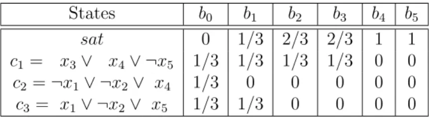
States b0 b1 b2 b3 b4 b5
sat 0 1/3 2/3 2/3 1 1
c1 = x3∨ x4∨ ¬x5 1/3 1/3 1/3 1/3 0 0
c2 =¬x1∨ ¬x2∨ x4 1/3 0 0 0 0 0
c3 = x1∨ ¬x2 ∨ x5 1/3 1/3 0 0 0 0
Table 4.1: beliefs in SAT example after taking actionsx1 =f alse,x2 =f alse, x3 =f alse, x4 =true and x5 =true.
To illustrate the POMDP reduction, we give an example in Table 4.1 for the SAT problem from Eq. 2.8 that shows how the belief is updated as we execute the sequence of actionsx1 =f alse,x2 =f alse, x3 =f alse,x4 =trueandx5 =true. Since the final belief b5 has all its mass in the state sat, we conclude that this joint assignment is satisfiable.
The POMDP obtained by our reduction has|C|+ 1 states, 2 actions, 1 observation and a planning horizon of |X|+ 1 time steps. Note that the POMDP is not stationary since the transition and reward functions are not stationary. The transition function assigns a truth value to a different variable xt+1 at each time step t while the reward function
produces a non-zero reward only at the last time step |X|. It is possible to obtain a stationary process by enlarging the state space, but this will complicate the reduction. Note also that the resulting POMDP is unobservable since the single null observation is uninformative. Unobservable POMDPs are NP-Complete [66] and therefore it makes sense that we can reduce SAT to unobservable POMDPs. The following theorem confirms that a SAT problem is satisfiable when there exists a POMDP policy with value 1.
Theorem 1. In the above reduction from SAT to POMDP, there exists a policy with value 1 iff there exists a satisfiable joint assignment.
Proof. Suppose there is a satisfiable joint assignment hx1 = a0, x2 =a1, ..., x|X| = a|X|−1i,
the transition function ensures that the final belief is b|X|(ci) = 0 ∀i and b|X|(sat) = 1
since all the clauses are satisfied. In turn, the reward function returns a value of 1 for this belief. Conversely, if we solve the POMDP and find a policy with value 1, it means that this policy selected actions that satisfied all the clauses and therefore the joint assignment corresponding to this policy is satisfiable.
Example
Lets focus on the state representation by using Eq. 2.8 as an example. Shown in column two of Table 4.1 is the initial belief state the process could be in where each clause has equal probability of being unsatisfiable. In columnsb1 tob5 is the belief state if we consider
a policy, πF that recommends the assignments¬x1 ∧x3∧ ¬x4 ∧x2∧x5. Since the belief
state has all its mass concentrated in the satisfiable state,sat, after all variables have been assigned in X, we can conclude that the original SAT problem is satisfiable and πF is an
optimal policy. An immediate reward of 1 is also gained from being in the satisfiable state. In summary, we have shown how to reformulate a SAT problem as a POMDP where the size of the state space, |C|+ 1, is linear in the number of clauses |C|.
4.2
QBF
⇒
POMDP
We now extend the SAT reduction to POMDP to work with quantified Boolean formulas (QBF) of the form
Q1x1Q2x2...Q|X|x|X| F(x1, ..., x|X|)
Without loss of generality, we require the sequence of quantifiers to be of the form ∃x1,∀x2,∃x3, ...,∀x|X|. If the sequence is non alternating, we can introduce extra quantified
variables until we satisfy our condition without changing the semantics of the formula. In the worst case, we will add |X|+ 1 new variables.
The reduction for QBF is similar to that of SAT. At each time step, the action corre-sponds to assigning a value to the next existentially quantified variable and the observation corresponds to assigning a value to the next universally quantified variable. This is be-cause the maximization over actions can be used to encode an existential quantifier and the expectation with respect to observations can be used to encode a universal quantifier. An existentially quantified variable is assigned a value by an action. We therefore relabel variables for simplicity to be xa
t and xot respectively.
We can reduce a QBF problem with alternating quantifiers to a POMDP as follows: • State space S = {sat, c1, c2, ..., c|C|}: This is the same as for SAT where state ci
indicates that the ith clause has yet to be satisfied and state sat indicates that all
clauses have been satisfied.
• Initial belief b0: We start with a uniform initial belief, i.e., b0(sat) = |C1|+1 and b0(ci) = |C1|+1 ∀i. For the QBF reduction, it is important to start with b0(sat) >0,
otherwise some observations might have 0 probability. Nevertheless, as in the SAT reduction, the precise probability of each state is not important. What matters is whether b(ci) = 0 (ci is satisfied) orb(ci)>0 (ci is not satisfied).
• Action space A={true, f alse}: Each action is an assignment of true or f alseto the lowest unassigned existentially quantified variable.
• Transition function Pr(st+1|st, at): The transition function is the same as for SAT.
When in state st =ci, the process will transition deterministically to the satisfiable
state sat if the current action satisfies clause ci. Otherwise, the process remains in
the current state.
P r(st+1|st, at) (4.4) =
1 if st =ci and at satisfies ci and st+1 =sat
1 if st =ci and at ¬satisfy ci and st+1 =ci
1 if st =st+1 =sat
0 otherwise
• Reward function R(st, at): The reward function is the same as for SAT. It returns
a non-zero reward only at the last time step where a reward of 1 is earned if the system is in the satisfiable state sat.
R(st, at) =
1 ift =|X| and st=sat
0 otherwise (4.5)
• Observation space O ={true, f alse}: Each observation is an assignment of true
or f alse to the lowest unassigned universally quantified variable.
• Observation distribution Pr(ot+1|at, st+1): The observation distribution is setup
in a way to ensure that b(ci) becomes 0 (at the next time step) when clause ci is
satisfied by the truth value assigned by the observation to the current universally quantified variable. Otherwise, b(ci) remains greater than 0 when clause ci has not
been satisfied yet. We achieve this effect by defining a deterministic observation distribution for the ci states and a stochastic observation distribution for the sat
ensure that both truth values are considered for universally quantified variables. P r(ot+1|at, st+1) (4.6) = 0 if st+1 =ci and (xot+1 :=ot+1) satisfies ci 1 if st+1 =ci and (xot+1 :=ot+1)¬satisfy ci 1
2 otherwise (i.e., st+1 =sat)
Note that the observation distribution does not depend on the current action at.
Note also that the observation probability for st+1 = sat does not have to be 1/2.
Any probability between 0 and 1 is fine.
• Horizon h=|X|/2: Two variables (one existentially quantified and one universally quantified) are processed per time step. An additional time step is created at the end for the final reward. Hence there are |X|/2 + 1 time steps (from time step 0 to time step |X|/2).
• Discount factor γ = 1: Since the process has a finite horizon, we do not use any discount factor.
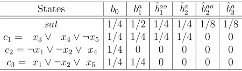
Consider again the Boolean formula in Eq. 2.8. Suppose that we quantify the 5 vari-ables as follows: ∃x1,∀x2,∃x3,∀x4,∃x5. Table4.2reports the intermediate (unnormalized)
beliefs that are obtained