A Quadratic Programming Formulation of the
Equidistant Bi-directional Loop Layout Problem
Diptesh Ghosh
W.P. No. 2015-10-05
October 2015
The main objective of the Working Paper series of IIMA is to help faculty members,research staff, and doctoral students to speedily share their research findings with professional colleagues and to test out their research findings at the pre-publication stage.
INDIAN INSTITUTE OF MANAGEMENT
AHMEDABAD – 380015
A Quadratic Programming Formulation of the
Equidistant Bi-directional Loop Layout Problem
Diptesh Ghosh
Abstract
A loop layout is a common layout used in flexible manufacturing. In such a layout, a set of stations or facilities are to be arranged in a closed loop so that the total cost of flow between each pair of facilities is minimized. The most common mathematical programming formulation of the problem is based on a quadratic assignment formulation. In this paper, we modify that formulation taking advantage of the structure of the problem.
Keywords: Flexible manufacturing, facility layout, bi-directional closed loop layout.
1
Introduction
The cost of material handling is one of the main contributors to the cost of operations in flexible manufacturing, often varying between 15 to 70% of the total cost (see, e.g., Kim and Kim, 2000). This cost depends on the efficiency with which a set of facilities (machines, stations, etc.) are assigned to candidate positions, so that a material handling agent can transfer work in progress from one facility to another. The candidate positions are arranged in a variety of ways, leading to different layout designs.
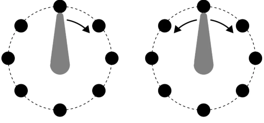
The most common is the loop layout (see Figure 1), in which the candidate positions are arranged around a closed loop. This layout is often seen when there is a radial arm which handles the inter-station flow. The radial arm can either rotate in one direction, leading to a uni-directional loop layout, or in both directions, leading to a bi-directional loop layout. The next most common layout
Figure 1: Loop layouts: Unidirectional (left) and Bi-directional (right)
is a linear layout (see Figure 2), in which positions are arranged in a line. This is common when the inter-station flow is being handled on a straight conveyor belt. There are two variants of this layout,
Figure 2: Linear layouts: Single row (left) and Double row (right)
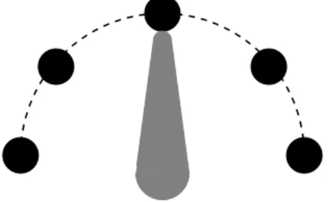
the single row facility layout, in which the positions are on one side of the belt, and the double row layout, in which the positions are on both sides of the belt. A third layout is called the semi-circular layout (see Figure 3). This is a variant of the loop layout, where the positions are arranged in a semi-circle rather than a complete loop.
Figure 3: Semi-circular layout
The loop layout problem is one of assigning facilities to positions such that the total cost of material transfer among facilities is minimized. The total cost of flow between a pair of facilities is taken as the product of the amount of flow between them and the distance between the facilities, given their positions. Formally stated the problem is the following:
The Loop Layout Problem
Given A set ofN facilities, labeled 1 throughN,N positions on the circumference of a circle, and the flowfij between facilitiesiandj for all facility pairs{i, j}.
Required An assignment of facilities to positions such that the total cost of sending flow among all pairs of facilities is minimized.
The loop layout problem is called uni-directional or bi-directional depending on how the distance between two facilities is computed. Suppose the facilities are at positionsk and l. If the distance between the positions is computed by traversing the circumference of the cycle only in the clockwise direction (or, only in the counter-clockwise direction), the problem is called the uni-directional loop layout problem. However, if the distance between the two positions is the smaller among two distances, one when traveling clockwise fromktol, and the other when traveling counter-clockwise from ktol, then the problem is called a bi-directional loop layout problem.
Several mathematical programming formulations of layout problems have been presented in the literature, although the number of formulations of the linear layout problem (both single row an double row layouts) is more than that for loop layout problems, especially in recent times. We refer an interested reader to Anjos et al. (2005), Amaral (2008), Amaral (2009), Amaral and Letchford (2012), Hungerl¨ander and Rendl (2011), etc.
Afentakis (1989) first proposed a discrete formulation for the loop layout problem. Subsequently, Kaku and Rachamadugu (1992), Kiran et al. (1992), Kiran and Karabati (1993),Bozer and Rim
(1996), Altinel and ¨Oncan (2005), and ¨Oncan and Altinel (2008) have mostly modeled the uni-directional version problem as a quadratic assignment problem. Sharp and Liu (1990) and Kiran and Karabati (1993) have proposed alternative mixed integer programming models for the problem. Saravanan and Ganesh Kumar (2013) provides an up to date review of the literature on loop layout problems.
In this paper, we provide a formulation of a special case of the bi-directional loop layout problem called the equidistant bi-directional loop layout problem (EBLLP). In this problem, each position is at equal distances from its neighboring positions. Our formulation makes use of the various symmetry conditions in the EBLLP. In Section 3, we provide an example explaining our formulation. The last section is a summary of the contribution of the paper.
2
A Mathematical Model for the EBLLP
Let the indicesl andkdenote positions from 1 throughN, and indicesiandjdenote facilities from 1 throughN occupying positions. xpq, 1≤p, q≤N are decision variables that obtain a value of 1 if facilityqoccupies positionpand 0 otherwise. The termdkl denotes the distance between positions kandl, (l > k) and is calculated as
dkl= 2πr
N ×min{(l−k),(N+k−l)} whereris the radius of the circle on which the facilities are arranged.
A mathematical programming formulation of the circular ordering problem is given below.
MODEL1: MinimizeZ = N−1 X k=1 N X l=k+1 N X i=1 N X j=1,j6=i dklfijxkixlj Subject to N X i=1 xki= 1 for 1≤k≤N (1) N X k=1 xki= 1 for 1≤i≤N (2) xki∈ {0,1} for 1≤k, i≤N.
Herez is the total “communication” cost incurred by the solution. Constraint set (2) ensures that each position has one facility assigned to it, while constraint set (1) ensures that each facility occupies only one position in the layout.
In the circular ordering problem,fij =fjifor 1≤i, j,≤N. So N X i=1 N X j=1,j6=i fijxkixlj= 2× N−1 X i=1 N X j=i+1 fijxkixlj.
Also, without loss of generality, we can specify that facility 1 occupies position 1 in the layout. If this is specified,x11 = 1, so thatP
N
k=2xk1 =P
N
follows. MODEL2: MinimizeZ= N X l=2 N X j=2 d1lf1jxlj+ 2 N−1 X k=2 N X l=k+1 N−1 X i=2 N X j=i+1 dklfijxkixlj Subject to N X i=2 xki= 1 for 2≤k≤N (3) N X k=2 xki= 1 for 2≤i≤N (4) xki∈ {0,1} for 2≤k, i≤N.
Constraint set (3) can next be used to modify the model and reduce the number of variables. For eachk, 2≤k≤N, xkN = 1− N−1 X i=2 xki. (5)
So, this removesN−1 variables from the formulation. However, the constraints that xkN ∈ {0,1}
gets modified to constraints of the form N−1
X
i=2
xki≤1 for eachk= 2, . . . , N. (6)
In a similar fashion, from constraint set (4) we see that for eachi, 2≤i≤N,
xN i= 1− N−1
X
k=2
xki, (7)
and the restriction onxN i to be binary yields constraints of the form N−1
X
k=2
xki≤1 for eachi= 2, . . . , N. (8)
Also, since at most one amongx52throughx5(n−1)can acquire a value of 1 in any feasible solution,
we have N−1 X k=2 N−1 X i=2 xk1≥N−3. (9)
The objective function in MODEL2 can be written asZ =Z1+2ZrwhereZ1=PNl=2PNj=2d1lf1jxlj is the cost of communication between facility 1 (located at position 1) with the other facilities, and 2Zr= 2PN−1 k=2 PN l=k+1 PN−1 i=2 PN
j=i+1dklfijxkixljis the cost of communication between all facilities
NowZ1= N X l=2 N X j=2 d1lf1jxlj = N X l=2 d1l (N−1 X j=2 f1jxlj+f1NxlN ) = N X l=2 d1l ( f1N + N−1 X j=2 (f1j−f1N)xlj ) (using eqn (5)) = N X l=2 d1lf1N + N X l=2 d1l N−1 X j=2 (f1j−f1N)xlj = N X l=2 d1lf1N + N−1 X l=2 d1l N−1 X j=2 (f1j−f1N)xlj+d1N N−1 X j=2 (f1j−f1N)xN j = N X l=2 d1lf1N + N−1 X l=2 d1l N−1 X j=2 (f1j−f1N)xlj+ d1N N−1 X j=2 (f1j−f1N) 1− N−1 X l=2 xlj ! (using eqn (7)) = N X l=2 d1lf1N +d1N N−1 X j=2 (f1j−f1N) + N−1 X l=2 d1l N−1 X j=2 (f1j−f1N)xlj−d1N N−1 X j=2 (f1j−f1N) N−1 X l=2 xlj = N X l=2 d1lf1N +d1N N−1 X j=2 (f1j−f1N) + N−1 X j=2 N−1 X l=2 (d1l−d1N)(f1j−f1N)xlj. (10)
Note thatd1p =d1(N+1−p) for all i, 2≤i ≤N/2. So the coefficients of xpj and x(N+1−p)j in the expansion ofPN
l=2
PN
j=2d1lf1jxlj will be identical for allp, 2≤p≤N/2. So when equation (7) is
applied to obtain expression (10) forZ1, the expression will not include termsx2,j,j= 2, . . . , N−1.
SimilarlyZr= N−1 X k=2 N X l=k+1 N−1 X i=2 N X j=i+1 dklfijxkixlj = N−1 X k=2 N X l=k+1 dkl N−1 X i=2 ( N−1 X j=i+1 fijxkixlj+fiNxkixlN ) = N−1 X k=2 N X l=k+1 dkl N−1 X i=2 ( N−1 X j=i+1
fijxkixlj+fiNxki1− N−1 X j=2 xlj ) (using eqn (5)) = N−1 X k=2 N X l=k+1 dkl N−1 X i=2 fiNxki+ N−1 X k=2 N X l=k+1 dkl N−1 X i=2 N−1 X j=i+1 (fij−fiN)xkixlj = N−1 X k=2 N−1 X i=2 N X l=k+1 dklfiNxki+ N−1 X k=2 N−1 X i=2 N−1 X j=i+1 ( N−1 X l=k+1
dkl(fij−fiN)xkixlj+
dkN(fij−fiN)xkixN j
= N−1 X k=2 N−1 X i=2 N X l=k+1 dklfiNxki+ N−1 X k=2 N−1 X i=2 N−1 X j=i+1 ( N−1 X l=k+1
dkl(fij−fiN)xkixlj+
dkN(fij−fiN)xki 1− k X l=2 xlj− N−1 X l=k+1 xlj !) (using eqn (7)) = N−1 X k=2 N−1 X i=2 N X l=k+1 fiNdklxki+ N−1 X k=2 N−1 X i=2 N−1 X j=i+1
dkN(fij−fiN)xki+ N−1 X k=2 N−1 X i=2 N−1 X j=i+1 N−1 X l=k+1
(dkl−dkN)(fij−fiN)xkixlj− N−1 X k=2 N−1 X i=2 N−1 X j=i+1 k X l=2
dkN(fij−fiN)xkixlj. (11)
Using expressions (10) and (11) for Z1 and Zr respectively, the cost function Z for the circular
ordering problem can be written as Z=Z1+ 2Zr = N X l=2 d1lf1N+ N−1 X j=2 d1N(f1j−f1N) + N−1 X j=2 N−1 X l=2 (d1l−d1N)(f1j−f1N)xlj+ 2 N−1 X k=2 N−1 X i=2 N X l=k+1 fiNdklxki+ 2 N−1 X k=2 N−1 X i=2 N−1 X j=i+1
dkN(fij−fiN)xki+
2 N−1 X k=2 N−1 X i=2 N−1 X j=i+1 N−1 X l=k+1 (dkl−dkN)(fij−fiN)xkixlj−2 N−1 X k=2 N−1 X i=2 N−1 X j=i+1 k X l=2 dkN(fij−fiN)xkixlj.
Since the termsPN
l=2d1lf1N andd1NP N−1
j=2 (f1j−f1N) are independent ofxki values, the circular ordering problem is the problem of minimizing the following non-linear function subject to the constraint sets (6) and (8).
Z= N−1 X j=2 N−1 X l=2 (d1l−d1N)(f1j−f1N)xlj+ 2 N−1 X k=2 N−1 X i=2 N X l=k+1 fiNdklxki+ 2 N−1 X k=2 N−1 X i=2 N−1 X j=i+1 dkN(fij−fiN)xki+ 2 N−1 X k=2 N−1 X i=2 N−1 X j=i+1 N−1 X l=k+1
(dkl−dkN)(fij−fiN)xkixlj−2 N−1 X k=2 N−1 X i=2 N−1 X j=i+1 k X l=2
dkN(fij−fiN)xkixlj. (12)
3
An Example
Consider an instance of circular ordering in which we have to order five facilities around a circle. The frequency of communication between pairs of facilities is given in the table below.
F= [fij] 1 2 3 4 5 1 - 5 2 7 8 2 5 - 6 4 3 3 2 6 - 9 1 4 7 4 9 - 7 5 8 3 1 7
-Without loss of generality, we assume that the radius of the circle is 5/2πunits so that the distance between consecutive positions is 1 unit. We also assume that facility 1 is located at position 1 (as specified in MODEL2).
In this example, the term Z1 when evaluated without making use of equations (5) and (7) is
given by Z1= 5x22+ 2x23+ 7x24+ ‘ 8x25+ 10x32+ 4x33+ 14x34+ 16x35+ 10x42+ 4x43+ 14x44+ 16x45+ 5x52+ 2x53+ 7x54+ 8x55. From (5)x25= 1−(x22+x23+x24);x35= 1−(x32+x33+x34);x45= 1−(x42+x43+x44); and
x55= 1−(x52+x53+x54). Substituting these terms,
Z1= 48−3x22−6x23−x24−6x32−12x33−2x34−6x42−12x43−2x44−3x52−6x53−x54.
Next from (7)x52= 1−(x22+x32+x42);x53= 1−(x23+x33+x43); andx54= 1−(x24+x34+x44).
Substituting these terms,
Z1= 38−3x32−6x33−x34−3x42−6x43−x44; (13)
corresponding to expression (10).
The termZr when evaluated without making use of equations (5) and (7) is given by
Zr=6x22x33+ 4x22x34+ 3x22x35+ 9x23x34+ 1x23x35+ 7x24x35+ 12x22x43+ 8x22x44+ 6x22x45+ 18x23x44+ 2x23x45+ 14x24x45+ 12x22x53+ 8x22x54+ 6x22x55+ 18x23x54+ 2x23x55+ 14x24x55+ 6x32x43+ 4x32x44+ 3x32x45+ 9x33x44+ 1x33x45+ 7x34x45+ 12x32x53+ 8x32x54+ 6x32x55+ 18x33x54+ 2x33x55+ 14x34x55+ 6x42x53+ 4x42x54+ 3x42x55+ 9x43x54+ 1x43x55+ 7x44x55.
Using equations (5) to eliminatex35,x45, andx55, we have
Zr=15x22+ 5x23+ 35x24+ 9x32+ 3x33+ 21x34+ 3x42+x43+ 7x44+ 3x22x33+x22x34+ 8x23x34+ 6x22x43+ 2x22x44+ 16x23x44+ 6x22x53+ 2x22x54+ 16x23x54+ 3x32x43+x32x44+ 8x33x44+ 6x32x53+ 2x32x54+ 16x33x54+ 3x42x53+ x42x54+ 8x43x54−3x22x32−7x24x32−7x24x33−7x24x34−6x22x42−2x23x42− 2x23x43−14x24x42−14x24x43−14x24x44−6x22x52−2x23x52−2x23x53−14x24x52− 14x24x53−14x24x54−3x32x42−7x34x42−7x34x43−7x34x44−6x32x52−2x33x52− 2x33x53−14x34x52−14x34x53−14x34x54−3x42x52−7x44x52−7x44x53−7x44x54− x23x32−x23x33−x33x42−x33x43−x43x52−x43x53.
Next using equations (7) to eliminatex52,x53, andx54, and noting that for any binary variabley,
y2=y, we get Zr=23x22+ 19x23+ 7x24+ 17x32+ 17x33−7x34+ 7x42+ 8x43−7x44− x22x33+ 13x22x34+ 6x23x34+x22x43+ 7x22x44+ 7x23x44−2x32x43+ 6x32x44−x33x44+ 9x22x32+ 5x24x32−9x24x33+ 21x24x34+ 3x22x42−3x23x42+x23x43−x24x42−8x24x43+ 7x24x44+ 6x32x42+ 6x34x42−x34x43+ 14x34x44−5x23x32+ 3x23x33−2x33x42+ 2x33x43+ 6x44x42−x44x43−2x43x42−4x22x23+ 12x22x24−2x23x24−4x33x32+ 12x34x32−2x34x33.
This corresponds to expression (11).
So the cost function for the instance is given by Z=Z1+ 2Zr =38 + 46x22+ 38x23+ 14x24+ 31x32+ 28x33−15x34+ 11x42+ 10x43−15x44− =2x22x33+ 26x22x34+ 12x23x34+ 2x22x43+ 14x22x44+ 14x23x44−4x32x43+ 12x32x44−2x33x44+ =18x22x32+ 10x24x32−18x24x33+ 42x24x34+ 6x22x42−6x23x42+ 2x23x43−2x24x42−16x24x43+ =14x24x44+ 12x32x42+ 12x34x42−2x34x43+ 28x34x44−10x23x32+ 6x23x33−4x33x42+ 4x33x43+ =12x44x42−2x44x43−4x43x42−8x22x23+ 24x22x24−4x23x24−8x33x32+ 24x34x32−4x34x33;
and the solution to the instance will be the minimizer of this function subject to the constraints
4 X i=2 xki≤1 for eachk= 2, . . . ,4; 4 X k=2 xki≤1 for eachi= 2, . . . ,4; 4 X k=2 4 X i=2 xk1≥2;
and the condition that allxij variables are binary variables.
4
Summary
In this paper we formulated a bi-directional loop layout problem with equidistant facilities as a quadratic programming problem. Using the quadratic assignment problem as a base, we use the symmetry properties of the problem to simplify the cost function. We also convert the constraints of the problem from the more restrictive equality constraints to the less restrictive inequality con-straints. We provide an example of our formulation on a problem with five facilities and five candidate locations.
The formulation presented here is amenable to the use of preprocessing rules and solution through branch and bound procedures. These will be interesting directions for further research on this problem.
References
Afentakis, P. (1989). A loop layout design problem for flexible manufacturing systems. The Inter-national Journal of Flexible Manufacturing Systems, 1:175–196.
Altinel, I. K. and ¨Oncan, T. (2005). Design of unidirectional cyclic layouts. International Journal of Production Research, 43(19):3893–4008.
Amaral, A. R. S. (2008). An Exact Approach to the One-Dimensional Facility Layout Problem.
Operations Research, 56(4):1026–1033.
Amaral, A. R. S. (2009). A mixed 0-1 linear programming formulation for the exact solution of the minimum linear arrangement problem. Optimization Letters, 3:513–520.
Amaral, A. R. S. and Letchford, A. N. (2012). A polyhedral approach to the single row facil-ity layout problem. Mathematical Programming. Available at http://dx.doi.org/10.1007/ s10107-012-0533-z.
Anjos, M. F., Kennings, A., and Vannelli, A. (2005). A semidefinite optimization approach for the single-row layout problem with unequal dimensions. Discrete Optimization, 2(2):113–122. Bozer, Y. A. and Rim, S.-C. (1996). A branch and bound method for solving the bidirectional
circular layout problem. Applied Mathematical Modelling, 20:342–351.
Hungerl¨ander, P. and Rendl, F. (2011). Semidefinite relaxations of ordering problems. Mathematical Programming B.
Kaku, B. and Rachamadugu, R. (1992). Layout design for flexible manufacturing systems.European Journal Of Operational Research, 57(2):224–230.
Kim, J.-G. and Kim, Y.-D. (2000). Layout planning for facilities with fixed shapes and input and output points. International Journal of Production Research, 38(18):4635–4653.
Kiran, A. and Karabati, S. (1993). Exact and approximate algorithms for the loop layout problem.
Production Planning and Control, 4:253–259.
Kiran, A., ¨Unal, A., and Karabati, S. (1992). A location problem on unicyclic networks: Balanced case. European Journal Of Operational Research, 62:194–202.
¨
Oncan, T. and Altinel, I. K. (2008). Exact solution procedures for the balanced unidirectional cyclic layout problem. European Journal Of Operational Research, 189:609–623.
Saravanan, M. and Ganesh Kumar, S. (2013). Different approaches for the loop layout problems: a review. International Journal of Advanced Manufacturing Technology, 69:2513–2529.
Sharp, G. and Liu, F. (1990). An analytical method for configuring fixed path closed loop material handling systems. International Journal of Production Research, 28(4):757–783.