Stochastic functional descent for learning Support Vector Machines

OpenBU http://open.bu.edu

Theses & Dissertations Boston University Theses & Dissertations

2014

Stochastic functional descent for

learning Support Vector Machines

https://hdl.handle.net/2144/14104

GRADUATE SCHOOL OF ARTS AND SCIENCES

Thesis

STOCHASTIC FUNCTIONAL DESCENT FOR

LEARNING SUPPORT VECTOR MACHINES

by

KUN HE

B.Eng., Zhejiang University, 2010

Submitted in partial fulfillment of the

requirements for the degree of

Master of Science

2014

LEARNING SUPPORT VECTOR MACHINES

KUN HE

ABSTRACT

We present a novel method for learning Support Vector Machines (SVMs) in the online setting. Our method is generally applicable in that it handles the online learning of the binary, multiclass, and structural SVMs in a unified view.

The SVM learning problem consists of optimizing a convex objective function that is composed of two parts: the hinge loss and quadratic (L2) regularization. To date,

the predominant family of approaches for online SVM learning has been gradient-based methods, such as Stochastic Gradient Descent (SGD). Unfortunately, we note that there are two drawbacks in such approaches: first, gradient-based methods are based on a local linear approximation to the function being optimized, but since the hinge loss is piecewise-linear and nonsmooth, this approximation can be ill-behaved. Second, existing online SVM learning approaches share the same problem formu-lation with batch SVM learning methods, and they all need to tune a fixed global

regularization parameter by cross validation. On the one hand, global regularization is ineffective in handling local irregularities encountered in the online setting; on the other hand, even though the learning problem for a particular global regularization parameter value may be efficiently solved, repeatedly solving for a wide range of values can be costly.

We intend to tackle these two problems with our approach. To address the first problem, we propose to perform implicit online update steps to optimize the hinge loss, as opposed to explicit (or gradient-based) updates that utilize subgradients to perform local linearization. Regarding the second problem, we propose to enforce

having a fixed global regularization term.

Our theoretical analysis suggests that our classifier update steps progressively optimize the structured hinge loss, with the rate controlled by a sequence of regular-ization parameters; setting these parameters is analogous to setting the stepsizes in gradient-based methods. In addition, we give sufficient conditions for the algorithm’s convergence. Experimentally, our online algorithm can match optimal classification performances given by other state-of-the-art online SVM learning methods, as well as batch learning methods, after only one or two passes over the training data. More importantly, our algorithm can attain these results without doing cross validation, while all other methods must perform time-consuming cross validation to determine the optimal choice of the global regularization parameter.

1 Introduction 1

1.1 Background . . . 4

1.2 Review of structural SVM learning . . . 6

1.3 Main ideas of proposed method . . . 14

1.4 Outline of thesis . . . 17

2 Related Work 18 2.1 Online methods for SVM learning . . . 18

2.2 Regularization in online learning . . . 21

2.3 Boosting and functional gradient descent . . . 22

3 Proposed Approach 24 3.1 Derivation . . . 24

3.2 Algorithmic details . . . 28

3.3 Implementation details and practical considerations . . . 31

3.4 Special cases . . . 33

3.5 Concluding remarks . . . 34

4 Theoretical Analysis 36 4.1 Effect of local L2 regularization . . . 36

4.2 Sufficient condition for convergence . . . 40

4.3 Concluding remarks . . . 41

5.1 Binary classification . . . 43

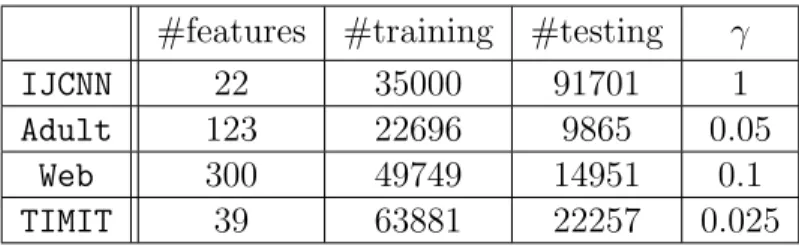
5.1.1 Experimental setup . . . 44

5.1.2 Parameter studies . . . 45

5.1.3 Comparisons with other SVM learning methods . . . 50

5.2 Object localization: TU Darmstadt cows and Caltech faces . . . 59

5.2.1 Formulation . . . 59

5.2.2 Experimental setup . . . 60

5.2.3 Results . . . 61

5.3 Object detection: PASCAL VOC 2007 . . . 63

5.3.1 Experimental setup . . . 65

5.3.2 Results and analysis . . . 69

5.4 Concluding remarks . . . 76

6 Conclusion and Future Work 77

References 82

5.1 Summary of binary datasets. . . 45 5.2 Binary classification: optimal regularization parameter values λOP T . 51

5.3 Test errors after two epochs on four binary datasets, resulting from 5 randomized runs. . . 54 5.4 Binary classification: number of kernel evaluations required by each

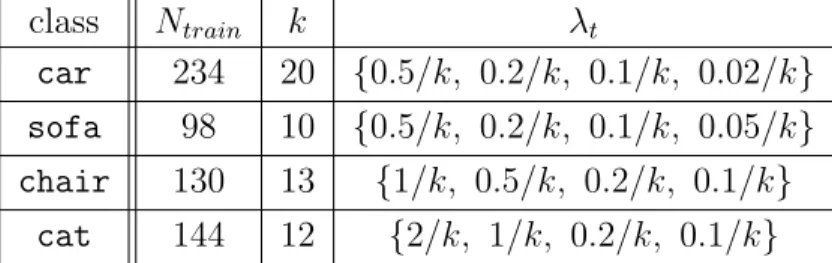
algorithm . . . 55 5.5 Algorithm parameters for PASCAL VOC 2007 experiments. . . 66

1·1 Examples of structured output prediction problems . . . 5

3·1 Illustration of the regularized classifier update steps . . . 27

5·1 Parameter study on the size of training subsets . . . 47

5·2 Parameter study on the regularization parameterλt . . . 49

5·3 Comparison of binary SVM learning algorithms on four datasets, against number of examples processed . . . 53

5·4 Comparison of binary SVM learning algorithms on four datasets, against number of support vectors . . . 56

5·5 Sample cow and face localization results . . . 63

5·6 Overlap-recall curves for PASCAL VOC 2007car class . . . 70

5·7 Overlap-recall curves for PASCAL VOC 2007sofa class . . . 71

5·8 Overlap-recall curves for PASCAL VOC 2007chair class . . . 72

5·9 Overlap-recall curves for PASCAL VOC 2007cat class . . . 73

ACM . . . Association for Computing Machinery AUC . . . Area Under Curve

HOG . . . Histogram of Oriented Gradients

IEEE . . . Institute of Electrical and Electronics Engineers KKT . . . Karush-Kuhn-Tucker (optimality conditions) QP . . . Quadratic Program

RBF . . . Radial Basis Function

RKHS . . . Reproducing Kernel Hilbert Space SGD . . . Stochastic Gradient Descent SIFT . . . Scale-Invariant Feature Transform SVM . . . Support Vector Machine

Chapter 1

Introduction

In this thesis, we are concerned with the problem of learning Support Vector Machines (SVMs) in an online setting. We present a novel online SVM learning algorithm, and demonstrate both theoretically and empirically that it has desirable properties.

The SVM is a powerful tool to solve classification, regression, and ranking prob-lems, especially when equipped with nonlinear kernels. Its generalization, the struc-tural SVM, is one of the most widely-used methods for solving structured output prediction problems. However, due to the relatively high complexity in learning, the application of SVM in large-scale settings has been limited, since it is often infeasible or difficult to learn the classifier all at once with large training data. One way to im-prove the efficiency of SVM learning is to use online approaches, where the classifier is learned incrementally by a series of classifier updates computed using streaming data or random training subsets step by step. We focus on the online setting in this thesis.

Currently, the most prominent family of online learning methods for (structural) SVMs are gradient-based methods. For example, a well-known method in this family is Stochastic Gradient Descent (SGD), a standard online optimization technique that uses random subsets to estimate gradients1 of the learning objective and performs

1_{For SVM learning, the actual algorithm is usually stochasticsubgradientdescent since the SVM}

objective is nonsmooth. However, following common convention, we still refer to the algorithm as “gradient descent”.

gradient descent. When applied to SVM learning, gradient-based methods, as well as other online methods, share the same problem formulation with offline, or “batch” learning methods that utilize the entire training set altogether. However, with careful application of online optimization techniques, state-the-art online methods can of-ten achieve similar SVM learning results with batch methods, while being significantly faster.

Unfortunately, we note that existing online SVM learning methods still have draw-backs in two aspects. The first drawback specifically applies to gradient-based meth-ods. In gradient-based methods, the fundamental idea is to perform a local first-order approximation, or linearization, of the function being optimized using its gradients or subgradients. However, as is often the case with curved functions, this local lin-earization often can overestimate the decrease in function values and lead to gradient steps that are ill-behaved. Although various fixes to gradient methods exist, it is often observed that tuning them can be complicated and time-consuming.

The second drawback applies generally to existing online SVM learning methods. The SVM objective function is composed of two terms: the hinge loss and a quadratic (L2) regularization term. The regularization term isglobal in the sense that it applies

to the entire classifier being learned, and it has proved to be effective in the batch setting. However, we argue that global regularization is ineffective in handling local

irregularities encountered in the online setting, where data can arrive out of order and exhibit high variance. Moreover, having a fixed global regularization term means that its weighting parameter needs to be tuned using cross validation, an operation that is often costly.

This thesis is motivated to deal with the two problems mentioned above. Inspired by recent advances in online learning, we propose to performimplicit online updates that more faithfully follow the objective function, rather than explicit updates that

utilize (sub)gradients. Such an idea has not been widely applied in SVM learning. Moreover, to handle local irregularities in the online setting, we follow a more estab-lished idea of performing local regularization during classifier updates, while removing the global regularization term.

The benefits of our approach are twofold: first, by performing implicit updates and regularizing each update step, our method can faithfully and steadily optimize the hinge loss in an online fashion, resulting in fast convergence and good generalization performance. Secondly, we theoretically justify that our local regularization term can be interpreted as a stepsize control operation; therefore, we can adopt standard step-size techniques that ensure good convergence rates. In contrast, in traditional SVM learning, although heuristics and rules of thumb exist for setting the regularization pa-rameter, theoretical guidelines are still lacking and cross validation is often inevitable for deciding the parameter value that gives optimal generalization performance.

We evaluate the performance of our method on two types of real-world structured prediction problems. In the fist set of experiments, we focus on binary classification, which can be seen as a special case of structured prediction. We experimentally com-pare our approach to several state-of-the-art online binary SVM learning approaches on four standard datasets. The results show that our online method, using only local information in the random training subsets, is significantly more stable than gradient-based methods such as SGD. Moreover, our method gives comparable performance to other methods having access to the entire training set. In the second set of exper-iments, we proceed to the more complicated structured prediction problem of visual object localization/detection, in order to verify that our method also applies to this generalized case. There, we demonstrate that our online method can usually achieve comparable results with batch learning methods, after only one or two sequential passes over the training set. It is important to emphasize that all of our results are

obtained without setting the regularization parameter using cross validation, while this operation is a must for all competing methods.

To summarize, our contribution is a novel online method for learning structural SVMs that has the following features:

• it enjoys theoretical convergence guarantees under mild conditions;

• it has a principled interpretation of the regularization parameter and thus can set it in principled ways;

• empirically, its performance can match or approach those given by state-of-the-art batch or online SVM learning methods, without performing cross validation. We first review necessary technical details in the remainder of this chapter before developing and evaluating our approach in later chapters. Section 1.1 introduces readers to structured output prediction. Section 1.2 reviews the basic structural SVM formulation. Then, we briefly motivate and summarize the main ideas behind our approach in Section 1.3. An outline of the thesis will be given at the end of this chapter.

1.1

Background

In this section, we would like to motivate the use of SVMs to solve real-world problems. We prefer to state our motivations by introducing the general structured output prediction problems, since this class of problems subsumes the better known binary and multiclass prediction problems. Stated differently, the structural SVM, designed to solve structured output prediction problems, also reduces to the classical binary and multiclass SVMs as special cases. We introduce structured output prediction in this section and formally show how it reduces to binary and multiclass classification in the next section.

Figure 1·1: Examples of structured output prediction problems: ob-ject detection, human pose estimation, and natural language parsing. Images are taken from the PASCAL VOC 2007 challenge (Evering-ham et al., 2010), (Tian and Sclaroff, 2010), and (Tsochantaridis et al., 2006), respectively.

The problem of structured output prediction is a problem where given an input pattern, the desired prediction output is astructured object, such as sequences, trees, strings, or graphs. Such problems naturally occur in many application domains, such as computer vision and natural language processing. We present some concrete examples in Figure 1·1. The first example is object localization: given an input im-age (taken from the training set of PASCAL VOC 2007 challenge (Everingham et al., 2010)), the task is to find an object of interest, represented by a bounding box around its location. Here the output is a four-dimensional vector(left,right,top,bottom) indi-cating the location of the bounding box in image coordinates. The second example is human pose estimation (Tian and Sclaroff, 2010), which can be regarded as a general-ized object detection problem: instead of producing one bounding box for the human body, the task is to output the location, orientation and scale for each one of the body parts. Lastly, there is an example from the natural language processing domain (Tsochantaridis et al., 2006), where the task is to output a parse tree corresponding to an input sentence.

prop-erties:

• The output label is multi-dimensional, which means that the decision problem is not a binary (yes/no style) problem. Making a prediction (i.e. doing inference) is more complicated.

• There is correlation or interaction between the output dimensions. For example, the right edge of the bounding box should have a greater image coordinate than the left edge. This makes predicting each dimension separately suboptimal, and it is more desirable to search for the best combinatorial configuration.

• The number of possible labels, or the size of the output space, is large. Usually, it is exponential in the number of dimensions, and this renders brute-force examination of all labels ineffective.

Given these properties, to successfully learn the complex input-output interac-tions, it is usually necessary to have training sets of medium to large sizes.

The basic machinery we will consider in this thesis is the structural SVM (Tsochan-taridis et al., 2006), a generalization of the binary SVM to handle structured outputs. It has largely been the method of choice for solving structured prediction problems. In the next section, we will review essential details of the structural SVM, and show that it is a natural generalization of the classical SVM by outlining the reductions.

1.2

Review of structural SVM learning

In this section, we intend to give a brief review of the structural SVM learning prob-lem, in order to make this thesis self-contained. As mentioned in the previous section, we prefer to work with the more general structural SVM formulation, since it reduces to the binary and multiclass SVMs as special cases. Our review is inspired by seminal

works on this topic such as (Tsochantaridis et al., 2006) and (Joachims et al., 2009), and interested readers are referred to them for more in-depth details and analysis.

Let us consider a supervised learning setting with training set {(xi, yi)|i ∈ S},

where examples xi are from input space X, labels yi belong to output space Y,

and S = {1, . . . , n}. We emphasize that Y can consist of structured objects such as strings, graphs, and trees. We are mainly interested in structured classification,

i.e. Y is discrete. Our goal is to learn a discriminant function f(x, y) such that the label y assigned to x is the one that maximizes f(x, y). It is also called a

compatibility function as the function value can be regarded as a measure of com-patibility between the example x and its assigned label y. Obviously, we hope that

yi = argmaxy∈Yf(xi, y),∀i ∈ S. When that is not possible, i.e. the data is not

perfectly separable, we will suffer some loss.

In this thesis, we assume that the discriminant function, or more briefly the clas-sifier, can be parameterized in a linear form as f(x, y) = wT_{Ψ(x, y), with w being}

a parameter vector, and Ψ(x, y) being an appropriately designed joint feature map. With a little abuse of notation, we will refer to w, the classifier’s parameter vector, as the classifier from now on.

Above, we used the linear inner product, or the linear kernel, in the parameteri-zation of f. More generally, f can be parameterized differently to permit the use of inner products in reproducing kernel Hilbert spaces (RKHS), commonly referred to as nonlinear kernels. An RKHS, denoted by H, is an inner product space in which the inner product hΨ(x, y),Ψ(x0, y0)i is evaluated through the joint kernel function K((x, y),(x0, y0)). In this case, the joint feature map Ψ(x, y) is said to be induced

by K, and often cannot be explicitly constructed (for example, it can be of infinite dimensionality). To embed f in a general RKHS, we write f(x, y) =hw,Ψ(x, y)i to indicate that the corresponding inner product h·,·i is employed. This is a implicit

linear parameterization of f, since it is possible that the parameter vector w can no longer be explicitly constructed. Throughout this thesis, we use the more general im-plicit linear parameterization, in order to make sure that our formulation also handles general kernel classifiers.

Now we are ready to discuss the details of the structural SVM. The structural SVM, proposed by (Tsochantaridis et al., 2006), offers a “large-margin” solution to the problem of learning f, or more precisely w. In (Tsochantaridis et al., 2006), two formulations are presented: margin rescaling and slack rescaling. In this thesis, we study the more widely-used margin rescaling case, corresponding to the optimization problem labeled SVM∆m

1 in (Tsochantaridis et al., 2006):

Optimization Problem (OP) 1. (structural SVM primal)

min w,ξ λ 2||w|| 2 H+ 1 n n X i=1 ξi (1.1) s.t. hw, δΨi(y)i ≥∆(yi, y)−ξi, ∀i∈S,∀y∈ Y (1.2)

In this formulation, we use the shorthand δΨi(y) = Ψ(xi, yi)−Ψ(xi, y). Slack

variables ξi are added to account for the non-separable case, and their average is the

amount of loss that we suffer from misclassification. λ is a parameter controlling the trade-off between the strengths of loss minimization and regularization. We will refer toλ as theregularization parameter from now on.

In structural SVM, it is important to define a proper loss function ∆(yi, y) to

encode the penalty of misclassifying yi into y. A simple example of such a function

is the 0-1 loss: ∆(yi, y) = 1[yi 6= y], but it is usually considered simplistic. In

a sense, ∆(yi, y) encodes the structure of the problem at hand, since it is able to

penalize different structured labels y differently according to their similarity withyi.

reasonable choice for ∆. As noted in (Tsochantaridis et al., 2006), to ensure well-defined algorithm behavior and permit certain theoretical guarantees, ∆(yi, y) should

be nonnegative, achieve zero only when y=yi, and be upper-bounded.

We refer to the formulation presented in OP1 as the “margin maximization” view of structural SVM learning. The constraint Eq.(1.2) enforces a certain mar-gin between the ground truth score hw,Ψ(xi, yi)i and the score of a wrong label

hw,Ψ(xi, y)i, for ∀i∈S.

On the other hand, in order to facilitate the development of our approach later, we would like to point out that the structural SVM learning problem can be viewed from the general machine learning perspective of loss minimization and regularization. To show that, let us first define the structured hinge loss with respect to the training set

S as H(w, S)=∆ 1 n n X i=1 max y∈Y [∆(yi, y)− hw, δΨi(y)i]. (1.3)

Then, we can show that OP1 is equivalent to the following unconstrained problem using basic optimization arguments:

min w λ 2||w|| 2 H+H(w, S). (1.4)

To see that, note that OP1 is a minimization problem; therefore, at optimality the optimal slack variablesξ_i∗ should make the constraints Eq.(1.2) tight,i.e.

ξ_i∗ = max

y∈Y [∆(yi, y)− hw, δΨi(y)i],∀i∈S. (1.5)

Replacing the slack variables with this equation gives the unconstrained problem in Eq.(1.4). This formulation bears the usual interpretation of regularized loss

min-imization: we seek a classifier w to minimize the structured hinge loss as defined in Eq.(1.3), and in order to prevent overfitting, we add an L2 regularizer λ₂||w||2H

and try to balance the weighting between loss minimization and regularization. The regularization parameter λ usually needs to be hand-tuned or determined by cross validation.

Recall that we parameterize the classifierf by a parameter vectorwin an RKHS. By now, we have formulated the learning problem but have not shown how to obtain w. Fortunately, the next theorem provides a canonical form of classifiers learned by solving regularized loss minimization problems in an RKHS, including the structural SVM problem that we study here. This theorem, described in (Hofmann et al., 2008), is a generalized version of the classical Representer Theorem (Kimeldorf and Wahba, 1970), and it essentially states that the classifier resulting from solving a problem like Eq.(1.4) is a weighted sum of kernel evaluations between the input feature and all the training examples.

Theorem 1. A generalized Representer Theorem (Corollary 13 in (Hofmann et al., 2008))

Denote by H an RKHS on X × Y with kernel K and let S = {(xi, yi)}ni=1.

Fur-thermore, let C(f, S)be a loss functional, andΩbe a strictly monotonically increasing function. Then for the regularized loss minimization problem

f∗ = argmin

f∈H

C(f, S) + Ω(||f||2_H), (1.6)

the solution admits the form of

f∗(·) = n X i=1 X y∈Y αy_iK(·,(xi, y)). (1.7)

Now let us interpret the implications of this theorem. If we take C to be the structured hinge loss, and set Ω to be 1₂I, where I is the identity function, then we recover the structural SVM formulation in OP1. So now we can be certain that the SVM classifier we seek should have the form of Eq.(1.7).

Furthermore, it is also proved in (Hofmann et al., 2008), Proposition 14 that for the special case of structural SVM, the coefficientsαare the solutions to the following quadratic program (QP):

Optimization Problem (OP) 2. (Structural SVM dual)

max α − 1 2 X i,j∈S X y,y0_∈Y α_iyαy_j0K˜(i, y, j, y0) +X i∈S X y∈Y ∆(yi, y)αyi (1.8) s.t. X y∈Y αy_i = 1 nλ, ∀i∈S (1.9) αy_i ≥0, ∀i∈S, ∀y ∈ Y (1.10)

Note that in order to simplify notation, we write ˜K(i, y, j, y0) = hδΨi(y), δΨj(y0)i=

K((xi, yi),(xj, yj))−K((xi, yi),(xj, y0))−K((xi, y),(xj, yj))+K((xi, y),(xj, y0)) in the

above formulation. The solution to this dual problem then gives the kernelized form of f, in accordance with Eq.(1.7):

f(x, y) = hw,Ψ(x, y)i= X

i∈S,¯y∈Y

αy_i¯[K((xi, yi),(x, y))−K((xi,y¯),(x, y))]. (1.11)

In fact, OP2 is the Wolfe dual of OP1, and every αy_i in OP2 is a dual variable. By dualizing OP1, we convert the problem of finding the (primal) parameter vector w into finding the dual solution vector α. The dual problem is not only easier to solve (it has simple box constraints as opposed to complex primal constraints Eq.(1.2)), but is also the only accessible formulation when the kernelK(·,·) is nonlinear.

In the above derivation, we have applied a generalized Representer Theorem de-scribed in (Hofmann et al., 2008). This theorem is tailored for structured prediction, and is different from the the classical Representer Theorem described in (Kimeldorf and Wahba, 1970), which only considers the case where the RKHS is defined on X

but notX × Y.

Binary case

As noted earlier, the classical binary SVM is a special case of structural SVM. In the binary case, the formulation is simplified by adopting the following specialized loss function and joint feature map:

∆(yi, y) = 1[yi 6=y], (1.12)

Ψ(x, y) = 1

2yψ(x). (1.13) If we plug these definitions into the structural SVM formulation (OP1), then we get the following simplified problem:

min w,ξ λ 2||w|| 2 H+ 1 n n X i=1 ξi (1.14) s.t. yihw, ψ(xi)i ≥1−ξi, ∀i∈S, (1.15)

which is the same as the binary SVM2_{. Conversely, we can clearly see from Eq.(1.12)}

and Eq.(1.13) that the structural SVM generalizes the binary SVM in at least two aspects: the loss function and the feature map.

2_{Strictly speaking, the binary SVM often assumes an additional bias termbso that the classifier}

ishw, ψ(x)i+b. To ensure consistency with the structural SVM formulation, we omit the bias term

here but note that it can be implicitly handled, for example in the linear case, by adding a constant

Multiclass case

We note that the reduction from the structural SVM to the 1-vs-all multiclass SVM (Crammer and Singer, 2002) has been described in (Tsochantaridis et al., 2006), and therefore refer readers to that paper for a more general and complete treatment of this topic. Instead, here we intend to summarize and interpret the key steps in the reduction, bearing minor notational differences from (Tsochantaridis et al., 2006).

In the multiclass case, we assume that there are K labels, i.e. Y ={1,2, . . . , K}. In traditional 1-vs-all multiclass SVM formulations, the classifier (or more precisely, the set of classifiers) is a collection of parameter vectors {w1,w2, . . . ,wK}, each of

which is learned to distinguish a specific class from every other class. The structural SVM, however, is able to incorporate the 1-vs-all multiclass SVM formulation by defining the joint feature map properly. To achieve that, two auxiliary functions need to be defined. First, we define Λ(y) to be a binary vector representation of the one-dimensional label y as follows:

Λ :Y → {0,1}K_{, Λ(y) = (1(y = 1),1(y= 2), . . . ,1(y=K))}T

, (1.16)

where 1 is an indicator function. This vector representation puts 1 in the dimension indexed by y, and 0 everywhere else. Secondly, we introduce the tensor product ⊗

between vectorsa∈_RD _{and b∈}

RK, defined as:

⊗:_RD ×_RK _→

RDK, (a⊗b)i+(j−1)D =aibj. (1.17)

Now we can specify the joint feature map and the parameter vector was

Ψ(x, y) = ψ(x)⊗Λ(y), (1.18) w= (w1,w2, . . . ,wK)T. (1.19)

This construction allocates a feature vector that has K times the dimensionality of

ψ(x), and then fills ψ(x) into the slot indicated by y.

Formulated this way, y behaves as a “selector”: in Ψ(x, y), only the portion in-dexed by y is nonzero. This then leads to the following equivalence:

hw,Ψ(x, y)i=hwy, ψ(x)i. (1.20)

Also, the construction of w in Eq.(1.19) indicates that kwk2

H =

P

y∈Y||wy||2H.

Finally, with all the above preparations, it is straightforward to see that the 1-vs-all multiclass SVM formulation presented in (Crammer and Singer, 2002) matches the following reduced structural SVM:

min w,ξ λ 2 X y∈Y ||wy||2H+ 1 n n X i=1 ξi (1.21) s.t. hwyi, ψ(xi)i − hwy, ψ(xi)i ≥∆(yi, y)−ξi, ∀i∈S,∀y∈ Y. (1.22)

Again, conversely we conclude that the structural SVM is a natural generalization of the multiclass SVM into structured output spaces where the number of labels is usually exponential in their dimensionality.

1.3

Main ideas of proposed method

In order for the readers to gain a clear understanding of our proposed method, we attempt to present the main ideas in this section, before introducing the actual math-ematical details .

As mentioned earlier, we focus on learning SVMs in theonlinesetting, contrasting with thebatch setting where the learning problem is solved as a whole using the entire training set. In the online setting, we use an incremental approach and update the

classifier step by step. This setting can be found in a lot of real applications,e.g.when we have streaming data. Also, when learning from large or massive training sets, an online approach that successively accesses subsets of the training data may also be preferred, since it typically requires lower computational and space complexity. In this thesis, we only consider online learning under the assumption that the training example-label pairs (x, y) are i.i.d. samples from afixed joint probability distribution. Our focus is not on time-varying distributions, or stated more generally, stochastic processes.

Earlier, we have briefly mentioned the drawbacks that the majority of current online SVM learning methods suffer from; here, we would like to illustrate them using simple examples, while also motivating the development of our approach.

The first drawback we mentioned was that local linearization would overestimate the decrease in the objective function. We use an example from (McMahan, 2010) to illustrate this: consider using gradient descent to optimize an one-dimensional functionf(x) = 1₂(x−3)2, with the current iterate beingxt= 2. The gradient is then

∇f(xt) =−1. If we were to use any stepsize (also called learning rate) ηt >1 to do

the update xt+1 ← xt−ηt∇f(xt), then we overshoot the optimum x= 3. In certain

cases, such a stepsize choice could actually be indicated by theory. On the other hand, if we were to use implicit updates and directly minimizef(x) in a local neighborhood aroundxt, we will never choosext+1 >3. In fact, (McMahan, 2010) goes on to argue

that the overshoot problem is even more serious when f(x) is nonsmooth. Since the structured hinge loss that we are interested in optimizing is inherently nonsmooth, we expect that performing implicit updates is preferred over gradient descent.

The second drawback is that a global regularization term is ineffective when han-dling local irregularities online, and this motivates us to use local regularization. Consider an adversarial case in which the a digit recognition system is being learned

online, which unfortunately gathers ill-odered observations such as 1, 1, 1, 1, 2, 2, 2, 3, . . ., 9, 9, 0, 0, 0. If the algorithm places a heavy emphasis on fitting the data in each step, it would tend to classify everything as 1 in the beginning, and tend not to predict anything as 0 until it encounters those examples at the very end. Although such a case would rarely happen, online algorithms nevertheless often face data that is out-of-order or of high variance. Therefore, we would like the online algorithm to bear a certain level of “conservativeness” in updating the classifier, since otherwise we would be merely fitting to the random perturbations in the online data rather than seeing the true concepts. In other words, we need to regularize each local update. However, such a notion is not captured by a global regularizer. Recall that the SVM objective function contains the global regularization term λ₂kwk2_{, which makes the}

SVM learning algorithm to favor classifiers with “small” norms. In online learning where the algorithm learns a sequence of classifiers{wt}∞t=1, a global regularizer then

enforces each wt to have a small norm. However, the update steps, in the form of

wt+1−wt, are essentially unregularized by this approach, and this tends to introduce

unwanted fluctuations in the online algorithm’s behavior.

Given the arguments above, we hypothesize that in online learning of SVMs, im-plicit updates and local regularization are both important, and we develop a method that implements both techniques. We will seek to optimize the hinge loss itself rather than its local linearization via subgradients, and we will depart from the traditional SVM formulation by breaking up the global regularization term into local ones. In later chapters of this thesis, we will mathematically formulate the ideas presented here and then conduct theoretical analysis and experimental evaluation.

1.4

Outline of thesis

In the rest of this thesis, we first discuss related work in Chapter 2. Then we develop our approach in Chapter 3 and give theoretical justifications in Chapter 4. We present experimental evaluations of our method In Chapter 5. Finally, we conclude this thesis and discusses future work in Chapter 6.

Chapter 2

Related Work

In this chapter, we give brief summaries of related work, and discuss their connections to and differences from our proposed method. Our work is related to a relatively large body of works in SVM learning, and more generally online learning; therefore, a thorough and complete literature review is infeasible due to space limitations. Instead, we have roughly divided related work into three (not necessarily disjoint) categories, and shall discuss representative works from each category. The three categories are: online learning of SVMs, regularization in online learning, and the functional gradient descent framework.

2.1

Online methods for SVM learning

Learning SVMs in the batch setting can have high time complexities. The time complexity of learning SVMs with nonlinear kernels can be at least O(n2), where

n is the size of the training set. With complexity taken into consideration, online approaches, which progressively access subsets of the training data and learn the classifier incrementally, can be suitable for learning SVMs.

One of the most successful family of approaches for online SVM learning is gradient-based methods, with a representative example being Stochastic Gradient Descent (SGD). The principle behind SGD is relatively simple: the algorithm iteratively uses small subsets of training data to estimate gradients of the training objective, and

takes gradient descent steps until some convergence criterion is met. Despite such simplicity, the application of SGD in SVM learning has enjoyed empirical success, for instance, in training linear binary SVMs (Shalev-Shwartz et al., 2011) and in training linear structural SVMs (Ratliff et al., 2006). Also, SGD methods have received careful theoretical treatment, so they usually come with good convergence guarantees, such as those proved by (Rakhlin et al., 2011; Shamir and Zhang, 2013).

However, SGD suffers from several drawbacks. Firstly, the tightness of its theoret-ical convergence guarantees are still unclear, as pointed out by (Shamir and Zhang, 2013). Indeed, we do often observe a gap between SGD’s excellence in theory and its practical behavior, which can be sensitive to a number of factors, such as stepsize selection and smoothing. While this drawback could be eliminated by deriving better theory, the next drawback is more inherent: SGD belongs to the family of first-order online optimization methods, since it essentially employs a first-order Taylor series expansion via gradients to approximate the objective function. This approximation linearizes the objective function locally, and thus does not approximate curved func-tions1 _{well, such as the SVM objective function. In fact, stochastic gradient descent}

steps often overestimate the decrease in the objective function and take “optimistic” steps that result in unstable algorithm behavior.

The performance of SGD could be improved, for example, by adding local “prox-imal” regularization to the gradient steps (Do et al., 2009). Another approach is to apply smoothing, as done by (Rakhlin et al., 2011) and (Shamir and Zhang, 2013). Furthermore, more advanced gradient methods have also been applied in SVM learn-ing. Such methods include the Frank-Wolfe method (Lacoste-Julien et al., 2013), and methods exploiting second-order approximations, such as Quasi-Newton BFGS line search (Yu et al., 2010).

Another important SVM learning approach, Sequential Minimal Optimization

(SMO) (Platt, 1998), has gained considerable success in batch SVM learning. One of its online variants, (Bordes et al., 2005), is a notable alternative to gradient based methods. It incorporates active learning to optimize classifier update steps, and can often match batch learning results in a single pass over the training data.

Yet another influential approach, especially in learning structural SVMs, is the cutting plane method (Joachims et al., 2009). It has been turned into a online variant by (Yu and Joachims, 2008), where the cutting planes are approximated using online subsampled data.

Despite the large body of works on online SVM learning, all of the existing methods share the same problem formulation as in the batch setting, and their focus is on approximating the batch solution by more efficient online procedures. As a result, all of the works that we have mentioned adopt the fixed global regularizer λ₂kwk2

H,

and need to determine the optimal λ value by cross validataion. Therefore, even if the SVM learning problem can be efficiently solved for any given value of λ, cross validation can still be quite costly since it usually involves repeatedly solving problem instances with a large range of λ values.

Our method, while also assuming an online setting, differs fundamentally from existing methods since we do not assume a fixed global regularizer. Instead, inspired by the wide use of local regularization in online learning, we locally formulate L2

-regularized subproblems for finding good directions to minimize the structured hinge loss itself, and use standard techniques to set the stepsize sequence. Our online method incrementally approximates the optimal classifier achievable using the struc-tured hinge loss and L2 regularization. The fact that we do not have a fixed global

2.2

Regularization in online learning

The use of regularization in online learning is widespread and has a long history. In the family of first-order online optimization methods, the most famous approach involving regularization is mirror descent (Nemirovski´ci and ¨eIˇeUdin, 1983; Beck and Teboulle, 2003). It is an iterative method for optimizing a convex functionf : Ω→_R. The mirror descent update rules can generally be written as

wt+1 = argmin

w∈Ω

hf0(wt),w−wti+ηtB(wt,w), (2.1)

where f0 is any subgradient off, andB is a Bregman divergence. A Bregman diver-gence is similar to a metric or distance, but does not necessarily satisfy symmetry or the triangle inequality. For example, it can be the Euclidean distance. Essentially, the mirror descent algorithm applies local regularization to a gradient-based algorithm: it minimizes a linear approximation of the function f locally around the current it-erate wt, but adds the Bregman divergence term to force wt+1 to stay close to wt.

The stepsize parameterηt balances the weighting between the two terms. Under

cer-tain conditions, mirror descent is the optimal first-order online convex optimization method in the sense that it guarantees optimal regret (Beck and Teboulle, 2003).

Mirror descent has also been generalized in several ways. For example, (Duchi and Singer, 2009) and (Duchi et al., 2010) generalize mirror descent to add another

L1 regularization term to the mirror descent update, motivated by the need to induce

sparsity. The dual averaging method of (Xiao, 2010) is another successful example in applying this idea. Finally, (McMahan, 2010) gives a unified view of the afore-mentioned generalizations of mirror descent. Our proposed method is in fact closely related to this family of work in that we share similar motivations for using regular-ization.

Another related and long-established line of research involve the so-called proxi-mal algorithms, and an excellent survey of such algorithms has recently appeared in (Parikh and Boyd, 2013). Proximal algorithms are conceptually similar to mirror de-scent, but are different since they are not restricted to be first-order. Such algorithms usually do not use a linear approximation of the convex functionf, yet often restrict the regularization term to be the Euclidean norm. In fact, when applied to gradient-based online learning, such an algorithm then becomes the “proximal regularization” method of (Do et al., 2009).

Our approach can be seen as a special case of proximal algorithms, with the convex function being the structured hinge loss and the proximal regularization term being the L2 norm in an RKHS.

2.3

Boosting and functional gradient descent

Our method is loosely related to boosting methods, and more generally the functional gradient descent framework (Friedman et al., 2000; Friedman, 2001), since our method can be regarded as building an additive classifier ensemble that optimizes a certain loss function.

The functional gradient descent framework allows building classifier ensembles to minimize an arbitrary loss functionL in a stepwise fashion: in each step, a new weak classifier is found by computing the functional gradient direction ∇fL and taking

a descent step of the form f ← f − β∇fL, where the stepsize β can be chosen

using standard techniques, such as line search. The importance of this framework partially lies in that it has provided a principled explanation for the success of boosting algorithms: for example, AdaBoost (Freund and Schapire, 1997) has been shown to be a special case of this framework, where the sum-of-exponential loss is minimized. For this reason, the framework is also referred to as the “statistical view of boosting”.

Our method has a connection to the functional gradient descent framework in that it optimizes the structured hinge loss in a stepwise fashion, but bears a key difference that it does not perform gradient descent steps. Therefore, we prefer to call our method a “functional descent” method.

Recently, (Gao and Koller, 2011) claim that they adopt the functional gradient descent framework to learn multiclass SVMs, by solving a direction-finding subprob-lem that is similar to ours in spirit. However, we note that our work, as well as (Gao and Koller, 2011), but based on implicit updates rather than gradient descent steps. Aside from being similar in this regard, our work is quite different from (Gao and Koller, 2011): the focus of (Gao and Koller, 2011) is on the special case of output cod-ing for multiclass classification, and the learncod-ing problem is decomposed into binary subproblems. Such an approach is not suited for structured prediction since output coding in structured output spaces would result in an intractably large number of binary subproblems. In contrast, our problem formulation is derived for the much more general structured output prediction, and can cover the special cases of binary and multiclass classification.

Chapter 3

Proposed Approach

In this chapter, we propose a stochastic functional descent algorithm for learning SVMs in the online setting. As described in Chapter 1, our key insight is that implicit updates better optimize the hinge loss, and that local regularization is important in online learning. Here, we formalize our arguments and give mathematical descriptions of the algorithm.

3.1

Derivation

Again, we would like to start with the very general structural SVM formulation to develop our approach, and then describe the special cases, i.e. algorithms that apply to the binary SVM and multiclass SVM.

First, recall that the structured hinge loss with respect to the training set S can be defined as H(w, S)=∆ 1 n X i∈S max y∈Y [∆(yi, y)− hw, δΨi(y)i]. (3.1)

Using this definition and applying basic optimization arguments, the structural SVM learning problem presented in OP1 can be written as an unconstrained problem:

min w∈H F(w) = λ 2||w|| 2 H+H(w, S), (3.2)

which is interpreted as minimizing a weighted combination of the structured hinge loss and an L2 regularizer. This formulation resembles a general trade-off in machine

learning: “correctness” and “conservativeness”. By attempting to minimize the struc-tured hinge loss, we fit the classifier to the training data and maintain “correctness”; on the other hand, the regularizer enforces a certain level of “conservativeness” in order to prevent overfitting. Our approach, presented below, reflects this trade-off in a way that is different from existing online SVM learning approaches.

For the online learning setting that we consider, the classifier w is learned in-crementally, i.e. w = PT

t=1ut

1_{, where T is the number of online iterations. Let}

us assume that at iteration t, we have already learned a “cumulative” classifier wt

from the data we have previously seen, and we are given a new subset of training data St to compute the classifier update ut with. We then update the classifier as

wt+1 ←wt+ut.

We first focus on correctness. As it is desirable to minimize the structured hinge loss, a straightforward approach would be to let the new classifier wt +ut achieve

that goal. Therefore, our first proposal is to solve the following problem:

ut = min

u H(wt+u, St). (3.3)

However, the above formulation overlooks conservativeness. If we simply attempt to optimize the structured hinge loss with respect toSt, the new classifier would tend

to overfit on St and fail to generalize well. Therefore, we regularize the update step

ut using an L2 regularizer: ut= argmin u λt 2||u|| 2 H+H(wt+u, St). (3.4)

1_{We use the notationu}

In this formulation, the regularization parameter λt is a tuning parameter, and

setting it appropriately will lead to a good trade-off between correctness and con-servativeness. Notice that the regularization here is local since it is applied to the classifier updateut. We also note that using L2 regularization is not the only option;

other types of regularization, such asL1 regularization, can certainly be used

depend-ing on what properties are desired for ut. However, we will show that the benefit of

L2 regularization is that the resulting problem, Eq.(3.4), has a similar structure with

the structural SVM learning problem and can be similarly solved.

Eq.(3.4) is the problem that we propose to solve for obtaining the classifier update ut. The formulation clearly delineates itself from most existing online SVM

learn-ing approaches: firstly, we directly attempt to optimize the structured hlearn-inge loss H

without using its local linear approximations via subgradients. This is an implicit update operation as opposed to explicit updates that utilize (sub)gradients. As dis-cussed in Section 1.3, implicit updates help to avoid overshooting problems that are common in gradient-based methods. Secondly, we apply local L2 regularization to

enforce conservativeness in the online update steps, as opposed to regularizing the whole classifier. As we have also argued, this is essential in stabilizing the behavior of the online algorithm.

Next, we would like to view the update operation differently, and give an alter-native interpretation for our proposed algorithm. In fact, we will show in Chapter 4 that the unconstrained problem in Eq.(3.4) is in a sense equivalent to the following constrained problem: ut= argmin u H(wt+u, St), s.t. 1 2||u|| 2 H≤γt. (3.5)

Specifically, for ∀λt>0, there existsγt>0 such that the minimizerut of Eq.(3.4)

in-Figure 3·1: The unconstrained problem defined in Eq.(3.4) can be con-verted into the constrained problem in Eq.(3.5). The interpretation of Eq.(3.5) highlights the “stepsize control” aspect of our algorithm: the classifier increment ut minimizes H in a local γt-neighborhood around

the previous classifierwt. Notice that this operation generally behaves

better than gradient descent: we show valid subgradients d1 and d2 at

wt, which overestimate the decrease in H and can potentially lead to

overshooting problems. Our implicit update step avoids that problem.

versely related. While Eq.(3.4) is derived using the concept of local regularization, Eq.(3.5) highlights the “stepsize control” aspect of our algorithm. The intuitive ex-planation of Eq.(3.5) is that we would like the classifier incrementutto minimize the

structured hinge loss in a local neighborhood around the current iterate wt, with the

radius of the local neighborhood beingγt. Therefore, the level of conservativeness can

be controlled by the value of γt, while correctness is maintained as much as possible

since we do not approximate the structured hinge loss. Please see Figure 3·1 for a graphical illustration of this operation.

In fact, the arguments that we apply in showing the equivalence between Eq.(3.4) and Eq.(3.5) are standard, and are similar to those used in analyzing ridge regression, a classical method in statistics. In ridge regression, a norm constraint is imposed on the parameter vector with the goal of reducing variance, and the problem can be equivalently relaxed into a constrained one, turning the norm constraint into a regularizer (see e.g. (Hastie et al., 2003), section 3.4.3).

3.2

Algorithmic details

We describe our proposed algorithm in more detail in this section. Our algorithm is an online algorithm; in the t-th iteration, it solves for a classifier update ut, and

updates the classifier was wt+1 ←wt+ut.

The classifier update ut is solved for in Eq.(3.4). The appealing property of this

formulation is that it is very similar to the structural SVM learning problem (OP1); hence, it can be solved using existing solvers with minor modification. To see that, we can rewrite Eq.(3.4) with constraints and slack variables:

Optimization Problem (OP) 3. (stochastic functional descent, step t)

min ut,ξ λt 2||ut|| 2 H+ 1 |St| X i∈St ξi (3.6) s.t. hut, δΨi(y)i ≥ρt(yi, y)−ξi, ∀i∈St,∀y ∈ Y (3.7) where ρt(yi, y) = ∆(yi, y)− hwt, δΨi(y)i. (3.8)

OP3 is nearly the same as the margin rescaling structural SVM learning problem, despite that it only solves for an online classifier update ut. The constraint Eq.(3.7)

essentially enforce the “residual” margin that has not been achieved by the latest classifier wt. Comparing the original structural SVM formulation in OP1 and the

new problem defined in OP3, we can see that they only differ in the right hand side of the constraints. To be precise, in OP3 the loss function ∆(yi, y) gets replaced by

ρt(yi, y). This only calls for minor modification to an existing structural SVM solver.

Before going into the details of solving OP3, we first give a sketch of our overall algorithmic framework for online SVM learning in Algorithm 1.

Next, we describe the central piece in our algorithm, the modified structural SVM learning problem defined in OP3. As we have just mentioned, solving OP3 only calls

Algorithm 1 Stochastic Functional Descent for Structural SVMs

1: procedure w = SFD(Training set S, max iterationsT, tolerance )

2: w0 ←0

3: ρ0(yi, y)←∆(yi, y), ∀i∈S,∀y∈ Y

4: for t= 0 to T −1 do

5: receive working set St fromS

6: ρt(yi, y)←ρt(yi, y)− hwt, δΨi(y)i, ∀i∈St,∀y∈ Y

7: chooseλt

8: ut←SVMstruct(ρt, St, λt, )/* modified structural SVM solver */

9: wt+1 ←wt+ut

10: end for

11: return wT 12: end procedure

for minor modifications to an existing structural SVM solver. Here, the structural SVM solver that we haven chosen to modify is the 1-slack cutting plane algorithm proposed in (Joachims et al., 2009). The 1-slack cutting plane method is one of the state-of-the-art structural SVM learning algorithms; it features both strong theoreti-cal convergence guarantees and competitive practitheoreti-cal performance.

We list our full algorithm for solving OP3 and obtaining the classifier update ut

in Algorithm 2, which employs the 1-slack cutting plane algorithm. As the basic structure of Algorithm 2 is nearly identical to the one presented in (Joachims et al., 2009), readers are recommended to refer to (Joachims et al., 2009) for a complete description of the cutting plane method, and here we provide a quick walk-through of Algorithm 2.

Algorithm 2 starts with a initial guess for u and repeatedly incorporates violated constraints to improve it, until all constraints get satisfied. The violated constraints are called the “cutting planes”. In every iteration, a cutting plane is found in

proce-dure Find Cutting Plane by solving loss-augmented inference problems of the form

¯

yi = argmaxy∈Y[ρ(yi, y)− hu, δΨi(y)i] over the training set; ¯yi is called a “most

Algorithm 2 Modified Cutting Plane Algorithm for OP3

1: procedure u = SVMstruct( ˜ρ,S ={(xi, yi)}ni=1, λ, )

2: J ← {}, ξ ←0

3: (ρ,δ) = Find Cutting Plane(S,u)

4: while ρ− hu,δi> ξ+ do

5: J ←J∪ {(ρ,δ)}

6: (u, ξ) = Solve QP(J)

7: (ρ,δ) = Find Cutting Plane( ˜ρ,S,u)

8: end while

9: return u

10: end procedure

11:

12: procedure (ρ,δ) _{= Find Cutting Plane}( ˜ρ,S,u)

13: for i= 1 ton do 14: y¯i = argmaxy∈Y[ ˜ρ(yi, y)− hu, δΨi(y)i] 15: end for 16: return _n1P iρ˜(yi,y¯i), _n1 P iδΨi(¯yi) 17: end procedure 18: 19: procedure (u, ξ) = Solve QP(J) 20: return (u, ξ) = argmin_u∈H,ξ≥0 λ₂||u||2 H+n1ξ s.t. hu,δi ≥ρ−ξ, ∀(ρ,δ)∈J 21: end procedure

levelunder the current value of the slack variableξ, the QP is resolved in procedure

Solve QP using a general-purpose QP solver, giving updatedu andξ. The algorithm

iterates until no constraint violated more than can be found.

We would like to highlight the differences between Algorithm 2 and the original 1-slack cutting plane algorithm. First, Algorithm 2 solves for anincremental classifier update u, while the cutting plane algorithm is designed to solve for the classifier w as a whole. We also note that our solver requires an additional set of inputs ˜ρ, which gathers theρt(yi, y) values computed in line 6 of Algorithm 1. These are the residual

margins that have not been achieved and need to be enforced. In standard structural SVM solvers, only the definition of the loss function ∆(yi, y) needs to be supplied, as

method is based on a time-varying notion of residual margin and therefore needs to be provided with their actual values when solving each subproblem.

Lastly, we note that there are two free parameters in our algorithm: how to choose the working set St and how to set the regularization parameter λt in each iteration.

We will discuss how to select St in the next section, and postpone the discussion

on selecting λt to Chapter 4, where a sufficient condition for the convergence of our

proposed algorithm is given.

3.3

Implementation details and practical considerations

In this section, we describe some practical guidelines for implementing our algorithm and point out some considerations that should be taken into account.

Bounding the residual margins

In the derivation of OP3, we have used the following definition of the residual margin:

ρt(yi, y) = ∆(yi, y)− hwt, δΨi(y)i. However, in practice, it is important to provide

both lower bounds and upper bounds for this quantity to ensure that the algorithm is well-behaved. The obvious lower bound is that ρt(yi, y) ≥ 0,∀i,∀y ∈ Y, as it

corresponds to the mildest requirement that the ground truth should score above any other label. Otherwise, if we allow negative values inρt(yi, y), the learning algorithm

might “undo” the progress made previously.

On the other hand, the need to upper-bound ρt(yi, y) will be made more clear

in Chapter 4 where a sufficient condition for the algorithm’s convergence is given. Upper bounding ρt(yi, y) helps to stabilize the algorithm and achieve faster

conver-gence. Intuitively, in practice there often exist hard examples that consistently get misclassified from iteration to iteration; as a result, their associated ρt values can

Choosing St

In the case of streaming data,Stis a sliding window containing chunks of the stream.

In cases where there is a fixed training setS, our online algorithm samples subset St

fromS. For the latter case, the straightforward approach is to do uniform sampling, or we can perform importance sampling to focus the energy of the learning algorithm on the hard examples. Specifically, we can utilize the information contained in the residual marginsρt by sampling according to normalized values of ρt(yi,y¯i), where ¯yi

are the “most violating” labels solved for in procedure Find Cutting Plane(line 14 of Algorithm 2).

For a training example xi, we would like the learning algorithm to consistently

de-crease its associated residual margin values {ρt(yi, y)|∀y∈ Y} as learning progresses.

Therefore, maxy∈Yρt(yi, y) or P_y∈Yρt(yi, y) can be good indicators of an example’s

“hardness”. Ideally, we would like to perform importance sampling according to ei-ther one of these two quantities; however, in many structured prediction scenarios this is intractable due to the exponential size of Y. Fortunately, in practice ρt(yi,y¯i)

can often be a good approximation to maxy∈Yρt(yi, y), since the most violating label

usually also has a high margin associated with it.

Choosing

Existing SVM solvers, including the cutting plane algorithm, are typically approx-imate solvers that terminate when a predefined level of precision is reached. is usually set to small values (e.g. 0.001) to ensure that the solution obtained is good enough. However, the trade-off is that more time has to be spent for improved pre-cision, and in fact it has been proved in (Le et al., 2007) that the cutting plane algorithm needs O(1/) time to reach a precision level of .

struc-tural SVM learning problem, and is solved using a modified cutting plane algorithm. TheO(1/) time complexity still holds. However, since each subproblem solves for an online update step, and there are many update steps in total, the precision require-ment for each individual step can be relaxed. In practice, we are able to use values on the order of 0.01, without noticeably sacrificing convergence speed or classification performance.

3.4

Special cases

Binary case

In the binary case, as mentioned earlier,Y ={−1,+1}, ∆(y, y0) =1[y6=y0], and the joint feature map decomposes as Ψ(x, y) = 1₂yψ(x). In addition, the joint kernel func-tion is only dependent on x: K(x, x0) =hψ(x), ψ(x0)i. We can plug these definitions into OP3 and derive the specialized formulation for the binary case:

Optimization Problem (OP) 4. (OP3 in the binary case)

min ut,ξ λt 2||ut|| 2 H+ 1 |St| X i∈St ξi (3.9) s.t. yihut, ψ(xi)i ≥ρtB(i)−ξi, ∀i∈St, (3.10) where ρB_t (i) = 1−yihwt, ψ(xi)i. (3.11)

Since there are only two labels {−1,+1} in binary problems, the only possible violating label forxi is−yi. Therefore, we are able to conveniently defineρBt (i) using

only (xi, yi) and wt in Eq.(3.11), where the superscript B stands for “binary”. This

quantity is actually useful to guide the data sampling process, since a large value indicates thatxi is a hard example to correctly classify. We can put more weight on

hard examples by normalizing the values ofρB

t (i) overS and then sampling from the

resulting distribution.

Multiclass case

In describing the multiclass case of our algorithm, we build upon the reduction from the structural SVM to the 1-vs-all multiclass SVM, described in Section 1.2. Recall that the 1-vs-all multiclass SVM learns a collection of classifiers {w1,w2, . . . ,wK},

one for each of the K classes.

Here, we write wt,y to denote the cumulative classifier learned for class y at the

beginning of iteration t, and ut,y for the incremental classifier update computed in

iterationt. Now we present the specialized form of OP3 for learning 1-vs-all multiclass SVMs:

Optimization Problem (OP) 5. (OP3 in the multiclass case)

min u,ξ λt 2 X y∈Y ||ut,y||2H+ 1 n n X i=1 ξi (3.12)

s.t. hut,yi, ψ(xi)i−hut,y, ψ(xi)i ≥ρ M

t (yi, y)−ξi, ∀i∈St,∀y∈ Y, (3.13)

where ρM_t (yi, y) = ∆(yi, y)− hwt,yi, ψ(xi)i+hwt,y, ψ(xi)i. (3.14)

3.5

Concluding remarks

In this chapter, we have derived our proposed stochastic functional descent method for learning SVMs in the online setting. The basic idea is to combine implicit updates and localL2 regularization to optimize the structured hinge loss in a stepwise fashion. We

mathematically formulated the resulting optimization problem in OP3. Since OP3 is formulated similarly to the original structural SVM learning problem, it can be solved by using a modified structural SVM solver. We then described the modification

to the 1-slack cutting plane structural SVM solver in detail, along with practical considerations in applying our algorithm. Finally, special cases of our algorithm in the case of binary and multiclass classification are presented.

In fact, there exists an alternative interpretation for our method, which we briefly summarize below. This interpretation is based on the margin maximization point of view of SVM learning, introduced in Section 1.2. For simplicity, let us consider the separable case (ξi = 0, ∀i). As stated in Eq.(1.2), we would like to enforce a

score margin of hw, δΨi(y)i ≥ ∆(yi, y) for a given example xi and ∀y ∈ Y. In the

online setting, learning w at once is infeasible. Therefore, we progressively learn w as an ensemble of “weak” classifiers: w = PT

t=1ut, where each weak classifier ut is

learned when presented with a training subset St. It is unlikely that an individual

weak classifier can guarantee the desired margin, but as long as the gain of addingut

is positive, we can progressively reach the desired the margin requirement. In other words, we want the weak classifiers to consistently decrease the training loss, and this is a natural motivation for using stepwise gradient-descent-like methods. Finally, notice that the L2 regularization term λ₂tkutk2 is used to control the magnitude of

the update, and we have argued that it is important earlier in this chapter.

We also note that the above idea, which we call “successive margin enforcement”, is used by (Gao and Koller, 2011) to motivate their approach HingeBoost.OC for learning multiclass SVMs based on output coding, where similar online update steps are carried out and the residual margin ρt(yi, y) is similarly defined. Our motivation

is different as we derive our method from the point of regularizing implicit udpate steps. Also, our method is derived for the more general structured hinge loss, while

HingeBoost.OC can only handle the multiclass version of hinge loss.

Chapter 4

Theoretical Analysis

In this chapter, we theoretically analyze the behavior of our method. We give insights into the effects of the local regularization that we use, and give a sufficient condition for the proposed algorithm’s convergence.

In particular, by applying Lagrange duality, we first demonstrate by Theorem 2 that the unconstrained problem defined by Eq.(3.4) is a reasonable relaxation of the constrained problem defined by Eq.(3.5), therefore we can just focus on setting λt

and solving Eq.(3.4). We then derive a relationship between λt and the actual taken

stepsize in iterationt. Finally, building on these results, we give a sufficient condition that guarantees the proposed algorithm’s convergence.

4.1

Effect of local

L

regularization

We first analyze the local L2 regularization that we apply in each of the classifier

update steps. Since we use an L2 regularizer, the analysis presented here actually

bears a connection to ridge regression, in which an L2 regularizer is also employed.

The difference is that the loss function in our problem is the hinge loss, whereas in regression problems typically the sum-of-squares loss is used. Readers familiar with ridge regression and other related topics should not find it surprising that a one-to-one correspondence exists between λt and γt, and that they are inversely related.

then there exists a γt such that ut is also an optimal solution for Eq.(3.5). Further,

γt= 1₂kutk2H.

Proof. Consider the (primal) constrained optimization problem defined by Eq.(3.5), which is parameterized by the choice of the constant γt:

min w H(wt+u, St), s.t. 1 2||u|| 2 H ≤γt. (4.1)

For any given constant γt, its Lagrangian function is given by

L(u, λt) =λt(

1 2||u||

2

H−γt) +H(wt+u, St), (4.2)

where λt≥0 is a Lagrange multiplier. The dual problem, by definition, is given by

max

λt≥0

min

u L(u, λt). (4.3)

Since the primal objective function is convex, and optimization is performed over a convex set, strong duality holds, which means that a primal-dual feasible solution pair is primal-dual optimal if and only if the corresponding duality gap is zero.

Given ∀λt > 0, we need to minimize L(u, λt). Since γt is a constant, it can be

dropped from the minimization, resulting in the following problem:

ut= argmin u λt 2||u|| 2 H+H(wt+u, St), (4.4)

which is the same as Eq.(3.4). By solving this problem, we get the minimizer ut of

L(u, λt).

Now if we let γt= 1₂kutk2H, it is easy to verify that (ut, λt) is a primal-dual feasible

Using this together with Eq.(4.2), we can write:

L(ut, λt) = min

u L(u, λt) = H(wt+ut, St). (4.5)

This shows that the duality gap is zero, and then according to strong duality, (ut, λt) is primal-dual optimal for the choice of γt= 1₂kutk2H. In other words, for any

choice of λt > 0, the optimal solution ut to Eq.(3.4) is also optimal for a particular

instance of Eq.(3.5) withγt= 1₂kutk2H.

While Theorem 2 shows the existence of a correspondence between betweenλtand

γt, it is still not clear how they are related. The next result, using a strong duality

argument similar to that used in proving Theorem 1 of (Shalev-Shwartz et al., 2011), in fact shows that they are inversely related. To show this, we first need to refer to the dual problem of OP3. Assigning a dual variable αy_i indexed by (i, y) to each constraint in OP3, and following the same procedure as dualizing the structural SVM problem, the dual problem for OP3 can be derived as:

Optimization Problem (OP) 6. (dual problem of OP3)

max α X i∈St X y∈Y ρt(yi, y)αyi − λt 2||ut|| 2 H (4.6) s.t. X y∈Y α_iy ≤ 1 |St| , ∀i∈St (4.7) αy_i ≥0, ∀i∈St,∀y∈ Y (4.8)

Now we are ready to state the next result:

ut, satisfies the following inequality: kutk2H ≤ 1 λt ¯ ρt,max, (4.9) where ¯ ρt,max = 1 |St| X i∈St max y∈Y ρt(yi, y). (4.10)

Proof. Notice that OP6 is a convex optimization problem solved over a convex set. In this case, strong duality holds, thus OP3 and its dual OP6 have equal optimal values, i.e. λt 2||ut|| 2 H+ 1 |St| X i∈St ξ_i∗ =X i∈St X y∈Y ρt(yi, y)αy ∗ i − λt 2||ut|| 2 H, (4.11)

where ξ_i∗ and αy_i∗ are optimal primal and dual variables, respectively. Since ξ_i∗ ≥0, rearranging Eq.(4.11), we have

λtkutk2H= X i∈St X y∈Y ρt(yi, y)αy ∗ i − 1 |St| X i∈St ξ_i∗ ≤X i∈St X y∈Y ρt(yi, y)αy ∗ i (4.12) ≤ 1 |St| X i∈St max y∈Y ρt(yi, y) = ¯ρt,max, (4.13)

and then we have the bound kutk2H ≤ λ1tρ¯t,max.

Together with Theorem 2, we conclude that our algorithm minimizes the struc-tured hinge loss within a neighborhood around the current iterate wt with diameter

at most _λ1

tρ¯t,max. It becomes clear that the stepsize is controlled by both λt and

sufficient condition for the proposed algorithm’s convergence in the next section.

4.2

Sufficient condition for convergence

Before we describe the main result of this section, let us discuss the result of The-orem 3. It can be seen that the bound on the L2 norm of ut has two components:

¯

ρt,max and _λ1_t. First, it is desirable to make sure that ¯ρt,max is upper-bounded;

oth-erwise, a large ¯ρt,max may lead to a large update ut, violating our belief that in

online learning the classifier should not change too much from iteration to itera-tion. In practice, a simple way to bound ¯ρt,max is to apply a thresholding operation:

¯

ρt,max ←min{ρ¯t,max, M}, where M is a chosen constant. For example, we can setM

to the maximum possible output value of ∆(yi, y).

Given that ¯ρt,max is bounded, we can see thatkutk2H is primarily controlled by the

other part in the bound: 1/λt. Intuitively, if the sequence{1/λt}∞t=1 diminishes with

adequate speed, then the magnitudes of the classifier updates {ut}∞t=1 will diminish

with the same speed, leading to the convergence of the classifier sequence {wt}∞t=1

that our algorithm learns. The next result then formalizes this intuition and gives a sufficient condition for the algorithm’s convergence.

Corollary 1. (Sufficient conditions for convergence) If ρ¯t,max is bounded, and the series

P∞ t=1

1

λt converges, then the sequence of

clas-sifiers produced by the proposed algorithm, {wt}∞t=1, converges.

Proof. Following Theorem 3,kutk2H≤ λ1tρ¯t,max, or equivalently,

kwt+1−wtk