A Thesis
Submitted to the Faculty of
Purdue University by
Derek L. Stinson
In Partial Fulfillment of the Requirements for the Degree
of
Master of Science in Electric and Computer Engineering
May 2020 Purdue University Indianapolis, Indiana
THE PURDUE UNIVERSITY GRADUATE SCHOOL
STATEMENT OF THESIS APPROVAL
Dr. Zina Ben Miled
Department of Electrical and Computer Engineering Dr. Brian King
Department of Electrical and Computer Engineering Dr. Maher Rizkalla
Department of Electrical and Computer Engineering
Approved by:
Dr. Brian King
ACKNOWLEDGMENTS
I would like to thank my thesis advisor, Dr. Zina Ben Miled, for her support and guidance throughout this thesis. I would like to thank Dr. Brian King for advising me throughout the M.S.E.C.E program at IUPUI. I would like to thank Dr. Maher Rizkalla for being a part of my thesis committee. I would like Sherrie Tucker for making sure I am aware of the things that need to complete before the deadlines. I would like to thank Dr. Steven Rovnyak for giving me the opportunity to teach the ECE 20700 lab. I would like to thank my Mother and Father. Without them, I would not have been able to pursue graduate school. I would like to thank my son for contributing more at home and allowing me to be able to focus on completing my thesis work. I would also like to thank my daughter with her ability to make me mindful of things around me.
TABLE OF CONTENTS
Page
LIST OF TABLES . . . vii
LIST OF FIGURES . . . .viii
SYMBOLS . . . ix ABBREVIATIONS . . . x ABSTRACT . . . xi 1 INTRODUCTION . . . 1 2 RELATED WORK . . . 3 2.1 Go and Cuda . . . 3
2.2 Deep Learning Frameworks. . . 3
3 METHODOLOGY . . . 5 3.1 Neural Networks . . . 5 3.1.1 Forward Propagation . . . 6 3.1.2 Backward Propagation . . . 7 3.2 Convolution Layer . . . 8 3.2.1 Forward Propagation . . . 11 3.2.2 Back Propagation . . . 15 3.3 Activation Layer . . . 18 3.4 Weight Optimization . . . 18 3.4.1 Gradient Descent . . . 18 3.4.2 Momentum Update . . . 19 3.4.3 Adagrad . . . 19 3.4.4 Adam . . . 19 3.5 Implementation . . . 20 4 RESULTS . . . 22
Page 4.1 Code Samples . . . 25 5 CONCLUSION . . . 27 5.1 Challenges . . . 27 5.2 Future Work . . . 28 5.3 GoCuNets . . . 28 REFERENCES . . . 29 APPENDICES A ConvNetGo . . . 32 A.1 Tensor . . . 32 A.2 Convolution . . . 32
A.2.1 Convolution Struct . . . 32
A.2.2 Convolution Forward Algorithm . . . 33
A.2.3 Convolution Forward Window . . . 34
A.3 Leaky . . . 35
A.3.1 Leaky Struct . . . 35
A.3.2 Leaky Forward . . . 35
A.3.3 Fully Connected. . . 36
B GoCuNets . . . 37
B.1 Tensor . . . 37
B.2 Builder . . . 38
B.2.1 Builder Data Structure . . . 38
B.2.2 Builder Method Convolution Layer . . . 39
B.2.3 Builder Method Convolution Weights . . . 40
B.2.4 Builder Method Activation Layer . . . 41
B.3 Module Interface . . . 42
B.3.1 VanillaModule . . . 43
B.3.2 ModuleNetwork . . . 44
Page
C.1 Linking Cuda to Go . . . 45
C.2 NewModuleData . . . 45
C.3 Cuda Concat Kernel . . . 46
C.4 MakeKernel . . . 47
C.5 (k *Kernel) Launch() . . . 48
C.6 Concat Kernel Launch . . . 49
C.7 MallocManagedGlobalEx . . . 50
C.8 Copy Memory . . . 51
C.9 Interface io.Reader . . . 52
LIST OF TABLES
Table Page
4.1 Samples taken from the MNIST database with the corresponding one-hot encoding of their labels. . . 23 4.2 Execution time (in seconds) per epoch for each batch size for the
Con-vNetGo (CPU implementation) and GoCuNets (GPU implementation). . . 24 4.3 Number of epochs, training time for each batch size when executing the
GoCuNets (GPU) model. Convergence was decided when the average loss for the testing data was less than 0.01. . . 26
LIST OF FIGURES
Figure Page
3.1 Fully connected network with one input layer, one hidden layer and one output layer. . . 6 3.2 Schematic representation of 4D tensors. Each column is a tensor. . . 10 3.3 A visualization of padding stride and dilation with an input of (4,4) and
weights of (3,3). . . 11 4.1 The layers of the CNN used to test the proposed framework. . . 22 4.2 Execution time per epoch for CoCuNets (GPU implementation) and
SYMBOLS
W Weights or filter for a layer
Y Output tensor on a forward pass.
X Input tensor on a forward pass. ∆W Gradients for weighs or filter.
∆Y Input tensor for gradients on a backward pass. ∆X Output tensor for gradients on a backward pass.
.N Batch dimension or number of neurons.
.C Tensor channel dimension
.H Tensor height dimension
ABBREVIATIONS CNN Convolutional neural network
FCNN Fully connected neural network ANN Artificial neural network
NHWC Tensor format (N-Total Batch, H-Input Height, W-Input Width, C-Total Channels)
NCHW Tensor format (N-Total Batch,C-Total Channels, H-Input Height, W-Input Width)
dims Dimensions dim Dimension
ABSTRACT
Stinson, Derek L. M.S.E.C.E., Purdue University, May 2020. Deep Learning with Go. Major Professor: Zina Ben Miled.
Current research in deep learning is primarily focused on using Python as a sup-port language. Go, an emerging language, that has many benefits including native support for concurrency has seen a rise in adoption over the past few years. How-ever, this language is not widely used to develop learning models due to the lack of supporting libraries and frameworks for model development. In this thesis, the use of Go for the development of neural network models in general and convolution neural networks is explored. The proposed study is based on a Go-CUDA implementation of neural network models called GoCuNets. This implementation is then compared to a Go-CPU deep learning implementation that takes advantage of Go’s built in concurrency called ConvNetGo. A comparison of these two implementations shows a significant performance gain when using GoCuNets compared to ConvNetGo.
1. INTRODUCTION
In late 2007 at Google, Robert Griesemer, Rob Pike and Ken Thompson began work-ing on a new computer language. They were frustrated with the excessive complexity and lack of safe and efficient multiprocessor features in the languages they used to develop server software. When looking at all the available languages, they concluded that in picking a language you had to choose at most two out of three options. These are efficient compilation, efficient execution, or ease of programming [1].
Their solution was the creation of Go. Go attempts to address these issues by being a statically typed, compiled language. Go has built in concurrency, a garbage collector, rigid dependency specification (no codependent packages) [1], and tools used to compile, link, test, format, import and document Go code [2].
There are several frameworks used in deep learning. These include TensorFlow [3], PyTorch [4], Keras [5], MXNet [6] and Chainer [7]. TensorFlow contains APIs for Python, c, Java, and Go. MXNet also has multiple APIs that are in Python, C++, Clojure, Java, Julia, Perl, R, and Scala. PyTorch API uses Python, but it has bindings in C++. Keras and Chainer only use Python. Out of the above mentioned deep learning frameworks, only TensorFlow has a Go API. However, this API is mostly used for running models in a Go application that were developed with Python.
There is growing support for the use of Go in data science and computer vision with packages like Gonum [8] and GoCV [9]. However, there is still a demand for deep learning tools in Go. In response to this demand, ConvNetGo [10], GoCudnn [11] [12], HipGo [13] [14], MIOpenGo [15] [16], and GoCuNets [17] were developed.
GPU computation is used heavily in deep learning in order to accelerate execution time. There are 3rd party open source packages for Nvidia’s CUDA such as cuda5 [18], gorgonia/cu [19], and cuda [20]. These packages have their strengths and weaknesses. GoCudnn was developed to overcome those weaknesses. GoCudnn started out as
bindings for cuDNN [11]. It includes bindings for some of the other libraries that are found in the CUDA [21] API. These libraries include nvJPEG, CUDA Runtime, CUDA Driver, NPP, and NVRTC. There are also kernels that were developed outside of cuDNN that are helpful for computer vision and deep learning.
This thesis proposes a Go-Cuda implementation to support the development of neural network models including convolutional neural networks called GoCuNets. To compare the performance of GoCuNets, a CPU implementation of neural network models called ConvNetGo was also developed. Chapter 2 includes a review of pre-vious related work and in particular prepre-vious Go-Cuda implementations. Chapter 3 discusses the methodology used in the design of the convolutional neural networks un-der both GoCuNets and ConvNetGo. The performance of these implementations are compared in Chapter 4. Chapter 5 provides a summary of the benefits and limitations of the proposed GoCuNets frameworks and offers direction of future work.
2. RELATED WORK
Go is a new language. Go 1.0 was released in March 2012 [22]. The focus of this thesis is to integrate GPU computation with the Go language for the purpose of developing deep learning models. This chapter includes a review of some of the packages that were developed for GPU computation with Go, the applications that use them, and other deep learning frameworks.
2.1 Go and Cuda
Cuda5 [18] is the first binding package for CUDA. It is a highly flexible package that has one huge limitation. It handles errors by panicking. Gorgonia/cu [19] takes Cuda5 and gets rid of this issue by having the function return an error interface and by adding cuBLAS, NVRTC, and some of cuDNN.
Another binding that is available on Github is unixpickle/cuda [20]. It is a light weight package with a few functions that interface with the cuda driver. It contains sub-packages for cuBLAS and cuRAND. The best feature of this package is the use of Go’s garbage collector to handle memory management in the GPU.
2.2 Deep Learning Frameworks
TensorFlow [3] is probably the most known deep learning framework. TensorFlow was originally developed by the Google Brain team. It is now an open source platform. TensorFlow has stable Python and C++ APIs. There are APIs in other languages, including Go, but they are not supported with the same level of maturity.
Caffe [23] is another widely known deep learning framework. It was developed at Berkeley by Yangqing Jia. It is an open source project. Caffe’s official API is in
C++. In 2017, Caffe2 was announced by Facebook [24]. In 2018 it was integrated with another Facebook project called PyTorch [4]. Pytorch has APIs in Python and C++.
ConvNetjs [25] is an open source deep learning framework that uses javascript and is ran in an internet browser. It was developed by Andrej Karpathy. It has visual demos of a few types of neural networks. The demo includes images of the tensors that are used in different layers of the network.
Gorgonia [26] is an open source deep learning API that uses Go. It uses the Gorgonia/cu Go bindings for CUDA. The goal of Gorgonia is to provide a machine learning/graph computation based library. Using Gorgonia should feel familiar to other Python learning APIs like TensorFlow or Keras. However, as a deep learning API on Go, Gorgonia might not be the right fit for developers that have never used Python.
3. METHODOLOGY
Neural networks consist of layers of neurons. These networks include an input layer, one or more hidden layers, and an output layer. The neurons accept a set of inputs which are multiplied by weights and processed through an activation function. The output of the neuron in one layer propagates to the input of a neuron in a subsequent layer until reaching the output layer.
This architecture is at the foundation of most current networks. The key to developing a successful network is:
• Determining the value of the weights of the links between neurons, a process which is referred to as training, and
• Defining a suitable architecture for the network including the number of layers, the number of neurons in each layer, and the activation used at the output of each neuron.
In this chapter, the implementation or the proposed neural network is described starting from a simple neural network to the target convolutional neural network.
3.1 Neural Networks
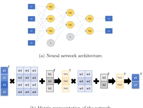
Figure 3.1(a) shows a fully connected neural network [27] with one single hidden layer. In this figure, the input and output of the network are represented by rectan-gular boxes. The neurons are represented by circles and the weights are depicted by the links between the neurons. Bias nodes are a constant input of one. The neurons will have a bias weight that is summed with the other links. These are indicated by shaded circles in Figure 3.1(a).
(a) Neural network architecture.
(b) Matrix representation of the network.
Fig. 3.1. Fully connected network with one input layer, one hidden layer and one output layer.
A fully connected layer can be viewed as a matrix multiplication between a 1xN input matrix and an NxM weights matrix. The result is a 1xM matrix. The bias 1xM matrix is then added to the previous result. This process is shown in Figure 3.1(b).
The main two operations associated with the network are forward propagation and backward propagation. These two operations are used during training to update the weights. Once the weights of the network are determined, the forward propagation is used on a new input to generate the estimated output.
3.1.1 Forward Propagation
In the forward propagation process, the output of each layer is generated by using Equation (3.1)
Where, X(1,N) is the input vector with N elements, W(N,M) is the weight matrix, and B(1,M) is the bias vector for the layer. The bias values in Equation (3.1) are added to the weighted term X(1xN)∗W(N xM) resulting in an output vector with M elements, Y(1,M).
Equation (3.1) is implemented in Algorithm 1.
Algorithm 1Forward Propagation in a Fully Connected Layer Input: X, W, B Matrix Output: Y Matrix 1: function ForwadPropagationFullyConnected(X, Y, W, B) 2: for n= 0 to len(Y) do 3: for m= 0 to len(X) do 4: sum←sum+W[n][m]∗X[m] 5: Y[n]←sum+B[n] 3.1.2 Backward Propagation
Backward Propagation [28] is used to train the network. It consists of three functions:
• The first function takes the output error it receives from the next layer and uses it to calculate the errors associated with the input it received from the previous layer (Equation 3.2a),
• The second function accumulates the errors for the weights of each neuron (Equation 3.2b), and
∆X(1(t)xN) = ∆Y(1(txM) )∗(W(t))T(M xN) (3.2a) ∆W((N xMt) ) = (X(t))T(N x1)∗∆Y(1(txM) ) (3.2b) ∆B(1(t)xN)= ∆Y(1(txN) ) (3.2c) Where, ∆X(1(t)xN) is the vector that holds the error due to the output ∆Y(1(txM) )
propagated back from the previous layer. ∆W((N xMt) ) represents the error matrix for the weights of the current layer. It will be used to adjust the current layer’s weights during training. ∆B(1(t)xM) is the error vector for the bias vector. It is used to adjust the bias vector during training. X(1(t)xM) is the input andW((N xMt) ) is the weight matrix of the current layer from the previous iteration of the algorithm. Equation (3.2) is implemented in Algorithm 2.
Algorithm 2Fully Connected Back Propagation
Input: dY, X, W Matrix
Output: dX, dW, dB Matrix
1: function FCBackProp(dY, dW, dB, X, W, dX) 2: SetToZero(dX) 3: for n= 0 to len(dY) do 4: for m= 0 to len(dX) do 5: dX[m]←dX[m] +W[n][m]∗dY[n] 6: dW[m][n]←X[m]∗dY[n] 7: dB[n]←dY[n] 3.2 Convolution Layer
The convolution layer [29] is very similar to the fully connected layer. However, instead of each neuron having a weight for each input, and only one output. Each neu-ron will have a volume of weights that step through the input in multiple dimensions with each step returning an output value.
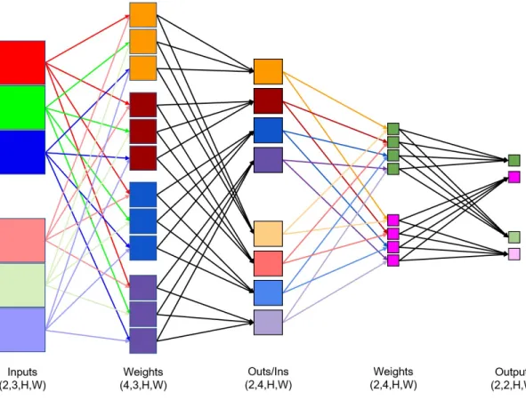
A typical architecture for a convolution layer receives a 4D input volume called a tensor with a format of NHWC or NCHW [30]. NHWC represents a tensor’s ordering by batch, height, width, and channel, respectively. For example, a NHWC tensor of bytes with the dimensions [20,320,240,4] is used to process a batch of 20 images with a height of 320 and width of 240. The 32 bit color information is represented as 4 byte color vector. Under NCHW, the dimensions would look like [20,4,320,240] with the pixels separated out into 4 feature maps, with a height of 320 and a width of 240. Performance can vary depending on the tensor format. For example, Intel rec-ommends NCHW for their newer processors [31], and Nvidia recrec-ommends NHWC in order to take advantage of the tensor core in their new architectures [32]. In this thesis NCHW is adopted, because it is easier to visualize.
The input, weights, and output should be in the same format. A convolution layer will contain a 4D tensor of weights. Under the adopted NCHW tensor format, N represents a batch of ”neurons” as opposed to a batch of inputs. The values stored in each CHW are the feature weights of N. These feature weights are also called kernels. The number of kernels is C, with a height of H and a width of W. For each neuron in W.N, there will be the same number of kernels (W.C) as there are feature maps from the input (X.C). The output tensor batch size is the same as the input’s batch size (i.e., N). The result of a neuron’s convolution of the input will be an output feature map with size HW. The number of neurons in the weights will determine the number of output feature maps. The size of the output channel dimension (Y.C) is determined by the number of neurons in the weights (W.N). The sizes of HW are determined by the properties of the convolution between the input and weights. An illustration of the 4D tensors in a convolutional neural network is shown in Figure 3.2.
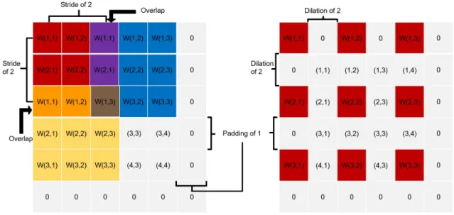
There are a few convolutional processing steps that are used in accessing the data being held by the input tensor. These are performed in the H and W dimensions and consist of padding, stride, and dilation. The properties of these data processing
Fig. 3.2. Schematic representation of 4D tensors. Each column is a tensor.
steps will affect the size of the output tensor. A visualization of the convolutional processing steps can be seen in Figure (3.3).
Padding (p) adds zeros around the H and W dimensions of the input tensor x. The size of the padding should be less than the size of the weights. If the padding is greater than or equal to the weights (w) then the output edges will be zeros.
Stride (s) corresponds to the step of the window over the input tensor in the H and W dimensions. Larger strides will reduce the size of the output.
Dilation (d) spreads the weights apart in the H and W dimensions giving them extended coverage without additional parameters.
As implied by the above three transformations, the shape of the output tensor is dependent on the parameters used to process the data. Equation (3.3) shows the size
of the output tensor based on the padding, stride, dilation. Not all parameter values can be used since some choices of p, w, s, d may lead to a non-integer size y for the output tensor. Therefore, best practice starts by fixing the sizeyof the output tensor and then deriving the sizex of the input tensor using Equation (3.4).
Fig. 3.3. A visualization of padding stride and dilation with an input of (4,4) and weights of (3,3).
y= x+ 2p−((w−1)∗d+ 1)
s + 1 (3.3)
x= (y−1)∗s−2p+ ((w−1)∗d+ 1) (3.4)
3.2.1 Forward Propagation
The values of the output tensor are calculated using Equation (3.5).
Yn,k,yh,yw(t) =Bk+ W.C−1 X c=0 W.H−1 X i=0 W.W−1 X j=0 Wk,c,i,j(t) ∗Xn,c,xh,xw(t) (3.5)
Where X represents the input tensor. W are the filter weights with k, c, i, j
representing the output channel size, input channel size, height position, and width position, respectively. Bk is a bias array. The size of the bias array is the same as
the size of the output channel k.
Padding is realized with Equation (3.6), where the values n, c, xh, and xw, are the batch size, channel size, height position, and width position, respectively. The height and width positions are calculated by using xh and xw as shown in Equation (3.7). In turn, xh and xw are calculated with respect to the output tensor position
yh, yw, slide (s), weight positions i, j, dilation (d), and padding offset (p).
Xn,c,xh,xw = Xn,c,xh,xw if 0≤xh < X.H and 0 ≤xw < X.W 0 otherwise (3.6) xh=yh∗s+i∗d−p, xw=yw∗s+j ∗d−p (3.7) The forward propagation function is executed into two steps. The first step is the sliding weight window over the input. This function returns the summation of the individual window as depicted in Algorithm 3. The second step stores the output of the previous layer as shown in Algorithm 4.
Algorithm 3Convolution Forward Window - Equation(3.5). Input: X, W Tensor
x input offset
n,k batch and neuron index d dilation size
Returns: sum summation of W*X window 1: function ConvForwardWin(X,W,x,n,k,d)
2: sum←0
3: for c= 0 to W.C do 4: for i= 0 to W.H do
5: xh←x.h+i∗d.h . add dilation height offset for X 6: if xh≥0 and xh < X.W then
7: for j = 0 to W.W do
8: xw←x.w+j∗d.w .add dilation width offset for X 9: if xw≥0 and xw < X.H then
10: sum←sum+W[k][c][i][j]∗X[n][c][xh][xw] return sum
Algorithm 4Convolution Forward Propagation Input: X, W, B Tensor
p, s, d Padding, stride and dilation sizes
Output: Y Tensor
1: function ConvForward( )
2: for n= 0 to Y.N do 3: for k = 0 to Y.C do
4: x.h← −p.h . set -padding height offset for X
5: for yh = 0 to Y.Hdo
6: x.w ← −p.w .set -padding width offset for X
7: x.h←x.h+yh∗s.h .add stride height offset for X
8: for yw= 0 to Y.W do
9: x.w←x.w+yw∗s.w . add stride width offset for X
10: sum←ConvF orwardW in(X, W, n, x, k, d)
3.2.2 Back Propagation
As in the case of a regular neural network, errors in a CNN are passed backward from the next layer. Each output error value is accumulated into two different tensors. The first is for the input tensor which is scaled according to the weights of each output as shown below. ∆Xn,c,xh,xw(t) = W.C−1 X c=0 W.H−1 X i=0 W.W−1 X j=0 Wk,c,i,j(t) ∗∆Yn,k,yh,yw(t) (3.8) Where, ∆X(t) is the tensor that holds the errors for X(t), W(t) is the weight tensor for the layer, and ∆Y(t) is the errors received forY(t). Equation (3.8) is implemented in Algorithm 5.
Algorithm 5Convolution Backward Data Window - Equation (3.8) Input: W Weight tensor
dy gradient
x input offset value n,k batch and neuron index d dilation size
Output: dX Input error tensor
1: function ConvInputGrad(dX, W, dy, x, n, k, d)
2: for c= 0 to W.C do 3: for i= 0 to W.H do 4: xh←x.h+i∗d.h 5: if xh≥0 and xh < X.W then 6: for j = 0 to W.W do 7: xw←x.w+j∗d.w 8: if xw≥0 and xw < X.H then 9: dX[n][c][xh][xw]←dX[n][c][xh][xw] +W[k][c][i][j]∗dy
The second tensor is an accumulation of errors used to update the weights. It is obtained by multiplying the input values by the corresponding output errors as shown below: ∆Wk,c,i,j(t) = W.C−1 X c=0 W.H−1 X i=0 W.W−1 X j=0 Xn,c,xh,xw(t) ∗∆Yn,k,yh,yw(t) (3.9) Where ∆W(t) is the tensor that holds the errors for the weights,X(t) is the input tensor for the layer, and ∆Y(t) represents the corresponding errors from the output. Equation (3.9) is implemented in Algorithm 6.
Algorithm 6Convolution Backward Weight Window - Equation (3.9) Input: X Input tensor
dy gradient
x input offset value n,k batch and neuron index d dilation size
Output: dW Weight update tensor
1: function ConvWeightGrad(dW, X, dy, x, n, k, d) 2: for c= 0 to W.C do 3: for i= 0 to W.H do 4: xh←x.h+i∗d.h 5: if xh≥0 and xh < X.W then 6: for j = 0 to W.W do 7: xw←x.w+j∗d.w 8: if xw≥0 and xw < X.H then 9: dW[k][c][i][j]←dW[k][c][i][j] +X[n][c][xh][xw]∗dy
The error for the bias neurons is the summation of the output errors for that neuron as shown below.
∆Bk(t)= Y.N−1 X n=0 Y.H−1 X yh=0 Y.W−1 X yw=0 ∆Yn,k,yh,yw(t) (3.10)
Where ∆B(t) is the tensor that holds the errors for the Bias, and ∆Y(t) is the output error.
Algorithm 7Convolution Back Propagation
Input: X, W, dY input, weight and output error tensors p, s, d padding, stride and dilation sizes Output: dX, dW, dB input, weight and bias update tensors 1: function ConvBackward(X, dX, W, dW, dB, dY, p, s, d)
2: ZeroAll(dX) 3: for n= 0 to Y.N do 4: for k = 0 to Y.C do 5: x.h← −p.h 6: for yh = 0 to Y.Hdo 7: x.w ← −p.w 8: x.h←x.h+yh∗s.h 9: for yw= 0 to Y.W do 10: x.w←x.w+yw∗s.w 11: dy←dY[n][k][yh][yw]
12: ConvInputGrad(dX, W, dy, n, x, k, d) . Algorithm 5
13: ConvW eightGrad(dW, X, dy, n, x, k, d) . Algorithm 6
3.3 Activation Layer
The activation layer introduces non-linearity to a neural network. This operation is performed element-wise. During forward propagation, the activation function is applied to the output of the previous layer. Some of the common activation functions include logistic (1+1e−x), rectified linear unit (Relu, if x ≤ 0 f(x) = 0, otherwise,
f(x) =x), and the leaky rectified linear unit (leaky, if x≤0 f(x) = 0.01, otherwise,
f(x) = x).
3.4 Weight Optimization
The weights in the network are updated at every training iteration. Several, approaches can be used to perform this update. Moreover, some of these approaches are guided by hyper-parameters that are either defined before training or adjusted during training. The choice of the hyper-parameters may dictate the ability of the network to converge. A summary of the main weight optimization approaches is provided next.
3.4.1 Gradient Descent
The simplest way to minimize the loss function at the output of the network is to update the weight in the direction of the gradient descent [33] as shown below.
W(t) =W(t−1)−∗∆W(t) (3.11) Where, W(t) is the updated weight value at iteration t, W(t−1) is the weight value at iterationt−1, and ∆W(t)is the weight error tensor. The hyper-parameter,, is called the learning rate and indicates the rate at which the updates are being performed.
3.4.2 Momentum Update
Compared to gradient descent, momentum update [28] takes into consideration the weight adjustment in the previous iterations as shown below:
M(t) =α∗M(t−1)−∗∆W(t) (3.12)
W(t)=W(t−1)+M(t) (3.13) Where, M(t) is the momentum at iteration t, M(t−1) is the momentum at the previous iteration,αis the momentum rate,is the learning rate,W(t)is the updated weight, W(t−1) is the weight at the previous iteration, and ∆W(t) is the weight error tensor. The hyper-parameters for this approach are and α.
3.4.3 Adagrad
Adagrad [34] stores the sum of the squares of the gradient for each individual parameter as shown in Equation (3.14). This value is then used to scale the gradient as shown in Equation (3.15). The hyper-parameter β in the Adagrad approach is used to prevent a divide by zero.
S(t)=S(t−1)+ (∆W(t))2 (3.14)
W(t) =W(t−1)+ −∗∆W (t)
√
S(t)+β (3.15)
Where, S(t) is the sum of the squares of the gradients at iteration t, S(t−1) is the squares of the gradients at iterationt−1, ∆W(t) is the weight error tensor,W(t)is the updated weight,W(t−1) is the weight value at the previous iteration, is the learning rate, and β is a meta parameter.
3.4.4 Adam
Adam [35] is a weight update approach that uses a large number of hyper-parameters and therefore, may require extensive tuning.
Ω(1t) =β1∗Ω (t−1) 1 + (1−β1)∗∆W(t) (3.16) Ω(1t)temp= Ω (t) 1 1−β1C+1 (3.17) Ω(2t)=β2∗Ω (t−1) 2 + (1−β2)∗(∆W(t))2 (3.18) Ω(2t)temp= Ω (t) 2 1−β2C+1 (3.19) W(t)=W(t−1)+ −(∗Ω (t) 1temp) q Ω(2t)temp+α (3.20) C(t) =C(t−1)+ 1 (3.21)
Where β1,β2,α, andare meta parameters, Ω1(t) and Ω(2t) are accumulated values that are updated during every iteration, C is a counter, ∆W(t) is the weight error tensor, W(t) is the weight tensor for the current iteration, and W(t−1) is the weight tensor from the previous iteration.
3.5 Implementation
The CNN was initially implemented in Go and executed on a regular CPU. The advantage of Go is that it has built-in concurrency and is supported by several APIs for image processing. Unfortunately, the performance of this implementation was not practical. In order to increase performance, the compute intensive section of the algorithm was migrated to a GPU implementation using CUDA.
The Go language has a pseudo-package ”CGO” [36] which was used to allow the front end of the application to call C functions including libraries that are compatible with GCC. This was necessary as an intermediary step. CUDA is based on CPP with few extensions. CUDA code is not directly compiled with GCC. CUDA code is compiled using NVCC. Therefore, CUDA kernels cannot be directly accessed using the CGO driver.
This limitation can be addressed in three ways. The first approach consists of creating a static or shared library of the kernels made for the GPU. This approach was not ideal since it entails making changes to the CUDA kernels.
The second approach consists of pre-compiling kernels into a .ptx file using the ptx option in NVCC. PTX code is similar to assembly language code and is compatible with different NVIDIA GPU architectures.
The third approach would use directly the NVRTC library. This approach creates a run time library. This third approach is similar to the second approach but with added flexibility. CUDA code can be compiled into a ptx format during runtime. In fact, the compiler can directly use the NVRTC library.
After evaluation, the second approach was used, because of a feature involving CUDA Contexts made using NVRTC inconsistent.
In order to access the functions that are in ptx form, the Driver API needs to be used. Specifically, a module needs to be made. Modules are dynamically loaded packages. A module can be created using NewModuleData() found in sub-package of GoCudnn called cuda. MakeKernel() will return a *Kernel that uses the method (*Kernel)Launch() to execute the kernel with the name passed in MakeKernel().
In order to allocate memory to the GPU. The Malloc() function of the cudart sub-package is an option. This function allocates memory to the GPU and this memory is managed by Go’s garbage collector. In addition, Memcpy() is used to copy memory to or from the GPU.
Code examples can be seen in Appendices A, B, and C. Appendix A exposes a few lower level deep learning functions using the CPU. Appendix C exposes the lower level bindings that are used to execute kernels on a GPU. Appendix B exposes code that is used to build deep learning models for execution on a GPU.
4. RESULTS
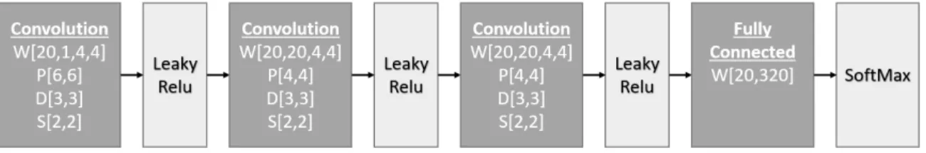
In order to test the results two different CNNs were built. One is using ConvNetGo, and the other is using GoCuNets. They are both based on the model seen in Figure (4.1). This model was chosen because it implements dilation, strides, and padding for each layer. The data being used is stored in a tensor with the dims of [N,1,28,28]. Each convolution has a filter with spacial dims [4,4], stride [2,2], and dilation [3,3]. The input Padding for the first convolution was set at [6,6] to make the output spacial dims [16,16]. The next two convolutions have a padding of [4,4]. The spatial dims of the output is half the size of the input. This convolution network is tested on an application that classifies hand-written digits. The final classification layer uses the input of the convolution layer and selects the digit that corresponds to the input image. This last layer consists of a fully connected layer with 10 neurons and 320 weights each. The digit image used to test the CNN implementation are extracted
Fig. 4.1. The layers of the CNN used to test the proposed framework.
from the MNIST [37] database. MNIST is a good benchmarking database for testing CNN models because it converges quickly. It consists of 60,000 training samples and 10,000 testing samples of hand written arabic numerals. Each sample has a size of 28 by 28. The target classification labels are stored as a byte of 0-9. Since, the model uses a softmax classifier, the output needs to be represented using one-hot encoding. An example is shown in Table (4.1).
Table 4.1.
Samples taken from the MNIST database with the corresponding one-hot encoding of their labels.
Input Target
[0,0,0,0,0,0,0,1,0,0]
[0,0,1,0,0,0,0,0,0,0]
[0,1,0,0,0,0,0,0,0,0]
[1,0,0,0,0,0,0,0,0,0]
Each network will run for 8 epochs. The average time it takes each epoch to complete is recorded along with the batch size. The ConvNetGo model is executed on a dual socket motherboard with two e5-2680v2 for a total of 20 cores and 40 threads. Each CPU has a 2.8 GHz clock with a boost clock of 3.6 GHz.
GoCuNets is executed on a GTX 1080ti GPU with a e5-2696v2 12 core / 24 thread CPU. The CPU has a 2.5 GHz base clock with a 3.3 GHz boost clock. The GPU has a base clock of 1.5 GHz and a boost of 1.6 GHz. Moreover, the GPU has 28 streaming multiprocessors with 128 CUDA cores each.
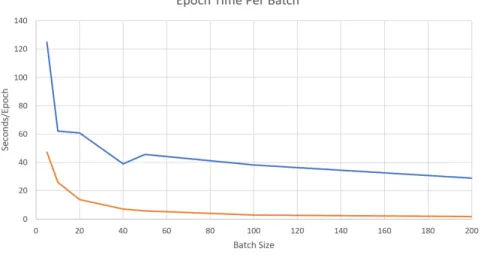
The execution times of the ConvNetGo and GoCuNets CNN classification models when applied to the MNIST database using different batches sizes are shown in Table 4.2. When the batch is set at 5, the model GoCuNes is twice as fast as ConvNetGo. When the batch increases to 5000, GoCuNets performs 57 times faster than Con-vNetGo. The execution times for the two CNNs are plotted against the batch size in Figure(4.2).
Table 4.2.
Execution time (in seconds) per epoch for each batch size for the Con-vNetGo (CPU implementation) and GoCuNets (GPU implementation).
Batch Size ConvNetGo GoCuNets CPU/GPU
5 124.97 47.23 2.11 10 61.97 25.94 1.91 20 60.67 13.77 3.52 40 39.02 7.09 4.40 50 45.68 5.58 6.55 100 38.05 2.81 10.83 200 28.95 1.65 14.03 400 27.13 0.98 22.15 500 27.46 0.81 27.12 1000 27.51 0.56 39.30 2000 27.92 0.43 51.95 5000 27.08 0.38 57.02
Table 4.3 shows the training time for the GoCuNets CNN with varying batch sizes. The training time is measured based on the same convergence criteria across all experiments. Each epoch consists of training and testing runs. The number of runs were determined by the size of the data-set divided by the batch size. The weights were trained during the training runs using the training data. The classification was then performed on the testing runs using the testing data. Training was complete when the average loss across the MNIST testing data-set is less than 0.01.
Fig. 4.2. Execution time per epoch for CoCuNets (GPU implementation) and ConvNetGo (CPU implementation) with increasing batch size.
4.1 Code Samples
Appendix A contains a few functions from ConvNetGo. These examples imple-ment some of the algorithms shown in this chapter. Appendix A.1 is an example of the data structure of a Tensor. Some methods and functions include Convolution Forward (Appendices A.2.2 and A.2.3), Fully Connected Forward (Appendix A.3.3), and Leaky Relu (Appendix A.3.2).
Appendix B contains a few functions from GoCuNets. It mostly covers the meth-ods that type Builder (Appendix B.2) uses. Builder is used to build deep learning models on a GPU. It contains methods such as ConvolutionLayer() (Appendix B.2.2) and Activation() (Appendix B.2.4) to create layers. These layers can be used to create structures that implement the Module Interface (Appendix B.3), like VanillaModule (Appendix B.3.1) and SimpleModuleNetwork (Appendix B.3.2).
Table 4.3.
Number of epochs, training time for each batch size when executing the GoCuNets (GPU) model. Convergence was decided when the average loss for the testing data was less than 0.01.
BatchSize N Epochs Learn Time (s)
5 8 377.84 10 7 181.58 20 6 82.62 40 9 63.81 50 9 50.22 100 11 30.91 200 15 24.75 400 22 21.56 500 25 20.25 1000 39 21.84 2000 62 26.66 5000 122 46.36
Appendix C contains a few samples taken from GoCudnn such as memory al-location on the GPU (Appendix C.7) and memory copy (Appendix C.8). The Ap-pendix also includes sample GPU io.Reader and io.Writer interfaces (ApAp-pendix C.9 and C.10). In addition, Appendix C shows the use of ConcatEX (Appendix C.6) to execute a concat kernel (Appendix C.3) using (*Kernel)Launch() (Appendix C.5).
5. CONCLUSION
The proposed GoCuNets shows that deep learning can be implemented using Go and GPUs. In fact, GoCuNets was able to achieve fast learning times. For instance, for the number digit classification application, the network converges in 25 epochs to an average loss less than .01. The total execution time for all epochs is 20.25 seconds with a batch size equal to 500. Assuming, ConvNetGo takes the same number of epochs to converge, a smaller batch size of 40 would require 5 minutes and 51 seconds. By using GPUs, GoCuNets makes developing deep learning models in Go a practical option.
5.1 Challenges
Creating and using custom kernels is not very intuitive. Using NVCC to generate a ptx file for custom kernels, and copying the contents of the ptx file into a constant string literal in a Go package makes creating GPU kernels challenging.
Launching a GPU kernel also requires several setup steps. These steps include allocating CPU and GPU memory, assigning values to the CPU memory, and then copying the values from CPU to GPU. Except for single value constants, this process has to be done for every value passed to a kernel. Moreover, when launching a kernel, the user must specify the number of blocks per grid and the number of threads per block. Finally, in order to evaluate a returned value on the CPU, the corresponding memory needs to be copied from the GPU back to the CPU.
5.2 Future Work
There are several directions for future work. Even though a large speed-up was achieved using a GPU, additional speed-up can be achieved by using multiple GPUs in parallel.
Moreover, the only GPUs currently supported under GoCuNets are Nvidia’s. Ei-ther integrating AMD GPUs into GoCuNets or creating a new framework that sup-ports both Nvidia and AMD GPUs would make deep learning using Go more widely available.
5.3 GoCuNets
GoCuNets is a GPU centric deep learning framework written in Go. It is available at www.github.com/dereklstinson/gocunets.
GoCudnn are bindings for Cuda. These bindings are used in GoCuNets. The package is available at www.github.com/dereklstinson/gocudnn.
ConvNetGo is a CPU centric deep learning framework written in Go. It uses Go’s built in concurrency to execute deep learning models. It is available at
REFERENCES
[1] “Go frequently asked questions (faq),” last accessed: 05/07/2020. [Online]. Available: https://golang.org/doc/faq
[2] “Go codetools,” last accessed: 05/07/2020. [Online]. Available: https: //github.com/golang/go/wiki/CodeTools
[3] M. Abadi, A. Agarwal, P. Barham, E. Brevdo, Z. Chen, C. Citro, G. S. Corrado, A. Davis, J. Dean, M. Devin, S. Ghemawat, I. Goodfellow, A. Harp, G. Irving, M. Isard, Y. Jia, R. Jozefowicz, L. Kaiser, M. Kudlur, J. Levenberg, D. Man´e, R. Monga, S. Moore, D. Murray, C. Olah, M. Schuster, J. Shlens, B. Steiner, I. Sutskever, K. Talwar, P. Tucker, V. Vanhoucke, V. Vasudevan, F. Vi´egas, O. Vinyals, P. Warden, M. Wattenberg, M. Wicke, Y. Yu, and X. Zheng, “TensorFlow: Large-scale machine learning on heterogeneous systems,” 2015, last accessed: 05/07/2020. [Online]. Available: https://www.tensorflow.org/ [4] A. Paszke, S. Gross, S. Chintala, G. Chanan, E. Yang, Z. DeVito,
Z. Lin, A. Desmaison, L. Antiga, and A. Lerer, “Automatic differentiation in pytorch,” 2017, last accessed: 05/07/2020. [Online]. Available: https: //openreview.net/pdf?id=BJJsrmfCZ
[5] F. Chollet et al., “Keras,” 2015, last accessed: 05/07/2020. [Online]. Available: https://keras.io
[6] T. Chen, M. Li, Y. Li, M. Lin, N. Wang, M. Wang, T. Xiao, B. Xu, C. Zhang, and Z. Zhang, “Mxnet: A flexible and efficient machine learning library for heterogeneous distributed systems,” 2015, last accessed: 05/07/2020. [Online]. Available: https://arxiv.org/abs/1512.01274
[7] S. Tokui, R. Okuta, T. Akiba, Y. Niitani, T. Ogawa, S. Saito, S. Suzuki, K. Uenishi, B. Vogel, and H. Yamazaki Vincent, “Chainer: A deep learning framework for accelerating the research cycle,” in Proceedings of the 25th ACM SIGKDD International Conference on Knowledge Discovery & Data Mining. ACM, 2019, pp. 2002–2011, last accessed: 05/07/2020. [Online]. Available: https://arxiv.org/abs/1908.00213
[8] “Gonum,” last accessed: 05/07/2020. [Online]. Available: https://www.gonum. org/
[9] “Gocv,” last accessed: 05/07/2020. [Online]. Available: https://gocv.io/
[10] D. Stinson, “Convnetgo,” last accessed: 05/07/2020. [Online]. Available: https://github.com/dereklstinson/convnetgo
[11] S. Chetlur, C. Woolley, P. Vandermersch, J. Cohen, J. Tran, B. Catanzaro, and E. Shelhamer, “cudnn: Efficient primitives for deep learning,” 2014.
[12] D. Stinson, “Gocudnn,” last accessed: 05/07/2020. [Online]. Available: https://github.com/dereklstinson/GoCudnn
[13] “Hip,” last accessed: 05/07/2020. [Online]. Available: https://github.com/ ROCm-Developer-Tools/HIP
[14] D. Stinson, “Hipgo,” last accessed: 05/07/2020. [Online]. Available: https://github.com/dereklstinson/hip
[15] J. Khan, P. Fultz, A. Tamazov, D. Lowell, C. Liu, M. Melesse, M. Nandhimandalam, K. Nasyrov, I. Perminov, T. Shah, V. Filippov, J. Zhang, J. Zhou, B. Natarajan, and M. Daga, “Miopen: An open source library for deep learning primitives,” 2019, last accessed: 05/07/2020. [Online]. Available: https://arxiv.org/abs/1910.00078
[16] D. Stinson, “Miopengo,” last accessed: 05/07/2020. [Online]. Available: https://github.com/dereklstinson/miopen
[17] D. L. Stinson, “Gocunets,” last accessed: 05/07/2020. [Online]. Available: https://github.com/dereklstinson/GoCuNets
[18] Barnex, “Cuda5,” last accessed: 05/07/2020. [Online]. Available: https: //github.com/barnex/cuda5
[19] “Gorgoniacu,” last accessed: 05/07/2020. [Online]. Available: https: //github.com/gorgonia/cu
[20] “Unixpckle/cuda,” last accessed: 05/07/2020. [Online]. Available: https: //github.com/unixpickle/cuda
[21] J. Nickolls, I. Buck, M. Garland, and K. Skadron, “Scalable parallel programming with cuda,” Queue, vol. 6, no. 2, p. 40–53, 2008. [Online]. Available: https://doi.org/10.1145/1365490.1365500
[22] “Go’s release history,” last accessed: 05/07/2020. [Online]. Available: https://golang.org/doc/devel/release.html
[23] Y. Jia, E. Shelhamer, J. Donahue, S. Karayev, J. Long, R. Girshick, S. Guadarrama, and T. Darrell, “Caffe: Convolutional architecture for fast feature embedding,” arXiv preprint arXiv:1408.5093, 2014, last accessed: 05/07/2020. [Online]. Available: https://arxiv.org/abs/1408.5093
[24] “Caffe 2,” last accessed: 05/07/2020. [Online]. Available: https://caffe2.ai/ blog/2017/04/18/caffe2-open-source-announcement.html
[25] A. Karpathy, “Convnetjs,” last accessed: 05/07/2020. [Online]. Available: https://github.com/karpathy/convnetjs
[26] “Gorgonia,” last accessed: 05/07/2020. [Online]. Available: https://gorgonia. org/
[27] “Fully connected layer,” last accessed: 05/07/2020. [Online]. Available: https://www.mathworks.com/help/deeplearning/ref/nnet.cnn.layer. fullyconnectedlayer.html
[28] G. O. Y. LeCun, L. Bottou and K. Muller, “Efficient backprop,” in Neural Net-works Tricks of the trade. Springer, 1998.
[29] Y. Lecun, L. Bottou, Y. Bengio, and P. Haffner, “Gradient-based learning applied to document recognition,” Proceedings of the IEEE, vol. 86, no. 11, pp. 2278– 2324, 1998.
[30] CUDNN DEVELOPERS GUIDE. Nvidia, 2020, last accessed: 05/07/2020. [Online]. Available: https://docs.nvidia.com/deeplearning/sdk/ cudnn-developer-guide/index.html
[31] E. O., TensorFlow* Optimizations on Modern IntelR Architecture. Intel, 2017, last accessed: 05/07/2020. [Online]. Available: https://software.intel. com/en-us/articles/tensorflow-optimizations-on-modern-intel-architecture [32] Deep Learning Performance Guide. Nvidia, 2019, last accessed:
05/07/2020. [Online]. Available: https://docs.nvidia.com/deeplearning/sdk/ dl-performance-guide/index.html
[33] Y. Bengio, “Practical recommendations for gradient-based training of deep architectures,” CoRR, vol. abs/1206.5533, 2012. [Online]. Available: http://arxiv.org/abs/1206.5533
[34] J. Duchi, E. Hazan, and Y. Singer, “Adaptive subgradient methods for online learning and stochastic optimization,” J. Mach. Learn. Res., vol. 12, pp. 2121–2159, Jul. 2011. [Online]. Available: http://dl.acm.org/citation.cfm?id= 1953048.2021068
[35] D. P. Kingma and J. Ba, “Adam: A method for stochastic optimization,” a conference paper at the 3rd International Conference for Learning Representations, San Diego, 2015, 2014, last accessed: 05/07/2020. [Online]. Available: https://arxiv.org/abs/1412.6980
[36] “Command cgo,” last accessed: 05/07/2020. [Online]. Available: https: //golang.org/cmd/cgo/
[37] Y. LeCun, C. Cortes, and C. Burges, “Mnist handwritten digit database,” ATT Labs [Online]. Available: http://yann. lecun. com/exdb/mnist, vol. 2, 2010.
A. CONVNETGO
A.1 Tensor 1 t y p e Tensor s t r u c t { 2 dims [ ]i n t 3 s t r i d e [ ]i n t 4 f 3 2 d a t a [ ]f l o a t 3 2 5 nhwc b o o l 6 } A.2 ConvolutionA.2.1 Convolution Struct
1 // C o n v o l u t i o n c o n t a i n s t h e p a r a m e t e r s 2 // t h a t a r e u s e d t o do a c o n v o l u t i o n 3 t y p e C o n v o l u t i o n s t r u c t { 4 padding , d i l a t i o n , s t r i d e [ ]i n t 5 s e t b o o l 6 nhwc b o o l 7 }
A.2.2 Convolution Forward Algorithm 1 f u n c ( c ∗C o n v o l u t i o n ) convnhwc4dwithwindow ( x , w, wb , y ∗Tensor ) { 2 v a r wg s y n c . WaitGroup 3 f o r yn := 0 ; yn < x . dims [ 0 ] ; yn++ { 4 wg . Add ( 1 ) //Add t o w a i t g r o u p 5 go f u n c( yn i n t) { // c o n c u r r e n t e x e c u t i o n 6 sh := −c . padding [ 0 ] 7 f o r yh := 0 ; yh < y . dims [ 1 ] ; yh++ { 8 sw := −c . padding [ 1 ] 9 f o r yw := 0 ; yw < y . dims [ 2 ] ; yw++ { 10 f o r yc := 0 ; yc < y . dims [ 3 ] ; yc++ { 11 dh , dw := c . d i l a t i o n [ 0 ] , c . d i l a t i o n [ 1 ] 12 a d d e r := c . fwdwinnhwc4d ( x , w, 13 sh , sw , dh , dw , yn , yc ) 14 a d d e r += wb . f 3 2 d a t a [ wn ] // add t h e b i a s 15 y . S e t ( adder , [ ]i n t{yn , yh , yw , yc}) 16 } 17 sw += c . s t r i d e [ 1 ] 18 } 19 sh += c . s t r i d e [ 0 ] 20 } 21 wg . Done ( )// g i v e done s i g n a l 22 }( yn )// end o f c o n c u r r e n t f u n c t i o n 23 } 24 wg . Wait ( )// Wait f o r t h r e a d s t o f i n i s h . 25 }
A.2.3 Convolution Forward Window 1 f u n c ( c ∗C o n v o l u t i o n ) fwdwinnhwc4d ( 2 x , w ∗Tensor , 3 sh , sw , dh , dw i n t , 4 xn , wn i n t) ( a d d e r f l o a t 3 2) { 5 6 f o r wh := 0 ; wh < w . dims [ 1 ] ; wh++ { 7 xh := sh + (wh ∗ dh ) 8 i f xh >= 0 && xh < x . dims [ 1 ] { 9 f o r ww := 0 ; ww < w . dims [ 2 ] ; ww++ { 10 xw := sw + (ww ∗ dw) 11 i f xw >= 0 && xw < x . dims [ 2 ] { 12 f o r wc := 0 ; wc < w . dims [ 3 ] ; wc++ { 13 a d d e r += x . f 3 2 d a t a [ ( x . s t r i d e [ 0 ]∗xn)+ 14 ( x . s t r i d e [ 1 ]∗xh)+ 15 ( x . s t r i d e [ 2 ]∗xw)+ 16 ( x . s t r i d e [ 3 ]∗wc ) ] ∗ 17 w . f 3 2 d a t a [ ( w . s t r i d e [ 0 ]∗wn)+ 18 (w . s t r i d e [ 1 ]∗wh)+ 19 (w . s t r i d e [ 2 ]∗ww)+ 20 (w . s t r i d e [ 3 ]∗wc ) ] 21 } 22 } 23 } 24 } 25 } 26 r e t u r n a d d e r 27 }
A.3 Leaky
A.3.1 Leaky Struct
1 // LeakyRelu i s a s t r u c t t h a t h o l d s t h e neg and p o s c o e f
2 t y p e LeakyRelu s t r u c t {
3 n e g c o e f , p o s c o e f f l o a t 3 2
4 }
A.3.2 Leaky Forward
1 f u n c ( l ∗LeakyRelu ) Forward ( x , y ∗Tensor ) ( e r r e r r o r) {
2 n b a t c h e s := x . dims [ 0 ] 3 n b a t c h e l e m e n t s := x . s t r i d e [ 0 ] 4 v a r wg s y n c . WaitGroup 5 f o r i := 0 ; i < n b a t c h e s ; i++ { 6 wg . Add ( 1 ) 7 b a t c h o f f s e t := i ∗ n b a t c h e l e m e n t s 8 go f u n c( b a t c h o f f s e t , n b a t c h e l e m e n t s i n t) { 9 f o r j := 0 ; j < n b a t c h e l e m e n t s ; j++ { 10 i f x . f 3 2 d a t a [ b a t c h o f f s e t+j ] < 0 { 11 y . f 3 2 d a t a [ b a t c h o f f s e t+j ] = 12 x . f 3 2 d a t a [ b a t c h o f f s e t+j ] ∗ l . n e g c o e f 13 } e l s e { 14 y . f 3 2 d a t a [ b a t c h o f f s e t+j ] = 15 x . f 3 2 d a t a [ b a t c h o f f s e t+j ] ∗ l . p o s c o e f 16 } 17 } 18 wg . Done ( ) 19 }( b a t c h o f f s e t , n b a t c h e l e m e n t s ) 20 } 21 wg . Wait ( ) 22 r e t u r n n i l 23 }
A.3.3 Fully Connected 1 f u n c F u l l y C o n n e c t e d F o r w a r d ( x , w, b , y ∗Tensor ) e r r o r { 2 n v o l := f i n d v o l u m e (w . dims [ 1 : ] ) 3 x b a t c h s t r i d e := x . s t r i d e [ 0 ] 4 y b a t c h s t r i d e := y . s t r i d e [ 0 ] 5 n e u r o n s := w . dims [ 0 ] 6 v a r wg s y n c . WaitGroup 7 f o r i := 0 ; i < x . dims [ 0 ] ; i++ { 8 wg . Add ( 1 ) 9 go f u n c( i i n t) { 10 y o f f s e t := y b a t c h s t r i d e ∗ i 11 x b o f f s e t := x b a t c h s t r i d e ∗ i 12 f o r j := 0 ; j < n e u r o n s ; j++ { 13 n e u r o n o f f s e t := w . s t r i d e [ 0 ] ∗ j 14 v a r a d d e r f l o a t 3 2 15 f o r k := 0 ; k < x b a t c h s t r i d e ; k++ { 16 a d d e r += w . f 3 2 d a t a [ n e u r o n o f f s e t+k ] 17 ∗ x . f 3 2 d a t a [ x b o f f s e t+k ] 18 } 19 y . f 3 2 d a t a [ y o f f s e t+j ] = a d d e r + b . f 3 2 d a t a [ j ] 20 } 21 wg . Done ( ) 22 }( i ) 23 } 24 wg . Wait ( ) 25 r e t u r n n i l 26 }
B. GOCUNETS
B.1 Tensor 1 t y p e Tensor s t r u c t { 2 ∗l a y e r s . Tensor 3 i d i n t 6 4 4 to , from Module 5 } 1 // Layer i s a l a y e r i n s i d e a n e t w o r k i t h o l d s i n p u t s and o u t p u t s 2 t y p e Layer s t r u c t { 3 i d i n t 6 4 4 name s t r i n g 5 h ∗Handle 6 op O p e r a t i o n 7 workspacefwd ∗n v i d i a . M a l l o c e d 8 workspacebwd ∗n v i d i a . M a l l o c e d 9 workspacebwf ∗n v i d i a . M a l l o c e d 10 x , dx , y , dy ∗Tensor 11 }B.2 Builder
B.2.1 Builder Data Structure
1 // B u i l d e r w i l l c r e a t e l a y e r s w i t h t h e f l a g s s e t w i t h i n t h e s t r u c t 2 t y p e B u i l d e r s t r u c t { 3 h ∗Handle 4 gpurng ∗curand . G e n e r a t o r 5 Frmt TensorFormat 6 Dtype DataType 7 Cmode ConvolutionMode 8 Mtype MathType 9 Pmode PoolingMode 10 AMode A c t i v a t i o n M o d e 11 BNMode BatchNormMode 12 Nan NanProp 13 c u r n g t y p e curand . RngType 14 }
B.2.2 Builder Method Convolution Layer
1 // C o n v o l u t i o n L a y e r c r e a t e s a c o n v o l u t i o n l a y e r
2 f u n c ( l ∗B u i l d e r ) C o n v o l u t i o n L a y e r (
3 i d i n t 6 4 , g r o u p c o u n t i n t 3 2,
4 w, dw , b , db ∗Tensor ,
5 pad , s t r i d e , d i l a t i o n [ ]i n t 3 2) ( conv ∗Layer , e r r e r r o r) {
6 c l a y e r , e r r := cnn . S e t u p B a s i c ( 7 l . h . Handler , 8 l . Frmt . TensorFormat , 9 l . Dtype . DataType , 10 l . Mtype . MathType , 11 groupcount ,
12 w . Tensor , dw . Tensor , b . Tensor , db . Tensor , 13 l . Cmode . ConvolutionMode , 14 pad , 15 s t r i d e , 16 d i l a t i o n ) 17 i f e r r != n i l { 18 r e t u r n n i l , e r r 19 } 20 conv , e r r = c r e a t e l a y e r ( i d , l . h , c l a y e r ) 21 i f e r r != n i l { 22 r e t u r n n i l , e r r 23 } 24 r e t u r n conv , n i l 25 }
B.2.3 Builder Method Convolution Weights 1 // C r e a t e C o n v o l u t i o n W e i g h t s c r e a t e s t h e w e i g h t s and 2 // d e l t a w e i g h t s o f a c o n v o l u t i o n l a y e r 3 f u n c ( l ∗B u i l d e r ) C r e a t e C o n v o l u t i o n W e i g h t s ( dims [ ]i n t 3 2) ( 4 w, dw , b , db ∗Tensor , e r r e r r o r) { 5 w, e r r = l . C r e a t e T e n s o r ( dims ) 6 i f e r r != n i l { 7 r e t u r n n i l , n i l , n i l , n i l , e r r 8 } 9 dw , e r r = l . C r e a t e T e n s o r ( dims ) 10 i f e r r != n i l { 11 r e t u r n n i l , n i l , n i l , n i l , e r r 12 } 13 b , e r r = l . C r e a t e B i a s T e n s o r ( dims ) 14 i f e r r != n i l { 15 r e t u r n n i l , n i l , n i l , n i l , e r r 16 } 17 db , e r r = l . C r e a t e B i a s T e n s o r ( dims ) 18 i f e r r != n i l { 19 r e t u r n n i l , n i l , n i l , n i l , e r r 20 } 21 r e t u r n w, dw , b , db , n i l 22 }
B.2.4 Builder Method Activation Layer 1 // A c t i v a t i o n c r e a t e s an a c t i v a t i o n l a y e r 2 f u n c ( l ∗B u i l d e r ) A c t i v a t i o n ( i d i n t 6 4) ( a ∗Layer , e r r e r r o r) { 3 v a r a c t ∗a c t i v a t i o n . Layer 4 a f l g := l . AMode 5 s w i t c h l . AMode { 6 c a s e a f l g . Leaky ( ) :
7 a c t , e r r = a c t i v a t i o n . Leaky ( l . h . Handler , l . Dtype . DataType )
8 c a s e a f l g . C l i p p e d R e l u ( ) :
9 a c t , e r r = a c t i v a t i o n . C l i p p e d R e l u ( l . h . Handler , 10 l . Dtype . DataType )
11 c a s e a f l g . Relu ( ) :
12 a c t , e r r = a c t i v a t i o n . Relu ( l . h . Handler , l . Dtype . DataType )
13 c a s e a f l g . Elu ( ) :
14 a c t , e r r = a c t i v a t i o n . Elu ( l . h . Handler , l . Dtype . DataType )
15 c a s e a f l g . Sigmoid ( ) :
16 a c t , e r r = a c t i v a t i o n . Sigmoid ( l . h . Handler , l . Dtype . DataType )
17 c a s e a f l g . Tanh ( ) :
18 a c t , e r r = a c t i v a t i o n . Tanh ( l . h . Handler , l . Dtype . DataType )
19 d e f a u l t: 20 r e t u r n n i l , e r r o r s . New(” A p p e n d A c t i v a t i o n : ”+ 21 ” Not s u p p o r t e d A c t i v a t i o n Layer ”) 22 } 23 i f e r r != n i l { 24 r e t u r n n i l , e r r 25 } 26 a , e r r = c r e a t e l a y e r ( i d , l . h , a c t ) 27 28 r e t u r n a , e r r 29 }
B.3 Module Interface
1 // Module i s a wrapper around
2 // a n e u r a l n e t w o r k o r s e t o f o p e r a t i o n s 3 t y p e Module i n t e r f a c e { 4 ID ( )i n t 6 4 5 Forward ( ) e r r o r 6 Backward ( ) e r r o r 7 FindOutputDims ( ) ( [ ]i n t 3 2, e r r o r) 8 I n f e r e n c e ( ) e r r o r 9 I n i t H i d d e n L a y e r s ( ) ( e r r e r r o r) 10 I n i t W o r k s p a c e ( ) ( e r r e r r o r) 11 GetTensorX ( ) ( x ∗Tensor ) 12 GetTensorDX ( ) ( dx ∗Tensor ) 13 GetTensorY ( ) ( y ∗Tensor ) 14 GetTensorDY ( ) ( dy ∗Tensor ) 15 SetTensorX ( x ∗Tensor ) 16 SetTensorDX ( dx ∗Tensor ) 17 SetTensorY ( y ∗Tensor ) 18 SetTensorDY ( dy ∗Tensor ) 19 }
B.3.1 VanillaModule 1 // V a n i l l a M o d u l e h a s a c o n v o l u t i o n and an a c t i v a t i o n 2 t y p e V a n i l l a M o d u l e s t r u c t { 3 i d i n t 6 4 4 b ∗B u i l d e r 5 conv ∗Layer 6 a c t ∗Layer 7 } 1 // Forward s a t i s f i e s module i n t e r f a c e 2 f u n c (m ∗V a n i l l a M o d u l e ) Forward ( ) e r r o r { 3 e r r := m. conv . Forward ( ) 4 i f e r r != n i l { 5 r e t u r n e r r 6 } 7 r e t u r n m. a c t . Forward ( ) 8 }
B.3.2 ModuleNetwork 1 // SimpleModuleNetwork i s a s i m p l e module n e t w o r k 2 t y p e SimpleModuleNetwork s t r u c t { 3 i d i n t 6 4 4 Modules [ ] Module 5 Output ∗OutputModule 6 C l a s s i f i e r ∗C l a s s i f i e r M o d u l e 7 b ∗B u i l d e r 8 } 1 // Forward p e r f o r m s t h e f o r w a r d o p e r a t i o n 2 // o f t h e s i m p l e module n e t w o r k 3 // Forward s a t a s i f i e s t h e Module I n t e r f a c e . 4 f u n c (m ∗SimpleModuleNetwork ) Forward ( ) ( e r r e r r o r) { 5 f o r , mod := r a n g e m. Modules { 6 e r r = mod . Forward ( ) 7 i f e r r != n i l { 8 r e t u r n e r r 9 } 10 } 11 i f m. Output != n i l { 12 e r r = m. Output . Forward ( ) 13 i f e r r != n i l { 14 r e t u r n e r r 15 } 16 } 17 i f m. C l a s s i f i e r != n i l { 18 r e t u r n m. C l a s s i f i e r . P e r f o r m E r r o r ( ) 19 } 20 r e t u r n n i l 21 }
C. GOCUDNN
C.1 Linking Cuda to Go 1 p a c k a g e cuda 2 /∗ 3 #c g o LDFLAGS:−L/ u s r / l o c a l / cuda / l i b 6 4 −l c u d a 4 #c g o CFLAGS: −I / u s r / l o c a l / cuda / i n c l u d e / 5 ∗/ 6 i m p o r t ”C” C.2 NewModuleData1 // NewModuleData t a k e s a i o . Reader and c r e a t e s a Module w i t h i t .
2 f u n c NewModuleData ( r i o . Reader ) (∗Module , e r r o r) {
3 p t x b y t e s , e r r := i o u t i l . ReadAll ( r ) 4 i f e r r != n i l { 5 r e t u r n n i l , e r r 6 } 7 v a r mod C . CUmodule 8 c p t x := C . C S t r i n g (s t r i n g( p t x b y t e s ) ) 9 d e f e r C . f r e e ( ( u n s a f e . P o i n t e r ) ( c p t x ) ) 10 e r r = s t a t u s (C . cuModuleLoadData(&mod , 11 ( u n s a f e . P o i n t e r ) ( c p t x ) ) ) .e r r o r(”NewModuleData”) 12 r e t u r n &Module{ 13 m: mod , 14 l o a d e d : t r u e , 15 }, e r r 16 }
C.3 Cuda Concat Kernel 1 e x t e r n ”C” 2 g l o b a l v o i d ConcatNCHWEX(c o n s t i n t XThreads , 3 c o n s t i n t Batches , 4 c o n s t i n t DestBatchVol , 5 c o n s t i n t D e s t C h a n n e l O f f s e t , 6 f l o a t ∗s r c , 7 c o n s t f l o a t alpha , 8 c o n s t i n t SrcBatchVol , 9 f l o a t ∗d e s t , 10 c o n s t f l o a t beta , 11 b o o l f o r w a r d ){ 12 f o r (i n t i =0; i<B a t c h e s ; i ++){
13 GRID AXIS LOOP ( idX , XThreads , x ){
14 i n t d e s t s t r i d e = ( i∗DestBatchVol )+( D e s t C h a n n e l O f f s e t+idX ) ; 15 i n t s r c s t r i d e = ( i∗S r c B a t c h V o l )+( idX ) ; 16 i f ( f o r w a r d ){ 17 d e s t [ d e s t s t r i d e ]= s r c [ s r c s t r i d e ]∗a l p h a + d e s t [ d e s t s t r i d e ]∗b e t a ; 18 }e l s e{ 19 s r c [ s r c s t r i d e ]= d e s t [ d e s t s t r i d e ]∗a l p h a + s r c [ s r c s t r i d e ]∗b e t a ; 20 }}}}
C.4 MakeKernel
1 // MakeKernel makes a k e r n e l .
2 // kname i s t h e k e r n e l s name t h a t was w r i t t e n i n cuda .
3 f u n c MakeKernel ( kname s t r i n g , m ∗Module ) (
4 k ∗K er ne l , e r r e r r o r) {
5 v a r k e r n C . CUfunction
6 i f m. l o a d e d == f a l s e {
7 r e t u r n n i l , e r r o r s . New(” MakeKernel : Module Not Loaded ”)
8 }
9 name := C . C S t r i n g ( kname )
10 d e f e r C . f r e e ( ( u n s a f e . P o i n t e r ) ( name ) )
11 e r r = s t a t u s (
12 C . cuModuleGetFunction (& kern , m.m, name ) ) .e r r o r(” MakeKernel ”) 13 i f e r r != n i l { 14 r e t u r n n i l , e r r 15 } 16 k = &K e r n e l{ 17 name : kname , 18 m: m, 19 f : kern , 20 } 21 // Give k t o Go ’ s Garbage C o l l e c t o r 22 r u n t i m e . S e t F i n a l i z e r ( k , d e s t r o y c u d a k e r n e l ) 23 r e t u r n k , n i l 24 }
C.5 (k *Kernel) Launch() 1 // Launch w i l l l a u n c h a k e r n a l t h a t ’ s b e e n a s s i g n e d t o i t . 2 f u n c ( k ∗K e r n e l ) Launch ( gx , gy , gz , bx , by , bz , 3 s h a r e d u i n t 3 2 , s t r e a m gocu . Streamer , 4 a r g s . . . i n t e r f a c e{ }) e r r o r { 5 v a r s h o l d u n s a f e . P o i n t e r 6 i f s t r e a m != n i l { 7 s h o l d = s t r e a m . Ptr ( ) 8 } 9 c a r g s := m a k e l a u n c h a r g s (l e n( a r g s ) ) 10 e r r := k . i f a c e t o u n s a f e c o m p l e t e ( a r g s , c a r g s ) 11 i f e r r != n i l { 12 r e t u r n e r r 13 } 14 r e t u r n s t a t u s (C . cuLaunchKernel ( k . f , 15 C .u i n t( gx ) , C .u i n t( gy ) , C .u i n t( gz ) , 16 C .u i n t( bx ) , C .u i n t( by ) , C .u i n t( bz ) , 17 C .u i n t( s h a r e d ) , 18 (C . CUstream ) ( s h o l d ) , 19 &c a r g s . a r g s [ 0 ] , C . v o i d d p t r n u l l , 20 ) ) .e r r o r(” ( k ∗K e r n e l ) Launch ( ) ”) 21 22 }
C.6 Concat Kernel Launch
1 f u n c ( c ∗ConcatEx ) op ( h ∗Handle ,
2 s r c s [ ]∗gocudnn . TensorD , srcsmem [ ] c u t i l .Mem, 3 a l p h a f l o a t 6 4 ,
4 d e s t ∗gocudnn . TensorD , destmem c u t i l .Mem, 5 b e t a f l o a t 6 4 , f o r w a r d b o o l) e r r o r {
6 dfrmt , ddtype , ddims , , := d e s t . Get ( ) 7 b a t c h e s := ddims [ 0 ] 8 d e s t b a t c h v o l := f i n d v o l ( ddims [ 1 : ] ) 9 v a r s r c c h a n o f f s e t i n t 3 2 10 11 f o r i :=r a n g e s r c s{ 12 s r c d i m s := s r c s [ i ] . Dims ( ) 13 s r c b a t c h v o l := f i n d v o l ( s r c d i m s [ 1 : ] ) 14 a := f l o a t 3 2( a l p h a ) 15 b := f l o a t 3 2( b e t a ) 16 c o n f i g := h . LaunchConfig ( s r c b a t c h v o l ) 17 e r r = c . f p 3 2 . nchw . Launch ( 18 c o n f i g . BlockCount , 1 , 1 , // g r i d p a r a m e t e r s 19 c o n f i g . ThreadPerBlock , 1 , 1 , // b l o c k p a r a m e t e r s 20 0 , c . s t r e a m s [ i ] , // s h a r e d memory , s t r e a m 21 // r e s t a r e a r g u m e n t s 22 c o n f i g . Elements , b a t c h e s , 23 d e s t b a t c h v o l , s r c c h a n o f f s e t , 24 srcsmem [ i ] , 25 a , s r c b a t c h v o l , 26 destmem , b , f o r w a r d ) 27 i f e r r != n i l { 28 r e t u r n e r r 29 } 30 s r c c h a n o f f s e t += s r c b a t c h v o l 31 } 32 }
C.7 MallocManagedGlobalEx
1 // MallocManagedGlobalEx a l l o c a t e s memory t o 2 // d e v i c e a s s o c i a t e d w i t h w .
3 // I f w i s n i l t h e n i t w i l l
4 // b e h a v e l i k e M a l l o c M a n a g e d G l o b a l
5 f u n c MallocManagedGlobalEx (w ∗gocu . Worker ,
6 mem c u t i l .Mem, s i z e u i n t) e r r o r { 7 v a r e r r e r r o r 8 i f w != n i l { 9 e r r = w . Work (f u n c( ) e r r o r { 10 e r r = s t a t u s (C . cudaMallocManaged ( 11 mem. DPtr ( ) , C . s i z e t ( s i z e ) , 12 C . cudaMemAttachGlobal ) ) .e r r o r(” MallocManagedGlobalEx ”) 13 i f e r r != n i l { 14 r e t u r n e r r 15 } 16 r e t u r n Memset (mem, 0 , ( s i z e ) ) 17 }) 18 } e l s e { 19 e r r = s t a t u s (C . cudaMallocManaged (mem. DPtr ( ) , C . s i z e t ( s i z e ) , 20 C . cudaMemAttachGlobal ) ) .e r r o r(” MallocManagedGlobalEx ”) 21 i f e r r != n i l { 22 r e t u r n e r r 23 } 24 e r r = Memset (mem, 0 , ( s i z e ) ) 25 } 26 i f e r r != n i l { 27 r e t u r n e r r 28 }
29 // Put Go Garbage C o l l e c t o r i n c h a r g e o f CUDA memory . 30 r u n t i m e . S e t F i n a l i z e r (mem, d e v i c e f r e e m e m )
31 r e t u r n n i l
C.8 Copy Memory
1 //Memcpy c o p i e s some memory from s r c t o d e s t .
2 // I f d e f a u l t i s s e l e c t e d and i f t h e s y s t e m s u p p o r t s 3 // u n i f i e d v i r t u a l a d d r e s s i n g t h e n t h e t r a n s f e r i s i n f e r r e d . 4 f u n c Memcpy( d e s t , s r c c u t i l . P o i n t e r , s i z e t u i n t , 5 k i n d MemcpyKind ) e r r o r { 6 r e t u r n s t a t u s (C . cudaMemcpy ( d e s t . Ptr ( ) , s r c . Ptr ( ) , 7 C . s i z e t ( s i z e t ) , k i n d . c ( ) ) ) .e r r o r(”Memcpy”) 8 }
C.9 Interface io.Reader 1 // Read s a t i s f i e s t h e i o . Reader i n t e r f a c e 2 f u n c ( r ∗ReadWriter ) Read ( b [ ]b y t e) ( n i n t , e r r e r r o r) { 3 i f r . i >= r . s i z e { 4 r . R e s e t ( ) 5 r e t u r n 0 , i o .EOF 6 } 7 i f l e n( b ) == 0 { 8 r e t u r n 0 , n i l 9 } 10 v a r s i z e = r . s i z e − r . i 11 i f u i n t(l e n( b ) ) < s i z e { 12 s i z e = u i n t(l e n( b ) ) 13 }
14 bwrap , := c u t i l . WrapGoMem( b )// don ’ t need t o c h e c k e r r o r , 15 // b e c a u s e [ ] b y t e i s s u p p o r t e d by f u n c t i o n . 16 i f r . s != n i l { 17 e r r = c u d a r t . MemcpyAsync ( bwrap , c u t i l . O f f s e t ( r , r . i ) , 18 s i z e , r . c p f l g , r . s ) 19 } e l s e { 20 e r r = c u d a r t . Memcpy( bwrap , c u t i l . O f f s e t ( r , r . i ) , 21 s i z e , r . c p f l g ) 22 } 23 i f e r r != n i l { 24 r e t u r n 0 , n i l 25 } 26 r . i += s i z e 27 n = i n t( s i z e ) 28 r e t u r n n , n i l 29 }
C.10 Interface io.Writer
1 // Write s a t i s f i e s t h e i o . W r i t e r i n t e r f a c e
2 f u n c ( r ∗ReadWriter ) Write ( b [ ]b y t e) ( n i n t , e r r e r r o r) {
3 i f r . i >= r . s i z e {
4 r . R e s e t ( )
5 r e t u r n 0 , e r r o r s . New(” ( r ∗ReadWriter ) Write ( ) ” +
6 ” Write L o c a t i o n Out o f Memory”)
7 } 8 i f l e n( b ) == 0 { 9 r e t u r n 0 , n i l 10 } 11 v a r s i z e = r . s i z e − r . i 12 i f u i n t(l e n( b ) ) < s i z e { 13 s i z e = u i n t(l e n( b ) ) 14 }
15 bwrap , := c u t i l . WrapGoMem( b ) )// don ’ t need t o c h e c k e r r o r , 16 // b e c a u s e [ ] b y t e i s s u p p o r t e d by f u n c t i o n . 17 i f r . s != n i l { 18 e r r = c u d a r t . MemcpyAsync ( c u t i l . O f f s e t ( r , r . i ) , bwrap , 19 s i z e , r . c p y f l g , r . s ) 20 } e l s e { 21 e r r = c u d a r t . Memcpy( c u t i l . O f f s e t ( r , r . i ) , bwrap , 22 s i z e , r . c p t f l g ) 23 } 24 r . i += s i z e 25 n = i n t( s i z e ) 26 r e t u r n n , e r r 27 }