Full Bayesian Methods to Handle Missing Data in Health Economic Evaluation

(1)

Full Bayesian Methods to Handle

Missing Data in Health Economic

Evaluation

Andrea Gabrio

University College London (UCL)

Department of Statistical Science

A thesis presented for the degree of

Doctor of Philosophy in Statistics

(2)

Declaration of Authorship

I, Andrea Gabrio, confirm that the work presented in this thesis is my own. Where information has been derived from other sources, I confirm that this has been indicated in the thesis.

Signed: Date:

(3)

Abstract

Trial-based economic evaluations are performed on individual-level data, which almost invariably contain missing values. Missingness represents a threat for the analysis because any statistical method makes assumptions about the unobserved values that cannot be verified from the data at hand; when these assumptions are not realistic, they could lead to biased inferences and mislead the cost-effectiveness assessment.

We start by investigating the current missing data handling in economic evaluations and pro-vide recommendations about how information about missingness and related methods should be reported in the analysis. We illustrate the pitfalls and issues that affect the methods used in rou-tine analyses, which typically do not account for the intrinsic complexities of the data and rarely include sensitivity analysis to the missingness assumptions. We propose to overcome these prob-lems using a full Bayesian approach. We use two case studies to demonstrate the benefits of our approach, which allows for a flexible specification of the model to jointly handle the complexities of the data and the uncertainty around the missing values.

Finally, we present a longitudinal bivariate model to handle nonignorable missingness. The model extends the standard approach by accounting for all observed data, for which a flexible parametric model is specified. Missing data are handled through a combination of identifying restrictions and sensitivity parameters. First, a benchmark scenario is specified and then plau-sible nonignorable departures are assessed using alternative prior distributions on the sensitivity parameters. The model is applied to and motivated by one of the two case studies considered.

(4)

Impact Statement

My PhD research has focussed on the handling of missing data in health economic evaluation, mainly from a Bayesian statistical perspective. Through two real case examples, I have identi-fied the limitations of the standard approach used by practitioners and proposed an alternative statistical framework to perform economic evaluations that can improve the current practice. This has resulted in one first author publication and three original manuscripts that have already been submitted for publication to different academic journals.

My research has important implications within the health economics community due to the fact that considerable proportions of missing data often occur in trial-based analyses, but their impact on the results is rarely assessed. The results from this thesis show that failure to conduct sensi-tivity analysis to plausible missingness assumptions can have substantial implications in terms of decision-making and could lead to different cost-effectiveness assessments. This is a problem of great interest to many clinicians, health economists and, crucially, decision-makers (e.g. NICE in the UK), who typically use the results from these analyses to inform resource allocation decisions and the funding of new healthcare technologies. A statistical software package is under develop-ment to facilitate the impledevelop-mentation of the methods presented in this thesis in routine analyses among practitioners and make them available to a wider audience.

During my PhD I have been invited to present my work at the Centre for Statistical Method-ology Early Career Researcher Showcase (London School of Hygiene and Tropical Medicine, London, 2018). I have given oral presentations at the PRIMENT Statistics, Health Economics and Methodology Seminar (UCL, London, 2018) as well as poster presentations at the Third European Health Economics Association (EuHEA) PhD student-supervisor and early career re-searcher conference (Universitat Internacional de Catalunya, Barcelona, 2016) and at the Health Economics Symposium (UCL, London, 2018). I have also been awarded the Costas Goutis Prize (2017) and a research grant from the Foundation BLANCEFLOR Boncompagni - Ludovisi née Bildt (2015-2018).

(5)

List of Tables

1.1 Example of a typical trial-based dataset used in economic evaluations. . . 6 2.1 List of the information content for the three components to achieve a full reporting

of the missing data analysis. . . 33 2.2 Numerical scores associated with the level of the information content provided in

each component. . . 33 3.1 Number and proportion of observed utilities and costs at each time point in the

MenSS trial, presented by group. . . 47 3.2 Description of the available covariates in the MenSS trial . . . 49 3.3 Missingness patterns for the outcomeyij = (uij, cij)in the PBS study. . . 50 3.4 Number and proportion of observed utilities and costs at each time point in the PBS

trial, presented by group. . . 50 3.5 Description of the available covariates in the PBS trial. . . 52 4.1 List of the different models compared in the analysis of the MenSS and PBS data. 60 4.2 Posterior means and 95% credible intervals of the mean QALYs and cost

parame-ters in the MenSS trial. . . 61 4.3 Posterior means and 95% credible intervals of the mean QALYs and cost

parame-ters in the PBS trial. . . 63 5.1 Alternative MNAR scenarios considered in the MenSS study for the Hurdle Model. 76 5.2 DIC and pD for each variable in the Bivariate Normal, Beta-Gamma and Hurdle

Model fitted to the MenSS data. . . 77 5.3 DIC andpDfor each variable in the Bivariate Normal, Beta-LogNormal and Hurdle

Model fitted to the PBS data. . . 85 6.1 Utility and cost data for thei-th subject at each timejderived from a subset of the

first 10 subjects in the PBS study. . . 94 6.2 DIC andpDvalues associated with each variable in the model. . . 102 6.3 List of the scenarios compared in the analysis of the PBS study. . . 103 C.1 Comparison of three weighting schemes, based on the information provided on

missingness in each component of the analysis: Description (D), Method (M) and Limitations (L) . . . 141

(10)

C.2 Scoring system associated with each group category in three weight allocation ver-sions of the Quality Evaluation Scheme. . . 141 C.3 Missing cost articles distribution (total number of articles = 81) across the

cate-gories of the Quality Evaluation Scheme for the three weight allocation versions compared. . . 142 C.4 Missing effect articles distribution (total number of articles = 81) across the

cat-egories of the Quality Evaluation Scheme for the three weight allocation versions compared. . . 142 C.5 Comparison of methods used in the base-case and robustness analysis between

2003-2009 for missing costs. . . 144 C.6 Comparison of methods used in the base-case and robustness analysis between

2003-2009 for missing effects. . . 144 C.7 Comparison of methods used in the base-case and robustness analysis between

2009-2015 for missing costs. . . 144 C.8 Comparison of methods used in the base-case and robustness analysis between

2009-2015 for missing effects. . . 145 C.9 Comparison of the quality scores and strength of assumptions associated with the

studies between 2009-2015 for the missing costs and effects. . . 145 C.10 Number of the studies by type of CEA methods used in the articles of the review

between 2009-2015. . . 145 C.11 Means and 95% credible/confidence interval estimates of the mean QALYs and

cost parameters in the MenSS trial obtained from different models. . . 147 C.12 Means and 95% credible/confidence interval estimates of the mean QALYs and

cost parameters in the PBS trial obtained from different models. . . 147 C.13 Means and 95% credible interval estimates of the mean QALYs and cost

parame-ters in the MenSS trial obtained from different models. . . 152 C.14 Means and 95% credible interval estimates of the mean QALYs and cost

parame-ters in the PBS trial obtained from different models. . . 153 C.15 Means and 95% credible interval estimates of the mean QALYs and cost

(11)

List of Figures

1.1 Schematic representation of the time-trade off algorithm. . . 7

1.2 Economic evaluation process. . . 13

1.3 Graphical representation of the CEP under different scenarios. . . 16

2.1 Diagram representation for the quality score grades based on final scores. . . 35

2.2 Base-case methods used to handle missing cost and effect data between 2003-2009 and 2003-2009-2015. . . 37

2.3 Comparison of methods used in the base-case and robustness analysis between 2003-2009 and 2009-2015 for missing costs and effects. . . 39

2.4 Joint assessment of the missingness assumptions and quality evaluation scheme grades for missing costs and effects between 2009-2015. . . 41

2.5 Proportions of base-case methods used to handle missing cost and effect data between 2009-2015, presented by type of method and year of publication. . . 42

2.6 Proportions of articles using some robustness methods to handle missing cost and effect data between 2009-2015, divided by year of publication. . . 43

2.7 Proportions of articles across the categories of the Quality Evaluation Scheme (from E to A) for both missing cost and effect data between 2009-2015, divided by year of publication. . . 44

3.1 Empirical distributions for the CC and AC baseline utilities in the MenSS trial. . . . 48

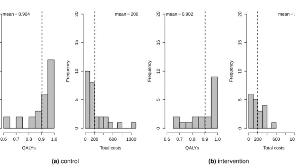
3.2 QALYs and total cost distributions for the control and intervention groups in the MenSS trial. . . 48

3.3 Empirical distributions for the CC and AC baseline utilities and costs in the PBS trial. 51 3.4 QALYs and total cost distributions for the control and intervention groups in the PBS trial. . . 52

4.1 CEPs and CEACs associated with the models fitted to the data of the MenSS study. 62 4.2 EIB and IB distribution associated with the models fitted to the data of the MenSS study. . . 62

4.3 CEPs and CEACs associated with the models fitted to the data of the PBS study. . 65

4.4 CEPs and CEACs associated with the models fitted to the data of the PBS study. . 66

5.1 Joint distribution p(ei, ci), expressed in terms of a marginal distribution for the QALYs and a conditional distribution for the costs. . . 70

(12)

5.3 Posterior predictive QALYs densities for the models fitted to the MenSS trial. . . . 78 5.4 Posterior distributions for the marginal means of the QALYs and cost variables in

the MenSS trial either under a “complete cases” or “all cases” (blue) scenario. . . . 79 5.5 Imputed QALYs in the control and intervention groups based on the models fitted

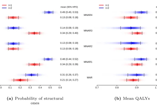
to the data of the MenSS study. . . 80 5.6 Density strip plots for the probability of structural ones and the marginal mean

QALYs under MAR and four alternative MNAR scenarios. . . 81 5.7 EIB and IB distribution associated with the models fitted to the data of the MenSS

study. . . 82 5.8 CEPs and CEACs associated with the Hurdle, Bivariate Normal and Beta-Gamma

models. . . 83 5.9 Posterior predictive cost densities for the models fitted to the PBS trial. . . 86 5.10 Posterior distributions for the marginal means of the QALYs and cost variables in

the PBS trial either under a “complete cases” or “all cases” (blue) scenario. . . 87 5.11 Imputed costs in the control and intervention groups based on the models fitted to

the data of the PBS study. . . 88 5.12 EIB and IB distribution associated with the models fitted to the data of the PBS study. 89 5.13 CEPs (panel a) and CEACs (panel b) associated with the Hurdle (blue dots and

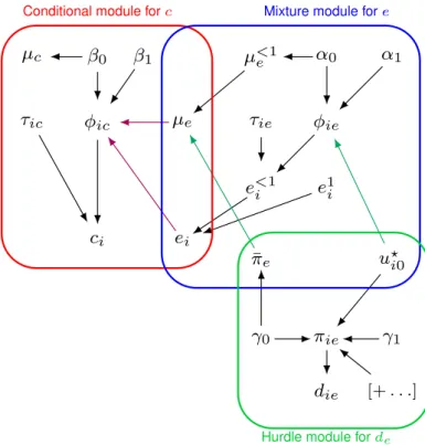
line), Bivariate Normal (red dots and line) and Beta-LogNormal (green dots and line) models. . . 89 6.1 Graphical representation of the four modules related toci0andui0within the

longi-tudinal modelling framework. . . 99 6.2 Densities of the prior distributions of the sensitivity parameters under the three

alternative scenarios:δflat,δskew0andδskew1. . . 101 6.3 Posterior predictive distributions for the pairwise correlation between utilities and

costs variables. . . 104 6.4 Posterior predictive utility and cost densities at each timej= 0,1,2,for the models

fitted to the PBS trial. . . 105 6.5 Observed mean utility and cost profiles in the PBS trial. . . 106 6.6 Posterior means and 95% HPD intervals for the marginal utility and cost means in

each group at each timejin the PBS study across alternative scenarios. . . 107

6.7 Posterior means and 95% HPD intervals for the marginal QALYs and total cost means in each group in the PBS study across alternative scenarios. . . 107 6.8 EIB and IB distribution associated with the models fitted to the data of the PBS study. 108 6.9 CEPs and CEACs associated with with L-CC, L-ALL and the alternative

nonignor-able scenarios. . . 109 6.10 CEPs and CEACs associated with L-CC, CS-ALL, CS-CC, L-ALL andδflat. . . 110 A.1 Graphical representation of the impact of different missingness mechanism on the

(13)

C.1 Diagram representation for the quality score grades based on final scores in three alternative versions for the weight allocation. . . 143 C.2 Mean QALYs and costs estimates derived from three models fitted using the CC or

AC cases of the MenSS trial. . . 146 C.3 Mean QALYs and costs estimates derived from three models fitted using the CC or

AC cases of the MenSS trial. . . 148 C.4 Sensitivity analysis for the choice of the scaling parameterwhen fitting the

Beta-Gamma model to the QALYs and cost data under the “all cases” scenario for the MenSS trial. . . 149 C.5 Sensitivity analysis for the choice of the standard deviation for the distribution of the

structural ones in the QALYs . . . 150 C.6 Mean and 95% credible interval estimates of the expected effectiveness and cost

differentials for the models fitted to the MenSS data under different priors. . . 151 C.7 Mean and 95% credible interval estimates of the expected effectiveness and cost

differentials for the models fitted to the PBS data under different priors. . . 152 C.8 Histograms of the empirical QALYs distributions in the MenSS trial, compared with

those generated from the posterior predictive distributions of the Hurdle Model. . . 153 C.9 Histograms of the proportions of ones in the observed QALYs in the MenSS trial,

compared with those computed from the posterior predictive distributions of the Hurdle Model. . . 154 C.10 Histograms of the empirical cost distributions in the PBS trial, compared with those

generated from the posterior predictive distributions of the Hurdle Model. . . 154 C.11 Histograms of the sample means costs in the PBS trial, compared with those

com-puted from the posterior predictive distributions of the Hurdle Model. . . 155 C.12 Density and cumulative density plots of the empirical cost data in the PBS trial

against the theoretical values obtained from fitting a Gamma or LogNormal distri-bution. . . 156 C.13 Mean and 95% credible interval estimates of the missingness patterns’ probabilities

in the PBS trial. . . 157 C.14 Mean and 95% credible interval estimates of the mean utilities and costs in the PBS

trial. . . 158 C.15 Prior and posterior densities of the distributions of the sensitivity parameters under

the scenarioδflatin the control group . . . 159 C.16 Prior and posterior densities of the distributions of the sensitivity parameters under

the scenarioδskew0in the control group . . . 160 C.17 Prior and posterior densities of the distributions of the sensitivity parameters under

the scenarioδskew1in the control group . . . 161 C.18 Prior and posterior densities of the distributions of the sensitivity parameters under

the scenarioδflatin the intervention group . . . 162 C.19 Prior and posterior densities of the distributions of the sensitivity parameters under

(14)

C.20 Prior and posterior densities of the distributions of the sensitivity parameters under

the scenarioδskew1in the intervention group . . . 164

C.21 EIB and IB distribution associated with the models fitted to the data of the PBS study. 166 C.22 EIB and IB distribution associated with the models fitted to the data of the PBS study. 166 C.23 EIB and IB distribution associated with the models fitted to the data of the PBS study. 167 C.24 CEPs associated with L-CC, L-ALL andδ=0scenarios. . . 167

C.25 CEPs associated with L-CC, L-ALL andδskew0scenarios. . . 168

C.26 CEPs associated with L-CC, L-ALL andδskew1scenarios. . . 168

(15)

Glossary

AC Available Cases

CC Complete Cases

CCA Complete Case Analysis

CEA Cost-Effectiveness Analysis

CEAC Cost-Effectiveness Acceptability Curve

CEP Cost-Effectiveness Plane

CUA Cost Utility Analysis

DIC Deviance Information Criterion

EIB Expected Incremental Benefit

EQ-5D EuroQol-5D

IB Incremental Benefit

ICER Incremental Cost-Effectiveness Ratio

LVCF Last Value Carried Forward

MAR Missing At Random

MCAR Missing Completely At Random

MCMC Markov Chain Monte Carlo

MenSS Men’s Safer Sex

MI Multiple Imputation

MNAR Missing Not At Random

NHS National Health Service

NICE National Institute for Health and Care Excellence

PBS Positive Behaviour Support

QALY Quality Adjusted Life Years

RCT Randomised Controlled Trial

(16)

Research Question and Outline of

the Thesis

Individual-level data in health economic evaluations are generally characterised by some missing outcome values. If these unobserved values are not appropriately handled, they may affect the inferences and possibly mislead the cost-effectiveness assessment. The modelling task is par-ticularly challenging as the problem of handling missingness is often embedded within a more complex framework, where outcome data typically present a series of complexities that need to be simultaneously addressed to avoid biased results.

Trial-based routine analyses do not typically account for all these complexities, are conducted on cross-sectional quantities based only on the complete cases and rarely assess the robustness of the results to different assumptions about the missing values. The failure to appropriately account for the uncertainty generated by missingness may have important consequences on the results and, more importantly, on the approval or reimbursement of new health care technologies. Bayesian methods are well-suited for addressing decision-making problems. By taking a prob-abilistic approach, based on decision rules and available information, they can explicitly account for relevant sources of uncertainty in the decision process and obtain an “optimal” decision out-put. In addition, the flexibility of the Bayesian approach can handle the complexities of the data in a relatively easy way and naturally allows the incorporation and assessment of transparent assumptions about the missing data.

The aim of this research is to develop a full Bayesian approach to handle missingness in health economic evaluations and compare its performance with respect to the standard approach used by practitioners. We address the research question based on three keyobjectives: 1)to review the missingness methods used in trial-based economic evaluations and evaluate the quality of routine analyses with respect to the handling of missing data;2)to identify potential limitations of the standard approach in terms of unrealistic missing data assumptions and provide a Bayesian approach that can improve the current practice and avoid biased results; 3) to develop a full Bayesian approach to handle missingness in a principled way by combining a model for the data and explicit assumptions about the missing values.

The rest of the thesis is structured as follows. Chapter 1 summarises the theoretical back-ground related to the main topics of this thesis. First, we introduce the health economics evalua-tion framework and purpose; then we provide a brief summary of some key concepts of Bayesian analysis and its advantages in dealing with decision-making problems; finally, we present the topic of missing data analysis and we review some of the most popular methods and approaches to handle missingness. Chapter 2 shows the results from a literature review on missingness meth-ods in trial-based analyses and provides recommendations to improve the current practice. In addition, guidelines for assessing the quality of missing data analyses are provided in the form of a structural framework, which is described and applied to the articles studied in the review

(objective1). Chapter 3 presents the two case studies (MenSS and PBS trials) that will be

(17)

routine analyses. Chapter 4 illustrates a pitfall related to the different missing data assumptions associated with alternative implementations of the mean baseline adjustment methods used in routine analyses. Data from both case studies are used to demonstrate the potential bias associ-ated with this method (objective2). Chapter 5 presents a general Bayesian analytic framework that improves the standard approach and leads to more realistic imputations by jointly tackling the typical complexities that affect the data. We demonstrate the benefits and flexibility of our approach on the data from the two case studies (objective2). Chapter 6 proposes a parametric Bayesian longitudinal approach that extends the modelling framework of economic evaluations to handle missingness more efficiently, while incorporating a sensitivity analysis to alternative miss-ingness assumptions. We motivate and apply our approach using the data from the PBS trial

(objective3). Finally, Chapter 7 summarises the main conclusions from this thesis and suggests

(18)

Chapter 1

Background

We first introduce health economic evaluations, the type of data analysed and the decision-making problem involved in the cost-effectiveness assessment. Next, we briefly review some key concepts of Bayesian inference and describe the advantages of using a Bayesian approach to account for multiple forms of uncertainty in economic evaluations. Finally, we present the topic of missing data from a general statistical perspective, review some of the most popular methods used to handle missingness and focus on a principled approach for conducting sensitivity analysis to plausible missingness assumptions.

1.1 Health Economic Evaluation

Economic evaluations are applied in the field of healthcare with the principle aim of improving the economic efficiency of resource allocation, i.e. help maximise benefits from available (and constrained) resources. This has become an increasingly important problem in many countries over the last decades due to a continuous increase in the costs associated with healthcare ser-vices that now affect a great portion of the total economy expenditures (OECD, 2015). Naturally, this is the result of an increase of the average life expectancy and the development of new and more expensive technologies. A major consequence of this process is the need to balance the total healthcare spending, i.e. to define what is the optimum expenditure level and specify how to reach it. In countries where there is a predominant public funding of healthcare, such as the UK, this is typically achieved by defining a governmental health scheme that can provide the highest clinical benefit level for the patients and society, given the availability of limited resources.

In the UK, the National Institute for Health and Care Excellence (NICE) plays an important role with regard to the approval of new healthcare technologies and uses economic evaluations to inform decisions about a wide range of interventions: medical devices, diagnostic technolo-gies, surgical procedures and pharmaceuticals (NICE, 2013). NICE provides evidence-based guidelines on how a particular disease or condition should be treated and assesses whether new treatments provide value for money as they become available in England and Wales (Meltzer, 2001).

The increasing use of economic evaluation for decision-making has placed requirements on the type of evidence and analytic methods to be used in order to define an appropriate framework for the analysis (Sculpher et al., 2005). NICE typically relies on decision models to evaluate the cost-effectiveness of new treatment regimens. These models are based on information collected from the literature, among which a key role is played by Randomised Controlled Trials (RCTs). They provide individual patient data where the randomisation of patients to treatment acts to reduce bias, and therefore can be used to perform head-to-head comparisons in controlled

(19)

envi-ronments. As a result, RCTs are commonly used as a vehicle for economic evaluations. Many funders, such as the UKNational Institute for Health Research Health Technology Assessment Programme, routinely request that assessments of cost effectiveness are incorporated in the de-sign of randomised trials to inform policy makers about the feasibility of extending the treatment to the overall target population.

Economic evaluations can be formally defined as the comparison of alternative options in terms of both theircostsandbenefits (Drummond et al., 2005). The joint consideration of both outcome measures represents a key element in determining whether a new treatment option should be given priority in terms of resource allocation with respect to an alternative. The most popular types of economic evaluation in healthcare areCost-Effectiveness Analysis (CEA) and

Cost-Utility Analysis (CUA), which share a similar rationale but typically differ by the types of measures used to describe the benefits.

In CEA, the benefits of an intervention are measured in terms of a pre-defined unit of health outcome such as lives saved or life years gained and the task of an analyst performing the evalu-ation is to estimate the cost per unit of health outcome achieved, i.e. the cost per life saved. CEA does not permit a direct comparison of costs and benefits across interventions yielding different outcomes (for instance, cases prevented vs. life years gained) but is restricted to the compar-isons of interventions that use the same disease-specific outcome measures. However, health-care providers, such as theNational Health Service(NHS) in the UK, require the comparison of interventions across different disease areas to inform resource allocation and prioritisation deci-sions.

To avoid the problem of non-comparability, benefits in CUA are expressed in terms of utility or quality of life. Among these non-monetary measures, one of the most popular isQuality Adjusted Life Years(QALYs), an index comprising both length and quality of life. Although this has been debated (Mooney, 1989; Neumann and Greenberg, 2009), it is generally assumed that the QALY is a comprehensive measure of health that captures enough aspects of health to be considered an appropriate instrument for measuring outcomes in the field of curative healthcare.

More specifically, QALYs measure the state of health of a person or group in which the ben-efits, in terms of length of life, are adjusted to reflect the quality of life (one QALY is generally associated with one year of life in perfect health). QALYs are calculated by estimating the years of life remaining for a patient following a particular treatment or intervention and weighting each year with a quality-of-life or utility score (see Section 1.2 for more details), which is often measured in terms of the person’s ability to carry out the activities of daily life, and freedom from pain and mental disturbance.

The result of a CUA is usually expressed in terms of total net cost per unit of utility or qual-ity (e.g. cost per QALY gained). As in CEA, the value of measures is still implicitly defined as part of the QALY component but has the general advantage of being used across many different disease areas. This makes CUA very attractive because effectiveness, measured in terms of life expectancy, is a straightforward concept for most clinicians and utilities are a quantitative mea-sure about the strength of patients’ preferences for certain health states. However, issues arise when calculating utility measures due to a variety of available statistical methodologies as well as different types of patients’ data that could be used (Hunter et al., 2015). Although CUA is more resource and time consuming than CEA, it is the recommended analytic framework for economic evaluations in many jurisdictions such as the UK.

Due to an established practice, especially for analyses on individual-level data, practitioners often use the term CEA to also indicate a cost-utility analysis. Throughout this thesis we will focus on trial-based analyses and use the terms economic evaluations, cost-effectiveness analysis and cost-utility analysis interchangeably, as is commonly done.

(20)

1.2 Individual-Level Data

A multivariate outcome constitutes the main focus of economic evaluations: the costs and benefits associated with the treatments under examination. We now present a brief description of how these individual-level variables are typically computed and the features that characterise the data. In a trial setting, e.g. RCTs, health benefit and resource use data are typically collected on each individual in the study (i = 1, . . . , n) at baseline (j = 0) and at successive follow-up times

(j= 1, . . . , J) for each treatment groupt. Data on some baseline demographic variables (e.g. age,

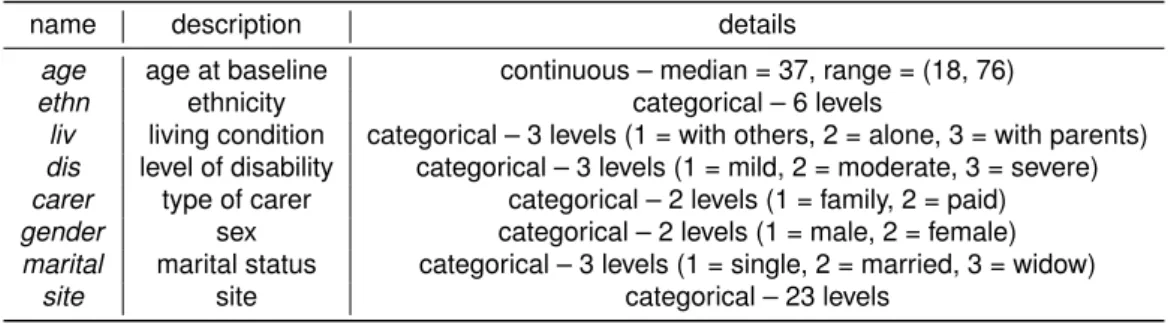
gender, ethnicity, etc.) are also typically collected. Table 1.1 displays an example of a typical trial-based individual level dataset for economic evaluation.

Demographics utility data cost data

Individual t Gender Age . . . u0 u1 . . . uJ c0 c1 . . . cJ

1 1 M 23 . . . 0.32 0.66 . . . 0.44 £103 £241 . . . £80

2 1 M 21 . . . 0.12 0.16 . . . 0.38 £1204 £1808 . . . £877

3 2 F 19 . . . 0.49 0.55 . . . 0.88 £16 £12 . . . £22

4 1 F 20 . . . 0.23 0.37 . . . 0.52 £99 £150 . . . £85 . . . .

Table 1.1:Example of a typical trial-based dataset used in economic evaluations.

Different types of effectiveness or benefit measures can be considered, even though decision-making bodies typically favour outcomes that are comparable across as many different disease areas as possible. Generic preference-based measures ofhealth related quality of lifeare typically used for economic evaluations, and are obtained from short health questionnaires that measure patients’ health and well-being across a number of domains. The questionnaire most favoured in the UK is theEuroQol 5D(EQ-5D,http://euroqol.org) and the variant currently most commonly

used is the 3-level version. The EQ-5D is constructed on the basis of five different domains (mobility, self-care, usual activities, pain and anxiety/depression) for which patients are asked whether they have no, some or extreme problems (three levels), for a total of35 _{= 243}_potential

distinct health states. For example, the health state (11223) is associated with an individual who

reports no problems (level 1) in the mobility and self-care domains, some problems (level 2) in usual activities and pain, and extreme problems (level 3) in anxiety/depression.

Each health state is then associated with a country-specific utility score representing the pref-erences of a sample of the general population for that specific health state. Utility scores are calculated using preference-based algorithms which typically anchor the scores so that a value of

1 corresponds to perfect health and a value of0 is equivalent to the state of death; sometimes,

depending on the specific method used, negative scores are possible, representing states that are theoretically worse than death. For example, in the UK, the utility scores for the EQ-5D 3-level version range from a value of1for perfect health to−0.594, which corresponds to the worst

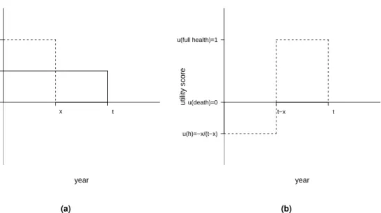
possible health state. NICE’s recommended algorithm to calculate the utilities is the time-trade off (Dolan and Gutex, 1995), in which the utility scores associated with health states considered better or worse than death are valued using different approaches. Figure 1.1 shows how the al-gorithm derives the utility scores associated with an hypothetical impaired health stateh, which is

either valued better (panel a) or worse (panel b) than death.

For an impaired stateh, which is considered better than death (panel a), the respondent faces

a choice between two hypothetical lives: one involvingxyears of healthy life, followed by death

(alternative 1); the other involvingtyears in stateh(wherex≤t), followed by death (alternative

2). If the respondent prefers alternative 2 to alternative 1, x is increased to make alternative

1 more attractive; if the respondent prefers alternative 1 to alternative 2, xis reduced to make

(21)

u(death)=0 u(h)=x/t u(full health)=1 utility score year x t (a) u(h)=−x/(t−x) u(death)=0 u(full health)=1 utility score year t−x t (b)

Figure 1.1:Schematic representation of the time-trade off algorithm to derive the utility scores associated with some impaired health state, which is either valued better (panel a) or worse (panel b) than death.

Legend:himpaired health state,u(h)utility score of stateh,xtime in full health,ttime in stateh.

choose between the two lives. The utility value ofh, i.e.u(h), is calculated according to how much

healthy time the respondent is willing to forgo at this point of indifference, and is given byx/t. If

the statehis considered by the respondent to be worse than death (panel b), the respondent is

presented with a different choice: between a life involvingt−xyears inh, followed byxhealthy

years and then death (alternative 1); and immediate death (alternative 2). The value ofxis varied

until the respondent’s point of indifference is identified, where u(h) = −x/(t −x). Dolan and

Gutex (1995) validated the time-trade off algorithm on a representative sample of the general UK population to derive a preference-based tariff which directly provides the utility scores associated with each of the health states of the EQ-5D questionnaire. For example, using this tariff, the utility score associated with the state (11223) is equal to0.255.

The decision of which types of resource use are included in an economic analysis is usually tailored to the requirements of the decision-makers, i.e. the target audience of the evaluation. For a number of countries, healthcare decision-making bodies only consider healthcare costs when assessing the cost-effectiveness of a new intervention. However, in principle, other costs could be included, e.g. societal costs. In addition, the types of cost and resource data collected can be different (patient questionnaires, clinic records, administrative records), depending on the perspective of the decision-maker.

Aggregate measures of effectiveness (e.g. QALYs) and total costs for each individual and treatment option are typically computed by combining the utilitiesuijt and costscijt collected at each time point into cross-sectional quantities(eit, cit)1as

eit= J X j=1 (uijt+uij−1t) xj 2 and cit= J X j=1 cijt, (1.1) wherexj = Timej −Timej−1

Unit of time is the fraction of the time unit (e.g. 12 months) between consecutive

measurements, e.g.x2= (6 months_{12 months}−3 months)= 0.25. For the utilities, this approach is often referred

to as thearea under the curve(Drummond et al., 2005).

Essentially, QALYs are calculated as a series of preference-weighted health states, where the

(22)

weights (i.e. the utility scores at each time point) reflect the desirability of living in those states. Once the weights are derived, they are multiplied by the time spent in the associated state and these products are then summed to obtain the QALYs. Thus, the QALY values associated with an individual, and their range, depend both on the utility scores at each time pointjand the time

horizonJ considered. For example, given a time duration of 1 year, the QALY value associated

with an individual who has always lived in perfect health (i.e. utility scores of1at each time point

j) is equal to1. However, if a time duration of2years is considered, the QALY value associated

with the same individual living in perfect health throughout this period is equal to2. Similarly, the

QALY value associated with an individual living in the worst possible health state (uj =−0.594 at eachj) is equal to−0.594whenJ = 1year and−1.188 whenJ = 2years. When the QALYs

and total cost outcomes are evaluated over a time period longer than 1 year, their values are

typically discounted using some yearly discount rate r to account for time preferences in the

receipt of costs and benefits, where the value for the discount rate currently recommended by NICE is equal to3.5%(NICE, 2013). Since for both the case studies analysed in this thesis the

time horizon is equal to1 year, the range of the QALYs always coincides with that of the utility

scores, i.e. between−0.594and1, and no discounting is required for both QALYs and total costs.

In general, cost data can vary widely between individuals, are defined on the range[0,∞)and

tend to be positively skewed. The skewness of cost data is typically due to the fact that for many evaluations a smaller number of patients will accrue substantially higher costs compared to other patients. This may be due to, for example, long inpatient stays or expensive interventions. It is also common to observe individuals who are associated with a null cost and that induces a spike at0in the cost distribution.

In the UK, the utility scores for the EQ-5D 3-level version are defined on the range[−0.594,1],

where negative values are associated with health states that are considered worse than death (Dolan and Gutex, 1995). Among the general population, utility data tend to be negatively skewed, with most of the values lying at the higher end of the measurement scale and some observations dis-playing extremely low utility levels. Similarly to the costs, some individuals are typically associated with a perfect health state that induces a spike at1in the utility distribution. Right-skewed

distri-butions of utilities are occasionally observed among certain groups of patients (e.g. terminally ill patients or individuals with chronic conditions) where most of the individuals in the sample report poor health states.

A typical feature of individual-level utility and cost data is that they can be either positively or negatively correlated. The first case may arise, for example, when effective treatments are innovative and are associated with higher unit costs. The second case, instead, may result when more effective treatments reduce total care pathway costs e.g. by reducing hospitalisations, side effects, etc. In addition, when the data are collected from different centres or clusters, utilities and costs can be differently correlated at the individual and cluster level.

This typically occurs in cluster randomised trials, where the unit of randomization is the “clus-ter” – for example, the hospital or primary care physician, not the individual. A cluster design may be chosen because the intervention operates at a group rather than at an individual level (e.g. changing incentives for providers) or if there is a high risk of “contamination” among the individuals within clusters (e.g. evaluating different advertising strategies to encourage smoking cessation). In cluster RCTs, individuals within a cluster are likely to be somewhat similar in their characteristics and the care they receive, and therefore, individual utilities or costs within the same cluster tend to be more homogeneous than those in different clusters (Gomes et al., 2012a). For example, cost data based on process measures such as length of stay, typically have a rela-tively high proportion of the variation at the cluster rather than at the individual level (Campbell et al., 2005). Thus, in cluster RCTs, the size or direction of the correlation may differ according to whether the focus is at the individual or the cluster level (Gomes et al., 2011). For example, within

(23)

clusters, individuals with lower health status may incur higher costs (i.e. at the individual level, there is a strong negative correlation), while clusters that have higher mean costs per patient may have on average higher utilities.

Finally, some observations for either or both outcomes, are almost invariably missing. Reasons for missingness may differ according to the context considered or the individuals’ characteristics (e.g. age, sex, etc.) and outcome values. For example, when data for utilities and costs are derived from similar types of sources throughout the trial, e.g. using self-reported questionnaires, then missingness at a given time typically occurs in both outcomes, e.g. when an individual drops out from the study. However, in trial-based analyses, outcome data may also be derived using different types of sources, e.g. EQ-5D questionnaires for the utilities and a combination of observational datasets and NHS average unit prices for the costs. In this case, reasons and patterns of missing data may be different between utilities and costs and missingness in one outcome may imply or be related to missingness in the other outcome. In addition, when utility and/or cost data for the

i−th individual in the study are not observed at all time points, then(eit, cit)cannot be directly computed as in Equation 1.1 for those subjects and are recorded as missing. When the data are partially-observed or “incomplete”, there are important implications for their analysis that cannot be ignored (we address the implications of missing data analysis in Section 1.5).

1.3 Bayesian Analysis in Economic Evaluation

From the statistical point of view, trial-based CEAs have historically been performed using fre-quentist methods: these include power calculations at the design stage and calculation of p-values and confidence intervals (Briggs and Gray, 1998; Laska et al., 1999; Willan, 2001; Glick, 2011). However, the increasing sophistication of economic evaluations is highlighting the limita-tions of this approach. For example, unlike standard statistical analyses, economic evalualimita-tions do not just focus on estimation (e.g. the computation of point or interval estimation, or hypothesis testing), but are used as a tool to aid decision making (Claxton, 1999). Thus, rather than relying merely on statistical and clinical significance, economic evaluations need to quantify the impact of the uncertainty in the evidence on the entire decision-making process (e.g. to what extent the uncertainty in the estimation of effectiveness of a new intervention affects the decision about whether it is paid for by the public provider). To this aim, much of the recent research has been oriented towards building the economic evaluation on sound statistical decision-theoretic founda-tions (Spiegelhalter et al., 2004; Briggs and Gray, 1999), and increasingly often under a Bayesian statistical approach (O’Hagan and Stevens, 2001; Baio, 2012). In particular, NICE advocates the use of this decision-theoretic framework as a standardised approach in health economic evalua-tions to ensure the comparability of results and the consistency of decision-making (NICE, 2013). Therefore, although alternative approaches to decision-making exist in other application areas, the thesis discusses and focuses on the decision-theoretic approach recommended by NICE, to which all economic evaluations in the UK are expected to adhere.

There are several reasons which make the use of the Bayesian approach in economic evalua-tions particularly appealing. First, Bayesian methods are naturally embedded in the wider scheme of decision theory; by taking a probabilistic approach, based on decision rules and available infor-mation, they can explicitly account for relevant sources of uncertainty in the decision process and obtain an “optimal” course of actions. Second, Bayesian modelling is characterised by extreme flexibility, which allows to account for the typical complexities of the data (e.g. correlation, skew-ness, spikes and missing data) in a relatively easy way. Third, the Bayesian approach naturally allows the incorporation of evidence from different sources (e.g. expert opinion or multiple studies) into the analysis, which may improve the estimation of the quantities of interest compared with

(24)

us-ing the evidence from a sus-ingle source (e.g. a sus-ingle trial). Finally, under the Bayesian approach, it is straightforward to assess and quantify the impact of uncertainty in all inputs of the decision process; this is extremely relevant in economic evaluations as it is a required component in the approval or reimbursement of a new intervention for many decision-making bodies, such as NICE in the UK (Claxton et al., 2005).

We briefly introduce the main aspects of Bayesian inference and focus on how the economic evaluation process is performed within a Bayesian framework. The concepts illustrated in this chapter constitute only a limited insight into the more general and complex Bayesian statistical theory. For a more comprehensive and exhaustive presentation of these topics we refer the reader to Gelman et al. (2013), Jackman (2009) and Lee (2012).

1.3.1 Bayesian Inference and Computation

In contrast with the frequentist approach, which assumes a unique, correct or “true” value of the probability attached to any uncertain event, the Bayesian approach interprets the probability as a “subjective” degree of belief, which depends on the individual whose uncertainty is being expressed and the information available to him/her. Under this perspective, each individual is entitled to his/her own subjective probability, which can be updated according to the evidence that becomes sequentially available.

From a modelling perspective, the Bayesian interpretation of probability allows to make prob-abilistic statements directly on the quantities of interest, i.e. some unobservable feature of the process under study, typically represented by a set of parameters. More specifically, a Bayesian model specifies a full probability distribution to describe uncertainty in terms of the data, which are subject to sampling variability, and unobserved quantities (e.g. parameters or future observa-tions), which are not typically known to the experimenter. As a consequence, probability is used in the Bayesian framework to assess any form of limited knowledge. The experimenter needs to identify a suitable probability distribution to describe the overall uncertainty about the datayand the unknown parametersθ, which we indicate withp(y,θ).

By the basic rules of probability we can re-express this joint distribution as the product of the marginal distribution of the datap(y)and the conditional distribution of the parameters given the

datap(θ|y)or vice versa, i.e.p(y,θ) =p(y)p(θ|y) =p(θ)p(y|θ). From this, we can derive the

fundamental theorem of Bayesian inference known as Bayes theorem:

p(θ|y) = p(y|θ)p(θ)

p(y) (1.2)

The basic idea underlying the theorem is that we can update our level of uncertainty about the pa-rameters before observing the data, expressed through aprior distributionp(θ), with the evidence

from the data, expressed through thelikelihoodp(y|θ), into aposterior distributionp(θ|y). This

allows us to make inference in terms of direct probabilistic statements.

When little information is contained in the prior p(θ), which is then typically referred to as a

diffuse or vague prior, the resulting posterior will be mostly informed by the likelihood. Thus, inference will be numerically similar to that achieved in a frequentist setting, where only informa-tion from the data is considered. However, because of the different assumpinforma-tions underlying the Bayesian and frequentist statistical frameworks, the interpretation of the results between the two approaches remains different.

Alternatively, we can use informativepriors, i.e. distributions that represent some knowledge about the model parameters before observing the data and that, together with the likelihood, drives posterior inferences. The most serious issue with using informative priors is related to the way information is elicited, i.e. brought into the model. More generally, the elicitation process

(25)

implies that the people providing the information to be included in the model (e.g. clinical experts) possess some kind of knowledge or beliefs “in their heads” and it is the analyst task to devise the right kind of questions to “extract” this information from them (O’Hagan et al., 2006).

It is crucial to find an appropriate way to express the external information collected in order to adequately inform the priors on the parameters of interest in the setting analysed. There is a wide literature about the process of eliciting experts probabilities and alternative approaches are available (Stevens and O’Hagan, 2002; Grigore et al., 2016; Mason et al., 2017). Elicited probabilities may suffer from biases and non-coherence in practice, but the goal of the elicitation is to represent the expert knowledge and beliefs as accurately as possible. We will not further cover this subject as it falls outside the focus of this work and we refer to O’Hagan et al. (2006) for a more comprehensive examination on the topic.

A Bayesian analysis can assess the level of uncertainty for any unobserved quantity, be it a parameter or some future observation, given the information from the observed data and model assumptions. For example, it is possible to evaluate probabilistically unobserved datay, assumed˜

to be of the same nature as those already observed, by means of the (posterior)predictive distri-bution

p( ˜y|y) =

Z

p( ˜y|θ)p(θ|y)dθ. (1.3)

The expression indicates that, once the uncertainty regarding the unknown parameters has been integrated out, p( ˜y | y)does not depend on θ anymore and indicates what we know about the distribution of the (future) y. When only prior information is available, we replace p(θ | y)by

p(θ)in Equation 1.3. This yields theprior predictive distributionp( ˜y) = R

p( ˜y | θ)p(θ)dθ, which

corresponds to the denominator of Equation 1.2.

While the posterior distribution might be known in closed form, it is often not analytically tractable. Iterative approximation methods are typically used to approximate the posterior dis-tribution and produce the required inference. Among these, one of the most popular techniques isMonte Carlo Integration(Kroese et al., 2013), which uses a series of random values to numer-ically compute a definite integral. More details on how Monte Carlo integration can be used to derive posterior summaries is available in Appendix A.1.

When the posterior distribution is not available in closed form, a more general class of algo-rithms which can be used to derive posterior inferences is provided byMarkov Chain Monte Carlo

(MCMC) methods (Brooks et al., 2011). MCMC methods are a class of iterative algorithms for sampling from generic probability distributions, which are based on the construction of a Markov chain that converges to the desired target distribution, i.e. the joint posterior distribution of the parameters we are interested in. Provided that some regularity conditions are satisfied (Jackman, 2009; Brooks et al., 2011), after a sufficiently large number of iterations the chain will forget its initial state and will converge to the unique stationary target distribution, which does not depend on time or the initial position.

There are different types of MCMC algorithms. One of the most popular isGibbs sampling (Ge-man and Ge(Ge-man, 1984), which samples sequentially from the full conditional distribution of each parameter or block of parameters. For a detailed presentation of different types of MCMC meth-ods we refer to Brooks et al. (2011). Over time, many software that are specifically designed for the analysis of Bayesian analysis using MCMC techniques have been developed. Perhaps, the software that have most proliferated among applied statisticians are those based on the model de-scription language known asBUGS(Bayesian inference Using Gibbs Sampling; Gilks et al., 1994; Lunn et al., 2012). Some examples are: WinBUGS, and its open source variantOpenBUGS; and JAGS(Just Another Gibbs Sampler; Plummer, 2010). Recently, another probabilistic programming language, calledSTAN(Carpenter et al., 2017), has been developed for conducting Bayesian infer-ence using a specific class of MCMC methods known asHamiltonian Monte Carlo(Brooks et al.,

(26)

2011).

Once the MCMC sampling has successfully been performed, for each parameter of interest we can typically access a vector ofS simulations(θ(1)_{, . . . , θ}(S)₎_{from the posterior distribution. This}

can then be summarised by computing a variety of quantities, such as the posterior mean or me-dian, with uncertainty typically represented via “credible” intervals obtained from the percentiles of the posterior. For example, we can compute the posterior mean E[θ | y]by averaging across

the simulated valuesθ(s)_{or derive an approximate}_95%_{credible interval} _{(CI) using the empirical}

2.5%and97.5%quantiles of the posterior distribution ofθ. A slightly different type of interval is the

95%highest posterior density(HPD) interval. This corresponds to the CI that contains the values

ofθthat are a posteriori more plausible, i.e.p(θ|y)is higher for allθs inside the interval than for

values outside the interval.

Generally speaking, there is no measure that can definitely assess whether the MCMC has converged because the chain will reach the target distribution (forgetting its initial state) only asymptotically. However, some diagnostic measures such as thepotential scale reduction factor

and theeffective sample size(Gelman et al., 2013) may provide some useful insights to detect failures in convergence or high autocorrelation in the MCMC sampler. We do not go further into details about MCMC methods as they are not the main focus of this work, and we refer to Brooks et al. (2011) for a comprehensive text about MCMC methods and inference.

1.3.2 Model Checking

A crucial part of any statistical analysis is assessing the fit of the model. In Bayesian analysis this includes checking for any sensitivity to the choice of the prior in addition to more “standard” checks regarding, for example, residuals and predictions (Gelman et al., 2013). In particular, when comparing models, it can be informative to evaluate their predictive accuracy and perform model selection based on their fit to the data.

A typical approach to assess the predictive accuracy of a Bayesian model usesposterior pre-dictive checks (Gelman et al., 2013). The basic technique is to draw simulated values from the posterior predictive distribution (Equation 1.3), and compare these to the observed data, either graphically or using discrepancy measures. If the model fit is reasonable, then the predictions generated by the model should look similar to the observed data. Different types of graphical as-sessments can be used, including a display of all the data, data summaries or residuals (Gelman et al., 2013). A potential issue with using posterior predictive checks is that, since the data have influenced the estimation of the parameters, they are in fact used twice, i.e. for model fitting and checking. This is not optimal as, in principle, the fit of the models should be evaluated on some external data that were not used for estimation. However, posterior predictive checks can provide useful insights about potential failings of the model, provided that usage is limited to study model adequacy, not for model comparison and inference (Meng, 1994).

Alternative measures of model checking, known asinformation criteria, have been proposed. These measures evaluate the predictive ability of competing models in terms of the accuracy of the models’ predictions based on the observed data and some bias correction terms. For a comprehensive review of different types of criteria we refer to Gelman et al. (2014) and Vehtari et al. (2017). For the analyses in this thesis, we specifically focus on the Deviance Information Criterion (DIC; Spiegelhalter et al., 2002), which is the predictive measure of choice in many Bayesian applications, in part because of its incorporation in the popularBUGSsoftware. A detailed description of how DIC can be computed and the potential pitfalls in its implementation is available in Appendix A.2.

(27)

1.4 Decision Modelling in Economic Evaluation

Health economic evaluations are a typical problem of decision-making under uncertainty. Their main objective is to provide decision-makers with a useful tool that permits the comparison of competing technologies in terms of the benefits they provide and the resource use required to reach these benefits. This leads to the need of some methods to compare alternative options, reflect uncertainty in the conclusions and choose which option should be applied to the whole population, given the available evidence (e.g. coming from a RCT).

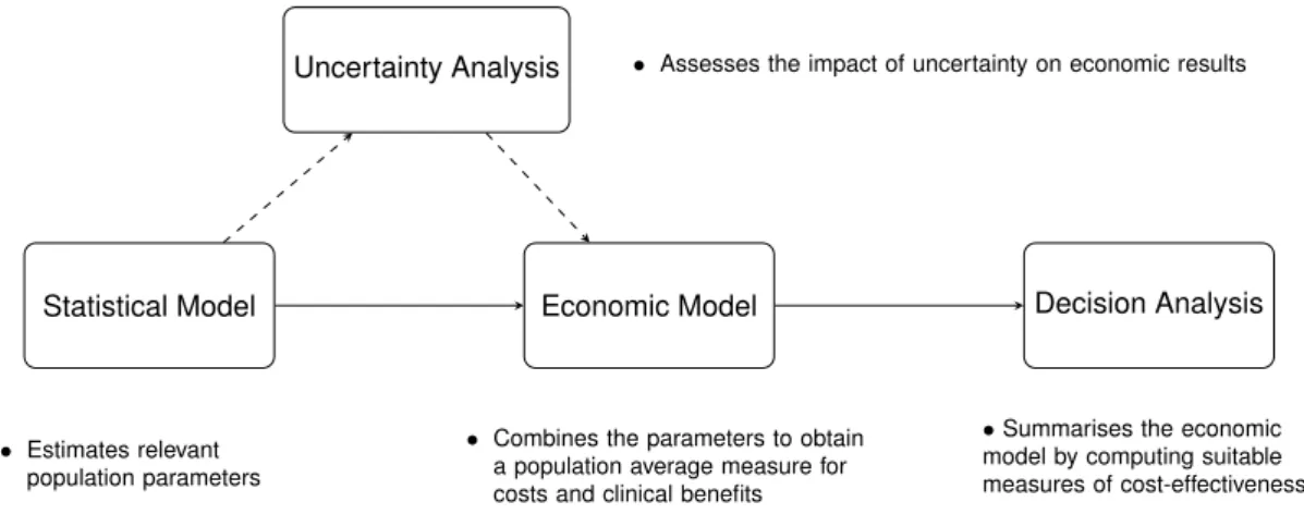
Figure 1.2 graphically represents the general process of doing a Bayesian analysis (with a view of using the results of the model to perform an economic evaluation). Four steps form the process:

Statistical Model. At the beginning of the process a statistical model is used to estimate some

relevant parameters, such as the population mean effectiveness and costs. The type of statistical analysis varies with the nature of the underlying data (e.g. individual level versus aggregated level data).

Economic Model. The estimates from the statistical model are then combined in the economic

model, with the objective of obtaining some relevant population parameters indicating the average benefits and costs for a given intervention in comparison to another one. Depending on the type of available data and statistical model used, this step may simply correspond to using the parameters as derived from the statistical model or it may involve complex combinations thereof (Baio, 2017).

Decision Analysis. Once appropriate outcome measures are obtained from the economic model,

these are used as the basis for the decision analysis, which aims at identifying the optimal intervention that should be applied to the target population by computing suitable measures of “cost-effectiveness".

Uncertainty Analysis. The final aspect is represented by the evaluation of how the uncertainty

(e.g. in parameters or model structure) impacts the final decision outcome and obtain the best course of action given current evidence. However, when the available evidence is limited, it is important to assess the impact of current uncertainty on decision-making.

Statistical Model Economic Model Decision Analysis

Uncertainty Analysis • Assesses the impact of uncertainty on economic results

• Estimates relevant population parameters

• Combines the parameters to obtain a population average measure for costs and clinical benefits

•Summarises the economic

model by computing suitable measures of cost-effectiveness

Figure 1.2: Economic evaluation process. The process is formed by four main steps, represented as rectangles, connected to each other by arrows (indicating the dependency relationships). The flow of the process is indicated by solid arrows, while dashed arrows link the steps subjected to uncertainty assessments. Source: Baio et al. (2017).

The first two steps (Statistical and Economic Model) are related to the construction of appropri-ate models to obtain inferences and their forms mainly depend on the available data and modeller

(28)

approach. Conversely, the last two steps (Decision and Uncertainty Analysis) can be represented in a more standardised way. Specifically, their purpose is to obtain summary CEA measures of interest for decision makers and assess the current level of uncertainty in the decision problem. We now focus on these steps and on the tools typically used to perform their tasks.

1.4.1 Comparing Health Interventions

As discussed earlier, the purpose of economic evaluations is to provide information to decision-makers about the costs and benefits for each treatment under evaluation. Decision analysis has been defined as a systematic approach to decision-making under uncertainty (Raiffa, 1968). In the context of economic evaluation, a decision analytic model uses mathematical relationships to define a series of possible consequences, each associated with specific costs and benefits, for the set of alternative treatments being evaluated. These consequences are then used to inform the best course of action and choose the “optimal” treatment given current evidence, where optimality is defined in decision-theoretic terms (O’Hagan and Stevens, 2001; Briggs et al., 2006; Baio, 2012).

A simple and popular criterion to select an “optimal” strategy in the decision problem of eco-nomic evaluation is themaximisation of the expected utility. The main idea is to choose, among the set of available interventions, the option maximising the probability of the outcome preferred by the decision-maker, i.e. in terms of benefits and costs. When certain conditions are satisfied (Raiffa, 1968; Smiith, 1988), the decision-making can be performed by simply computing an av-erage. In particular, we need to compute for each intervention the expectation of autility function

with respect to both “population” (parameters) and “individual” (sampling) uncertainty/variability. For simplicity, we consider the example where there are only two treatments being compared and generically term the clinical benefits as “effectiveness”. In the following, we indicate the economic outcome variables as(cit, eit), wheret= 1,2denotes the treatment option (e.g. new intervention vs control), and drop the individual indexi to ease notation. Although the definition and type of

the variables(ctandet)may vary depending on the specific conditions considered (e.g. quality of life or survival data), throughout the thesis we assume that they are always expressed in terms of health care costs and QALYs, which are derived from the cost and utility data collected at different time points in the trial using the formulae illustrated in Section 1.2.

As for the type of utility function, health economic evaluations are generally based on theNet monetary Benefit (Stinnett and Mullahy, 1998)

Net Benefit=ket−ct, (1.4)

wherek is a willingness-to-pay parameter used to put the outcomes on the same scale. Note

that the definition provided in Equation 1.4 is based on the standard representation of the net benefit which is typically used in the health economic literature (Claxton, 1999) and that alternative formulations exist (Willan et al., 2004).

The net benefit represents the budget that the decision-maker is willing to invest to increase the benefits by one unit. The main advantage of using the net benefit framework is its fixed form, once

(et, ct)are defined, which provides easy guidance to the evaluation of the interventions. Moreover, Equation 1.4 is linear in(et, ct), which facilitates interpretation and calculation tasks. However, the use of the net benefit presupposes that the decision-maker is risk neutral, which is by no means always appropriate in health policy problems (Koerkamp et al., 2007). For simplicity, we do not focus on this aspect and we assume that the net benefit framework can adequately describe the utility function of the decision-maker, in line with the vast majority of the health economics literature (Briggs, 1999; O’Hagan and Stevens, 2001; Spiegelhalter et al., 2004; Grieve et al.,

(29)

2005; Gomes et al., 2012b; Diaz-Ordaz et al., 2014b; Ng et al., 2016).

Since the net benefit is assumed to be linear in both outcomes, the focus of the analysis can be moved to the estimation of the expected effectiveness and cost quantities, which can then be used in Equation 1.4 to easily derive the expected net benefit associated with each treatment

t. In particular, a statistical model p(et, ct | θ) is typically applied to the cost and effectiveness variables to derive some relevant parameters θ. The model is usually fitted to all treatments under the assumption that some of the parameters θ are shared between treatment groups. In principle, however, it is possible to separately fit a model to each treatment to derive treatment specific estimates for all model parameters, i.e.θ = (θ1, θ2). The interest lies in the population

mean parameters

µet=E[et|θ] and µct=E[ct|θ]. (1.5) The quantitiesµetandµctare then used in assessing the relative cost-effectiveness of the inter-ventions. More specifically, resource allocation decisions are typically based on suitable economic summaries that compare average differences inctandetbetween options. For example, we can re-express the parameters in Equation 1.5 in terms of the population average increments

∆e=E[e|θ2]−E[e|θ1] =µe2−µe1

∆c=E[c|θ2]−E[c|θ1] =µc2−µc1,

(1.6) where ∆e and ∆c are respectively the average increment in the effectiveness and costs from selectingt = 2compared tot = 1. Once the measures in Equation 1.6 are obtained, using the

net benefit as the utility function, it is possible to obtain theIncremental Benefit (IB) of treatment 2 over treatment 1

IB=k∆e−∆c. (1.7)

Notice that, under the Bayesian framework, the quantities(∆e,∆c)in Equation 1.7 are random variables because, while sampling variability is averaged out, these are defined as functions of the parameters of the modelθ = (θ1, θ2). The second layer of uncertainty (i.e. the population,

parameters domain) can be further averaged out. Thus, according to the net benefit framework, decision-making can be effected by considering the so-calledExpected Incremental Benefit (EIB) EIB=E[k∆e−∆c] =kE[∆e]−E[∆c]. (1.8) where, the increment in mean effectiveness and costs (E[∆e],E[∆c]) are actually pure numbers

E[∆e] =e2−e1=E[µe2]−E[µe1]

E[∆c] =c2−c1=E[µc2]−E[µc1].

(1.9) In particular,c2ande2are the population averages of cost and benefit measures for the reference

treatment, to be assessed against those of the comparator (c1, e1). The quantities in Equation 1.8

and Equation 1.9, in turn, can be used to compute the Incremental Cost-Effectiveness Ratio

(ICER), defined as

ICER= E[∆c]

E[∆e]

. (1.10)

The ICER represents the cost per incremental unit of effectiveness (e.g. cost per QALY gained) and provides a ratio summary of the additional cost and benefit that result from one option com-pared to another. From Equation 1.8 and Equation 1.10, we see that when EIB > 0 and so

k > ICER, then t = 2 is the optimal treatment (associated with the highest expected utility).

Thus, decision-making can be equivalently effected by comparing the ICER to the willingness-to-pay threshold.

(30)

1.4.2 Cost-Effectiveness Assessment

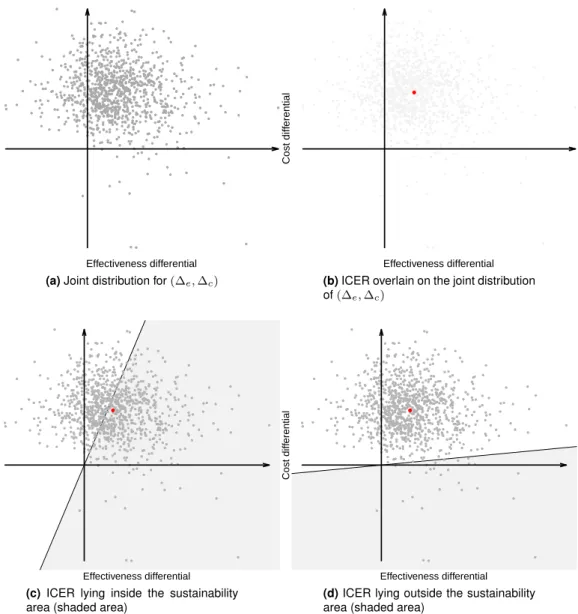
The two layers of uncertainty underlying the decision-making process, as well as the relation-ships between benefits and costs, can be best appreciated through the inspection of the Cost-Effectiveness Plane (CEP; see Black, 1990; Briggs and Gray, 1999; Baio, 2012), shown in Fig-ure 1.3 which is taken from Baio (2012).

Effectiveness differential

Cost diff

erential

(a)Joint distribution for(∆e,∆c)

Cost diff

erential

(b)ICER overlain on the joint distribution

of(∆e,∆c)

Cost diff

erential

(c)ICER lying inside the sustainability

area (shaded area)