Three Essays on Labor Supply

(1)

Three Essays on Labor

Supply

Inaugural-Dissertation zur Erlangung des akademischen Grades eines

Doktors der Wirtschaftswissenschaft des Fachbereichs

Wirtschaftswissenschaft der

Freien Universität Berlin

vorgelegt von Sascha Drahs, M. Sc.

geboren in Berlin

(2)

Gedruckt mit der Genehmigung des Fachbereichs Wirtschaftswissenschaft der Freien Universität Berlin

Erstgutachter: Prof. Dr. Peter Haan

Zweitgutachter: Prof. Georg Weizsäcker, Ph.D. Tag der Disputation: 13. Juni 2018

(3)

Erklärung über Zusammenarbeit mit Koautoren und Vorveröffentlichungen

Die Dissertation ist in drei Kapitel gegliedert. Kapitel 1 und 2 wurden unter meiner alleinigen Autorenschaft verfasst. Bei Kapitel 3 handelt es sich um eine gemeinschaftliche Arbeit von Dr. Amelie Schiprowski, Luke Haywood, Ph. D., und mir.

Kapitel 3 ist bereits als Diskussionspapier unter folgendem Titel erschienen: Sascha Drahs, L. Haywood und A. Schiprowski, „Job Search with Subjective Wage Expectations“, Discussion Paper No. 1725, DIW Berlin, 2018; Discussion Paper No. 75, SFB TRR 190, 2018.

(4)

(5)

3 Job Search with Subjective Expectations 113 3.1 Model . . . 115 3.2 Data . . . 119 3.3 Descriptive Evidence . . . 121 3.4 Structural Estimation . . . 127 3.4.1 Likelihood Function . . . 127 3.4.2 Econometric Specification . . . 128 3.4.3 Identification . . . 129 3.5 Estimation Results . . . 130 3.5.1 Parameter Estimates. . . 130 3.5.2 Model Fit . . . 131

3.5.3 The Effects of Wage Optimism on Job Finding . . . 131

3.6 Conclusion . . . 139

Appendices 141 3.A Gross-Net Conversion . . . 141

3.B Additional Descriptive Evidence. . . 142

(7)

CONTENTS 7

General Conclusion 149

Summary 161

English . . . 161

(8)

(9)

List of Tables

1.1 Summary Statistics of Estimation Sample . . . 30

1.2 Observed Choice Combinations. . . 31

1.3 Estimated Parameters of Utility Function . . . 37

1.4 Estimated Parameters of Wage Equation. . . 38

1.5 Parameter Estimates of Labor Market Shocks . . . 39

1.6 The Effect of Parental Leave Policies on Fertility Rates by Age. . . 50

1.7 Employment Effects: Reform at Age 20 . . . 57

1.10 The Effect of Parental Leave Policies on Employment Rates by Number of Children: Reform at Age 20 . . . 59

1.B.1 Education (ISCED-97) . . . 63

1.B.2 Observed Births by Birth Parity and Survey Year . . . 64

1.B.3 Full-Time and Part-Time Labor Market Experience . . . 65

1.B.4 Contract Term . . . 66

1.B.5 Reasons for Job Change. . . 67

1.B.6 Partnership Status . . . 67

1.B.7 Logistic Regression for Presence of Partner . . . 68

1.B.8 Linear Regression for Partner Income . . . 69

1.B.9 Distribution of Employment Status . . . 70

1.B.10 Distribution of Weekly Hours of Work by Work Category . . . 70

1.B.11 Age at Labor Market Entry by Education Group . . . 71

2.1 Transition Probabilities for Full-Time Employees . . . 84

2.1 Effect Heterogeneity by Age . . . 98

2.A.1 Reform Effect on Employment and Part-Time Work for Different Firm Sizes104 2.A.2 Reform Effect on Part-time Work for Firm Stayers . . . 105

2.A.3 Effects on Employment and Part-Time Work over 2-Year Horizon . . . 106

2.A.4 Effects on Part-Time Work (Stayers) over 2-Year Horizon. . . 107

2.A.5 Effect Heterogeneity by Age for Stayers . . . 108

(10)

3.1 Summary Statistics . . . 121

3.1 Parameter Estimates . . . 132

3.2 Effects of Information Treatment. . . 136

3.3 Effects of Information Treatment: Robustness . . . 138

3.B.1 Wage Optimism and Individual Characteristics . . . 144

3.C.1 Parameter Estimates: Lower Bound Discount Factor (r=0.01) . . . 146

(11)

List of Figures

1.1 Distribution of Part-Time and Full-Time Work over Age . . . 32

1.2 Family Dynamics over the Life-Cycle . . . 33

1.3 Job Risks over the Life-Cycle . . . 34

1.4 In-Sample Fit for Employment Probabilities . . . 41

1.5 In-Sample Fit for the Probability of Giving Birth to a Child by Age . . . 42

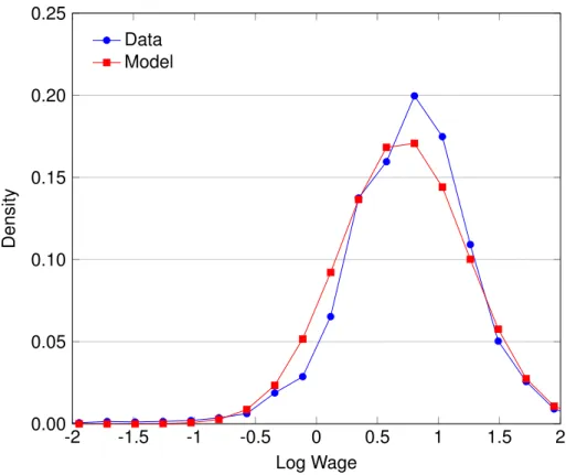
1.6 In-Sample Fit for the Distribution of Wages . . . 43

1.7 Simulated Hazard Rate for Parental-Leave Durations: Reform at Age 20 . 46 1.8 Simulated Hazard Rate for Parental-Leave Durations: Reform at Age 30 . 47 1.9 Simulated Hazard Rate for Parental-Leave Durations: Reform at Age 40 . 49 1.10 Employment Effects for Reform at Age 20 . . . 54

1.11 Employment Effects for Reform at Age 30 . . . 55

1.12 Employment Effects for Reform at Age 40 . . . 56

1.B.1 Gross Wage Distribution . . . 65

1.B.2 Fit of Partner Income Regression . . . 69

2.1 Prevalence of Part-Time Work Among Female Employees . . . 82

2.1 Unconditional Time Trends for Treatment and Control Group . . . 91

2.2 Conditional Pre-Trends for Treatment and Control Group . . . 92

2.1 Baseline . . . 95

2.2 Effects for Age 50–65 . . . 97

2.3 Effects Over 2 Years . . . 99

2.B.1 Part-Time Work Among Female Employees Over Time . . . 109

2.B.2 Effects for Age 20–34 . . . 110

2.B.3 Effects for Age 35–49 . . . 111

3.1 Re-Employment Log Wage (Gross) . . . 122

3.2 Deciles of Re-Employment Log Wage (Gross) . . . 122

3.3 Re-Employment Minus Pre-Unemployment Log Wage (Gross) . . . 123

3.4 Initial Wage Expectation over Pre-Unemployment Wage (Net) . . . 124

3.5 Re-Employment Wage over Wage Expectation (Net) . . . 125

3.6 Subjective Wage Expectations (Net), by Week of Interview . . . 126 11

(12)

3.7 Net Wage Expectation in Wave 1 over Net Wage Expectation in Wave 2 . 127

3.1 Fit of Job Finding Hazard . . . 133

3.2 Fit of Re-Employment Wages . . . 133

3.3 Fit of Subjective Wage Expectations . . . 134

3.4 Simulation: Effect of Information Provision and Search Cost Reduction . 135 3.5 Simulation: Effect of Information Provision for Different Discount Factors . 139 3.A.1 Pre-Unemployment Wages: Gross, Predicted Net and Net . . . 142

3.B.1 Re-Employment Log Wage (Net) . . . 143

3.B.2 Deciles of Re-Employment Log Wage (Net) . . . 143

(13)

Introduction

Until the visionary age of robots will have fully arrived, the production of goods and ser-vices will demand human work, most of which will be traded in the labor market. In 2017, 44 million employees in Germany supplied a total amount of 51 billion hours of work to produce goods and services worth 3.1 trillione1. This is what makes the labor market a central institution for the productive capacity of our society. Consequently, the importance of the labor market in politics and media seems unchallenged by any other market: next to output growth and inflation, it is usually the unemployment rate by which we judge the state of the economy. Still, one may argue: isn’t the supply of energy or the price of computers essential for production, too?2 _{What is it, then, that makes the labor market}

so unique?

In light of the topic of this dissertation, I would like to give the following answer: it is the importance of work for our personal lives. Most people find themselves to participate in the labor market at some point in their lives, and in many cases spend a significant part of their lifetime at the workplace. Work means more than trading leisure for consumption; the possibility of selling one’s skills and work hours to the market provides the foundation for sustaining a standard of living, social status, and providing for one’s children. Because conditions in the labor market have such far-reaching consequences in so many domains of life, understanding and improving these conditions is a rewarding goal.

In the most stylized version of the neoclassical model, the labor supply choice entails an optimal trade-off between leisure and consumption. To analyze the effects of labor market conditions or institutions on individual labor supply decisions, this framework – although true at a sufficient level of abstraction – does not possess enough depth of detail. In this dissertation, I analyze, chapter by chapter, three core aspects of individual labor supply, where each aspect will emphasize a concretization of the standard framework.

I start out from the origin of individual labor supply decisions: the private domain, or more succinctly, the family. Chapter 1 analyzes the labor supply decisions of women, taking into account family planning. The importance of the childbearing decision is evi-dent from the fact that female labor supply declines sharply with the presence of children. Hence, the leisure-consumption trade-off of mothers is structurally different from that of

1_Destatis _[₂₀₁₈_{], GDP as of 2016.}

2_{In 2017, each produced}_e_{’s worth used 59 seconds of work [}_Destatis_,₂₀₁₈_{, own calculations], but 89}

grams of oil equivalent of energy [The World Bank Group,2018,OECD,2018, own calculations].

(14)

childless women. In the first chapter, I add two central ingredients to the model of labor supply – unemployment and dynamics – to analyze how parental leave policies can affect female labor supply and fertility. The presence of unemployment changes the whole game of labor supply: a job becomes a valuable asset, and leaving one’s job to take care of children becomes a risky undertaking. As I show in the empirical analysis, this risk leaps far into the most private domain of family formation when women who work refrain from having children. Moreover, I argue that parental leave legislation provides policy makers with a powerful tool to cushion these adverse effects of job risk on fertility. The second key ingredient in a model of labor supply is dynamic optimization. The dynamic structure of the model presented in this chapter is nowadays a standard way to think about labor supply (and most other economic decisions), because economic actions such as working or family planning are taken under the deliberation of their future consequences.

In Chapter 2, it is taken as given that individuals have made up their minds about their preferred amount of labor supply. As in the preceding chapter, a distinction is made between non-work, part-time, or full-time work3_{, allowing for the empirically relevant}

dis-tinction between the extensive (participation) and the intensive (hours per week) decision margin. The goal of the second chapter is to shed light on the consequences for employ-ees’ labor supply when transitions between full-time and part-time work are not feasible. Looking at female employees in full-time jobs, I analyze the effects of a legal reform mak-ing it easier for employees of medium-sized and large firms to reduce their weekly work hours. Using a quasi-experimental research design, I show that women above the age of 50 reacted strongly to the reform by reducing their hours and leaving their jobs less often. Like in Chapter 1, it is again the private domain which helps to explain the age pattern in labor supply adjustment, as women often take care of own or in-law parents later in their working lives. In analogy to the fertility case, I find that the government can change the legal rules so as to alleviate a conflict between career and private life.

In the final chapter of my dissertation, I broaden the perspective on labor supply by analyzing the search effort of the unemployed.4 _{As prolonged unemployment persists}

to be a pervasive and costly feature of labor markets, most advanced economies have adopted some kind of search assistance. In Chapter 3, my coauthors and I introduce sub-jective expectations as a new ingredient to the analysis of unemployment. Without further mentioning, the analysis in Chapter 1 and 2 assumed that economic agents base their decisions on realistic expectations of the future. We show this is not true of expectations of future wages; using the framework of a dynamic search model, we find that job seekers are optimistic about their future wage offers, which causes them to be unemployed longer than necessary. We suggest information provision as an innovative and cheap tool in job search assistance.

3_{That is, I have discretized the continuous hours-of-work choice into three broad categories.}

4_{The decision to search harder implies finding work earlier and thus increases labor supply in expectation.}

This, in turn, implies frictional unemployment to decline and the aggreate employment level to rise [e.g., Pissarides,2000].

(15)

LIST OF FIGURES 15 As I have laid out above, the three chapters of my dissertation exemplify the policy-relevance of labor supply in three important contexts: the family, the workplace, and in unemployment. For completeness, I should comment on the relationship between labor supply and labor demand (i.e., firm behavior), or labor market equilibrium. Throughout the analysis, I have analyzed individual behaviorceteris paribus, i.e. under the assumption that firm behavior remain unchanged. This approach has both advantages and disad-vantages. First, the motivating reason for abstracting from firm behavior is a trade-off between detail and comprehensiveness: the detailed insights from any of the three chap-ters of this dissertation could not have been gained without the simplifying assumption of exogenous labor demand. Second, the downside to the partial analysis presented here clearly is its agnosticism about equilibrium policy effects. To the policy maker, this may seem like only half of the analysis – and I agree: the analysis of firm’s responses to changes in worker behavior may proceed in the same (partial) manner. Moreover, I think that the combination of credible “partial” evidence and a battery of plausible scenarios of firm response can be a better guide for policy than an equilibrium analysis that is based on too many far-fetched assumptions.

(16)

(17)

Chapter 1 The Effects of Parental Leave

Policies in Labor Markets with

Search Frictions

Parental leave policies contain two key components. First, parental leave job protection reduces the risk of involuntary unemployment for parents after taking parental leave; sec-ond, parental leave benefits help to reduce financial hardships during parental leaves. The goals of these policies are to increase both fertility and female labor supply.

However, there may be a target conflict between these policy goals, and assessing the impact of parental leave policies on both fertility and female labor supply is crucial in designing effective policies. Lalive et al.[2013] show that parental leave job protection and benefits provide incentconsideredives to take parental leave and return within the legal time frame. Since the fertility and the labor supply margin are innately connected, it is interesting to ask what consequences these policies have on fertility. To answer this question, I stress the importance of unemployment risk: in labor markets with search frictions1_{, parental leave policies affect female labor supply by providing additional job}

se-curity and financial support. By the same token, fertility decisions might be affected when these policies improve the situation of parents. In addition to evaluating the trade-off between fertility and labor supply effects, learning about the underlying economic mech-anisms is necessary to understand how job protection and benefits interact to influence both outcomes.

I develop a dynamic discrete choice model of female labor supply and fertility similar toAdda et al. [2017] to evaluate parental leave policies based on longitudinal German micro data. In each time period, women face a joint decision of fertility and hours of work, provided in three broad hours-of-work categories. In each period, income is earned and labor market experience increases wages through a Mincer wage equation. Net incomes

1_{The term search friction denotes the fact that finding a job is not guaranteed to the job seeker.}

(18)

are determined under consideration of taxes and social security payments, unemploy-ment and child benefits using a microsimulation model. Women may be labor market rationed in the sense that no job offer is available. This is modeled by a pair of employ-ment shocks – one for job loss and one for job finding. Importantly, job loss and job finding probabilities depend on labor market experience just like wages do. Moreover, I distinguish between fixed-term and permanent employment contracts; a labor market shock governs period-to-period transitions from fixed-term to permanent work contracts.

To quantify the effect of parental leave policies on fertility and female labor supply, I simulated counter-factual remaining life-cycles for samples of women affected by parental leave reforms at ages 20, 30 and 40. I consider a reduction of the parental leave job protection period from 3 to 2 years and an extension of the parental leave benefit period from 1 to 2 years, and consider the effects on parental leave hazard rates, age-specific and total remaining fertility rates, the employment rate and the part-time share among female employees.

I find that a reduction in job protection decreases remaining fertility by 4.1 % for the sample affected at age 20, and an extension of benefits increases fertility by 4.7 %. Life-cycle employment effects are rather small and seem to be dominated by indirect effects coming though changes in fertility. Effects on the employment rate are not persistent but effects on the part-time share among female employees are. I conclude that reform ef-fects on parental leave durations tend to overestimate the employment efef-fects of parental leave reforms. On the other hand, usually unobserved effects on total remaining fertility rates seem to be positive for both considered policies.

The paper contributes to at least three strands of literature. First, it adds to the large body of research on the economic determinants of fertility [see Hotz et al., 1997, for a survey]. A recent series of papers have been looking at the causal effect of exogenous unemployment shocks on fertility. Using evidence from plant closures in Austria,Del Bono et al. [2012] found that experiencing a job loss reduces subsequent fertility. Del Bono et al.[2015] extended this analysis and found that the fertility effect of job loss incidence remains even after separately controlling for a subsequent unemployment status. Using data from plant closures in Finland,Huttunen and Kellokumpu[2016] showed a negative fertility effect for women who have lost their job, and no effect for women whose partner has experienced a job loss. One can conclude from these studies that women’s own employment prospects matter for their childbearing decisions, and that adverse labor market shocks translate into lower subsequent childbearing. Using German survey data, women who perceive a high risk of becoming unemployed have been shown to have a reduced hazard rate of having a next child [Kreyenfeld,2010,Hofmann and Hohmeyer,

2013]. Moreover, women who lose their job during recessions display a more pronounced reduction in subsequent fertility [Hofmann et al.,2017]. These findings further highlight the importance of labor market search frictions for the childbearing decision. The dynamic structural model in this paper features job risk prominently: the future risk of involuntary

(19)

19 unemployment is taken into account when the childbearing decision is made. Therefore, the important empirical relationship between unemployment risk and fertility is considered in the evaluation of parental leave policies.

In the last decades, there has been a growing interest in the evaluation of parental leave policies. A number of studies have used quasi-experimental methods to analyze the fertility and labor supply effects of parental leave policies exploiting temporal variation of benefits and job protection policies. The literature documents strong positive effects of financial incentives and parental leave job protection periods on the duration of the paren-tal leave:Spiess and Wrohlich[2008] performed an ex-ante policy simulation of a German parental leave benefit reform, which showed that front-loading parental leave benefits re-duces the average parental leave duration. Wrohlich et al. [2012] andKluve and Tamm

[2013] confirmed this prediction ex-post. Using several reforms of the parental leave benefit duration and job protection period in Switzerland, Lalive and Zweimüller [2009] showed that increasing the entitlement period for both benefits and job protection for a current child reduces subsequent employment of mothers. In line with this,Schönberg and Ludsteck[2014] found that several extensions of the parental leave job protection pe-riod in Germany have increased average parental leave durations of mothers. Findings on fertility effects are more sparse but generally positive. Lalive and Zweimüller [2009] showed in the Swiss context that extensions of the length of the parental leave job pro-tection and benefit period for a current child have a positive effect on the probability to have a next child. Using a similar approach with data from Germany,Cygan-Rehm[2016] showed that reducing parental leave benefit payments for the current child reduced the probability to have a next child. Directly looking at short-term birth rates,Raute [2017] exploited a parental leave benefit reform in Germany and found that increasing benefits had positive fertility effects, which are more pronounced for women being older than 35. Thus, existing studies have found compelling evidence of the effectiveness of parental leave policies on both fertility and female labor supply. These findings are in line with the economic model of female labor supply and fertility presented in this paper. However, conventional reform evaluations face limitations in analyzing the effects of parental leave policies on first-birth hazards and lifetime completed fertility rates: available reforms are invariably only sharp at the birth date of the child, such that women in the control group will move into the treatment group as time progresses. This challenge is overcome by using the structural modeling approach in this paper. I simulate counter-factual parental leave reforms to assess a causal effect of parental leave on first-birth hazards, completed fertility rates, and life-cycle female labor supply.

Finally, the paper adds to the literature on structural models of female labor supply and fertility. Starting withHeckman and Macurdy’s [1980] analysis of female labor supply under certainty, a vast literature have used dynamic structural models to answer ques-tions relating to female labor supply. Wolpin [1984] analyzed female life-cycle fertility using a dynamic discrete choice model. Francesconi [2002] estimated a joint model of

(20)

female labor supply and fertility under earnings uncertainty.Adda et al.[2017] estimated a dynamic discrete choice model of female labor supply and fertility with search frictions and occupational choice. They found that a large part of the lifetime income losses from having children are due to occupational sorting. Moreover, they evaluate the effects of a monetary child benefit to find that life-cycle employment outcomes and completed fertil-ity are only mildly affected by such a reform when long-term adjustments are taken into account. Lalive et al.[2013] revisited the reduced-form findings ofLalive and Zweim¨uller

[2009] to show that parental leave job protection and benefits have their strongest impact when used together. My approach extends their analysis by adding a child-bearing deci-sion in a dynamic discrete choice model. This allows me to identify important trade-offs between fertility and labor supply effects of parental leave policies. I stress the impor-tance of job risk by modeling a detailed process for the risk of job loss and the chance of job finding and making a distinction between fixed-term and permanent work contracts. I identify processes for the various labor market shocks using detailed survey information from the German Socio-economic Panel (GSOEP).

The next section provides an outline of the benefits and job protection policies in Ger-many. This will give an insight into the important economic considerations in the timing of childbirth, parental leave, and life-cycle labor supply. Following next, I propose a dynamic discrete choice model of female labor supply and fertility (Section1.2). Afterwards, I dis-cuss the micro data used for the empirical analysis, which is retrieved from the GSOEP (Section1.3). I then describe the estimation method and identification of the labor market frictions (Section1.4). Estimation results ans poicy simulations are presented in Sections

1.5-1.6. Section1.7concludes.

1.1 Institutions

Similar to other countries, parental leave policies in Germany consist of two parts: a parental leave benefit payment (benefits) and the parental leave job protection (job pro-tection).

Parental Leave Benefit. The parental leave benefit2_{is a wage replacement parents can}

receive for up to twelve months following the birth of a child. In 2007 it replaced the prior means-tested benefits by an earnings-related payment: for up to 12 months following childbirth, parents on parental leave receive 65 % of their previous year’s net earnings as a wage replacement in the baseline scenario. If parents choose to work part-time while on parental leave, net income from part-time work is deducted from the benefits amount. Moreover, a minimum amount of 300 Euro is paid for low-income earners, and the ceiling amount for the parental leave benefit payout is 1,800 Euro. In addition to that, some

(21)

1.1. INSTITUTIONS 21 special provisions apply. Most importantly, parents who choose to share parental leave months between partners are eligible for two extra months of benefit payments.

Parental leave job protection. Contrary to benefits, parental leave job protection3

con-stitutes an employee right for parents who are in an employment relationship at the time of childbirth. Within the first three years following childbirth, each parent has the right to reduce work hours or interrupt employment altogether without being at risk of being displaced. Thus, parents who wish or need to take (full-time) care of a newborn can do so flexibly without having to abandon their work position. Therefore, this type of policy is often seen as a means to foster mothers’ labor force attachment. On the other hand, eligibility for job protection is not universal: the work contract is only protected if it does not expire during the parental leave. As temporary contracts are common especially for labor market entrants, a substantial fraction of parents can not fully benefit from the job protection policy.

Fertility and Labor Supply Effects. It is easily seen that both benefits and job protec-tion policies make it easier to take some time off after childbirth for previously employed mothers. Moreover, the time limited nature of these policies provides incentives for the timing of return to work. All else being equal, benefits make the first year of parental leave financially more attractive than parental leave in any other year. Somewhat distinctly, job protection induces a sharp decrease in the value of returning to work right at job protec-tion exhausprotec-tion. For an in-depth discussion of the economic incentives of both policies in a labor supply framework with unemployment risk, seeLalive et al. [2013]. The central labor market implication of parental leave job protection is that labor force attachment of mothers is strengthened, while parental leave benefits reduce the employment rate within the benefit period.

Fertility effects of parental leave policies are ambiguous. On the one hand, the ad-ditional job security and benefit payments increase the value of having a child, with a positive effect on fertility. Parental leave policies, on the other hand, are conditional on labor market aspects such as the wage and the duration of the job contract. When ad-ditional labor market experience is expected to lead to higher benefit payments and a longer effective period of parental leave job protection, then deferring the next childbirth might be optimal. This opposing effect on fertility may be called entitlement effect in anal-ogy to the effect of unemployment benefits on labor supply [see, e.g.Hamermesh,1979], and renders the total fertility effect theoretically ambiguous.

Finally, higher fertility might decrease the overall level of labor supply when there is a complementarity between the number of (small) children and the amount of non-market-work time. This means that a positive fertility effect of parental leave policies might lead

(22)

to a lower participation rate and a higher part-time share. This effect partially offsets any positive effect of these policies on the labor force attachment of women.

In the next section, I will outline the dynamic discrete choice model of female labor supply and fertility, which I will then use to analyze these mechanisms and the role that parental leave policies play in this context.

1.2 Model

To analyze the incentives provided by parental leave policies, I employ a dynamic discrete choice model of female labor supply and fertility. Individuals are assumed to derive utility from consumption, leisure, and from the presence of children. Hence, they choose an optimal amount of hours worked and an optimal number (and birth time) of children in each period of time. Furthermore, individuals are forward looking and foresee that labor supply has a positive externality on wages in future periods of time. Thus, there is a career rationale that also affects the timing of children. For example, when complementarities exist between children and consumption, women may choose to defer child bearing until a higher wage level is attained. Moreover, labor market frictions exist that pose the threat of involuntary unemployment. The risk of unemployment is also affected by labor market experience, providing an additional career incentive to individuals. Finally, jobs may be of a temporary nature at first, with a period-by-period chance of conversion to a permanent contract with associated lower risk of job loss.

This economic framework captures the policy incentives outlined in Section 1.1. In particular, parental leave benefits will lead to postponements of births for individuals with low wages. Likewise, parental leave job protection will induce postponements of births for individuals with temporary work contracts.

1.2.1 Utility and Income

Since parental leave policies have their strongest impact on the labor supply of women before childbearing age and until a few years after children have been born, I restrict the model’s time horizon to the end of the fertile period at ageT1 = 45. The life-cycle starts after completion of education at T0_{. For simplicity, I do not make individual subscripts}

explicit.

The model focuses on the economic determinants of women’s fertility and labor supply choices. To this end, many non-economic factors and private circumstances are not explicitly modeled. Note that this does not imply that choices are made independently of such private circumstances, but that they rather add to the set of unobserved choice characteristics that affect choice through a random utility component.

At each aget, t =T0, . . . , T1, a simultaneous joint decision on the number of hours workedxw_t 2 {N W, P T, F T}and conception of a childxc_t 2 {C, N C}is made such that

(23)

1.2. MODEL 23 Xt ⌘ [xW_t , xC_t ]. Individuals can supply hours of work in three broad categories: full-time (F T), part-time (P T), and non-work (N W). The child decision is binary, conception being denoted byCand non-conception byN C. I define indicator variablesf tt,ptt, and conceivetfor convenience.

Denote bySt ⌘[xwt 1, edut, expert, permt, jprot, nct, act, ht]the state variables of the decision maker (individual) at aget. The state space consists of the following elements:

• labor supply in t 1xw_t ₁ • educationedut2{1,2,3}

• labor market experienceexpert2[0, T1 T0]⇢R • permanent work contract int 1permt2{0,1} • parental leave job protection int 1jprot2{0,1} • number of childrennct2{0,1,2,3}

• inverse age of youngest childact2{0,1,1₂,1₃, . . . ,₁₉1} • presence of a partnerht2{0,1}

where labor market experience is defined as the cumulative number of years worked, with part-time experience being downward adjusted by a factor of 0.5 to account for working hours4_{. Furthermore,}_ac

tis defined as ₁₊_{age of youngest child at age}1 _t andact = 0whennct = 0.

Instantaneous utility Given the state variables and choices, an individual’s instanta-neous utility at agethas the following mixed-CRRA linear form:

ut= ˜ ct1 ⌘ 1 1 ⌘ exp ↵ 0 ct+↵1c,nc·nct +. . . ↵0_pt_·ptt+↵0f t·f tt+. . . ↵0_nc(edut)·nct+↵_nc0 2(edut)·nc2_t/100 +. . .

↵1_ac,t·act·_t˜₍_edut_{) +}_↵1

ac,t2·act·t˜(edut)2/100 +. . .

⇥ ↵1_nc,pt·nct+↵1ac,pt·act ⇤ ·ptt+. . . ⇥ ↵1_{nc,f t}_·nct+↵1ac,f t·act ⇤ ·f tt+. . . ✏u_t, (1.1)

where✏u_t is an i.i.d. type-1 extreme value distributed random utility shock capturing un-observed choice characteristics. ⌘ denotes the coefficient of relative risk aversion, with

4_{This adjustment reflects the relation of mean hours of work in full-time and part-time jobs, as shown in}

(24)

⌘ 6= 15, andct˜ ⌘ p ct

1+ht+nct is the per-capita consumption according to an equivalence scale, depending on the presence of a husband. The second term in (1.1) captures the overall consumption weight and a complementarity between consumption and the number of children. The following two lines reflect baseline preferences for non-market-work time, and a quadratic preference for the overall number of children. To capture age-dependent preferences for fertility, I assume that mothers have age-dependent pref-erences for the presence of young children. This is captured by the following line as a quadratic interaction between mother’s age and the age of the youngest child. Further-more, I allow the utility derived from the ages and number of children to interact with leisure as given by any of the two work categories. To account for heterogeneity in fertility preferences across education groups, I define˜_t₍_edu_t₎ _⌘_t₊_↵2

edu=1·1{edut=1}+↵2edu=2·

1

{edut=2}+↵2edu=3·1{edut=3} as the shifted age and further allow the preference for the

number of children to be heterogeneous across education groups by writing shorthand ↵0

nc(edut)⌘↵1nc,edu=1·1{edut=1}+↵nc,edu1 =2·1{edut=2}+↵1nc,edu=3·1{edut=3}.

Income Consumption in each period of time is equal to income yt, that is, there is no savings. Income is equal to own net labor market incomeyo

t including all transfers, plus the net labor income of any partnery_th:

yt=yo_t +y_th, (1.2)

such that

yo_t =⌧(wt(f tt+ ptptt)), (1.3) where⌧ denotes the tax- and transfer function,wtis the full-time equivalent gross wage, and pt_{is the share of part-time relative to full-time hours.}

Wage equation The wage process assumed in the estimation of the model follows a Mincer type wage equation depending on labor market experience and education:

logwt= 0+ 1edu=2·1{edut=2}+ edu1 =3·1{edut=3}+. . .

1

exper·expert+ exper1 2·exper2_t/100 +. . .

1

pt·ptt+✏wt,

(1.4)

where ✏w_t ⇠ N(0, w) denotes a normally distributed measurement error. That is, the wage process is deterministic from the perspective of the decision maker but not of the researcher. The parameter 1

ptreflects a part-time wage penalty.

5_For_⌘_{= 1}_{, the CRRA term} c˜t1 ⌘ 1

(25)

1.2. MODEL 25 1.2.2 Labor Market Shocks

As described in the introduction to Section 1.2, labor market shocks can be of three kinds: job finding, job loss, and obtaining a permanent contract. For ease of exposition, I will first denote these shocks by a vector Zt = (z1_t, z_t2, z_t3) with attached probabilities ⇡t= (⇡1t,⇡t2,⇡t3)and then summarize the outcomes ofZtin relevant labor market states. Let the employment shocks be denoted by z1_t for finding a job, and z_t2 for losing a job such that the random labor market status can be characterized by ot equal to one if a job is offered (inherited) and zero otherwise. If no job is offered, then there is no hours of work choice and N W is chosen trivially. In addition to the availability of a job offer, offered contracts can be of a temporary or permanent type, governed by the third labor market shockz3_t equal to one when changing into a permanent contract is possible. Importantly, a change to a permanent contract is not only possible from non-employment but also from an existing non-permanent position. This is summarized by the variablesp_t being equal to zero when no contract or a temporary contract is offered, switching to one whenever a permanent job is found or a temporary job is transformed to a permanent one. An on-the-job transition from a permanent to a non-permanent contract is therefore not possible.

I assume that the probabilities of these three random events are independent condi-tional on the state variables and are given by the following logit funccondi-tional form:

⇡j_t(St) =

h

1 + exp⇣ j,0+ _eduj,1₌₂_·1_{_edut₌₂_}₊ j,1

edu=3·1{edut=3}+. . .

j,1

exper·expert+ _experj,1 2

t ·exper 2 t ·10 2+ _experj,1 3 t ·exper 3 t ·10 3+. . . j,1 perm·permt ⇤ 1 , (1.5)

forj = 1,2,3, permj,1 = 0forj = 1,3and _experj,1 3

t = 0forj = 1,2. Equation (1.5) reflects the dependence of labor market frictions on human capital. Importantly, it can be seen that education and labor market experience can work as an insurance against involuntary joblessness. This mechanism can be an important incentive for human capital accumu-lation when unemployment risk is present. Furthermore, the dynamic model considered makes explicit reference to the term of the job contract, which is an important determinant of job security. This relationship between job security and contract type is modeled via a dependence of the job loss probability on the contract termpermtin (1.5).

1.2.3 Job Offers

The labor market shocks are governed by the transition probabilities shown in (1.15). The availability of a job offerotat agetdepends on the previous employment status: when the individual worked in the previous period, then a job is inherited with probability(1 ⇡2

t) and lost with probability⇡2_t. On the contrary, if no job was held previously, then the job

(26)

availability depends purely on the search outcome⇡1_t. However, as explained in Section

1.1, job loss is not possible when the individual is within the legal job protection period. To reflect the heterogeneity in job quality with respect to the job loss probability, I make a distinction between fixed-term and permanent job offers. Whenever an individual in non-employment or on a fixed-term contract gets a job offer in the next period, this job offer may be permanent with probability⇡_t3. A permanent work contract may not be revoked for the same job, and a permanent work contract remains permanent upon returning from parental leave. For a mathematical representation of the job offer availability and job term, see Appendix1.A.

Offered and realized jobs In this model with labor supply choices and frictions, a subtle distinction is made between offered jobs ot and actually realized labor supply amounts xw_t: naturally, the set of possible labor supply choices is restricted by the availability of a job offer. Therefore, when ot = 0, the only feasible choice is xwt = N W. This state may be referred to as unemployment. Likewise does the availability of a permanent job offer sp_t not determine the status of the realized permanent work contract or its lagged valuepermt. Rather,permt+1 = 1will requirestp = 1andxwt 6=N W in the standard case outside of the job protection period.

1.2.4 Law of Motion

Given current choicesXt, current state St, and current labor shocks Zt the state in the next periodt+ 1is implied by the law of motiong, written

St+1=g(Xt, St, Zt, Et), (1.6) whereEtdenotes a vector of all other shocks affecting the state variables at aget+ 1. Deterministic state variables Once state variablesStand choicesXt are known, up-dating of the deterministic state variables proceeds as follows. First,edut is treated as constant across time. Second, one period of full-time work adds one additional year to expert+1, whereas one period of part-time work only adds 0.5. Third,nct+1andact+1 are

chosen in accordance withxC_t. That is,xC_t =Cadds an additional child tonct+1and sets

act+1 to 1. Conversely,xCt = N C increases the denominator of act+1 by one if children

are present. Moreover, when the youngest child reaches the age of 18, it is removed from the household such thatnct+1 = 0.

Stochastic state variables The stochastic state variables are not fully determined from state variables in timetand choices in time t. Rather, they depend on the unobserved labor market shocksZtand all other shocks summarized byEt.

(27)

1.2. MODEL 27 First of all, three independent labor market shocks determine the availability of a job contract and its term: when a job is held, a job can be lost. When this is the case, a job may be found immediately or in the future. Transitions to permanent jobs are possible from a fixed-term job and from unemployment, respectively, but transitions from perma-nent to fixed-term contracts require intermittent job loss or voluntary quit.

Importantly, the parental leave job protection safeguards a permanent job when the return to work is within the legal time frame. Parental leaves beyond the legal protection period result in layoff. For fixed-term contracts, parental leaves beyond one years result in layoff in the baseline specification6_{. For a mathematical exposition of the law of motion}

forpermtandjprot, see Section1.Aof the appendix.

Finally, the presence of a partner in the household is governed by an age and educa-tion specific Markov chain. That is,Et represents the error term of a logistic regression model of the presence of a partner on a fully interacted set of variables containing lagged outcome, a second-order age polynomial, and education dummies. For details of the estimation, see Appendix1.B.

1.2.5 Value Functions and Policy Incentives

At each age t, agents maximize expected discounted lifetime utility with respect to the current choiceXt: Vt(St) :=EZt,Et 0 @max Xt 8 < :Eg,ZE 0 @ T1 X s=t s t_us_|_{St, Xt, Zt, Et} 1 A 9 = ;|St 1 A, (1.7)

where denotes the per-period discount factor andVtis called the individual’s value func-tion at the aget. Furthermore, note that the value function depends solely on the state St, and consequently Eg,ZE ⌘Eg,(Zt+1,Et+1),(Zt+2,Et+2),...is the expectation with respect to

future shocks and the law of motion for the state variables.

Using standard results from dynamic optimization theory, the value function can be written out recursively for eachtas

Vt(St) =EZt,Et max Xt ( ut+ Eg,Zt+1,Et+1(Vt+1(St+1)|St, Xt, Zt, Et) ) |St ! . (1.8) The recursive notation of the value functions shows that the value of any given choice al-ternativeXtat agetdepends on the immediate utility flowutassociated with that choice, and its impact on future expected utilities. The latter dependence is important in the analysis of fertility and female labor supply, as these are highly dynamic choices: consid-erations of the future employment and family situation are central to the analysis of these

6_{This reflects the fact that parental leave job protection also protects fixed-term contracts, but only up to}

(28)

behavioral margins.

Conditional Value Functions To shed light on the role of labor market frictions on dy-namic decision making, it is useful to define labor market shock specific value functions. Recall that the relevant aspects of the outcome ofZtare fully captured by the realizations ofotandspt. Therefore, we can distinguish between three different conditional value func-tions: the value of being unemployed, employed on a temporary contract, and employed on a permanent contract.

whereEg,Et denotes the expectation of tomorrow’s stateSt+1 givenSt,ZtandXt, follow-ing from the expectation ofEtand the law of motiong. Similarly, the extensive form for the other labor market shocks is as follows:

V_tj(St) = max (xw t,xct) ⇢ uxwt,xct₍_S t) +✏x w_,xc t +. . . Eg,Et[ (1 Pr(ot+1|St+1))Ut+1(St+1) +. . . Pr(ot+1|St+ 1)(1 Pr(spt+1|St+1, ot+1))Vt0+1(St+1) +. . . Pr(ot+1|St) Pr(spt+1|St+1, ot+1)Vt1+1(St+1)|St, Zt, Xt⇤ ,j 2{0,1}. (1.10)

The extensive form highlights two dynamic considerations that the individual has to make when making choices in t: first, choices Xt affect future value functions through the updating ofStas determined by the law of motiong. Second, future labor market shocks depend on future state variables, such that actionsXt influence future labor market risk through this channel.

Terminal value. At ageT1 _{= 45}_{, the individual receives the terminal value}_V

T1 equal to

V_T1 =!u_T1, (1.11)

such that ! denotes the weight that is given to the utility at age T1 _{from a life-course}

(29)

1.3. DATA 29

1.3 Data

I estimate a dynamic discrete choice model of fertility and female labor supply using the microeconomic panel data of the German Socio-economic Panel (GSOEP)7 _{from the}

years of 2007-2014. Estimation based on these fairly recent data has two main advan-tages. First, changes in fertility patterns are arguably influenced by changes in prefer-ences and social norms over time. Thus, a narrower observation window reduces the risk of confusing policy effects and secular trends in preferences. Second, in 2007 there has been a comprehensive reform of the German parental leave benefit system, chang-ing from a means-tested to an earnchang-ings-proportional benefit. To reduce the complexity of the structural model I do not model the pre-reform period.

Descriptive Statistics of Estimation Sample The sample prepared for the structural estimation consists of 7,545 individuals (see Table 1.1). The total number of observed individual-years is 23,118, which makes on average 3.06 time periods observed per sam-ple member, or about 48 % of the observation window (8 years).

The education variable is fixed per individual. I defined three education categories (low, medium, high) according to the maximum education observed for these individuals in the sample8_{. The largest group has up to “medium” education (vocational training,}

about 60 %), whereas about 27 % belong to the highest education group (higher voca-tional training and university education).

The second part of Table1.1shows the descriptive statistics of the time-varying state variables. Here, the unit of observation is a person-year. Sample members are on aver-age 35.84 years old and have about 8.73 years of hours-adjusted years of labor market experience, where the adjustment factor reflects the mean number of hours worked in part-time jobs relative to mean full-time hours. The adjustment factor is roughly 50 %. Further information on full-time and part-time work experience as well as the hours dis-tribution in full-time and part-time jobs can be found in Appendix1.3. The mean number of children in the sample is 1.35, where the sample restriction to women with less than or equal to three children has very little effect. On average, the youngest child in the household is 9.9 years old, albeit with substantial variation (standard deviation: 6.64).

Of all female households in the sample, a share of 73 % cohabitates with a part-ner. Among these, the net income of the partner contributes on average 2,090e to the household income.

A total of 16,667 women in the estimation sample are observed as employed, which means that the employment share in the sample is 72.1 %. The average monthly full-time equivalent gross wage of employed women is 2,390e, with a standard deviation of

7_{The GSOEP data used in this working paper are provided by the German Institute for Economic}

Re-search (DIW Berlin). I use the 1984-2014 version (v31).

(30)

Mean Std Min Max N Time-Invariant Characteristics Low Education 0.12 0.11 0 1 7,545 Medium Education 0.60 0.24 0 1 7,545 High Education 0.27 0.20 0 1 7,545 Time-Varying Characteristics Age 35.84 6.38 19 45 23,118 Experience 8.73 5.89 0 29.79 23,118 Number of Children 1.35 1.02 0 3 23,118

Age of Youngest Child 9.90 6.64 0 18 23,118

Partner in Household 0.73 0.20 0 1 23,118

Net Income of Partner 2.09 1.45 0 30 14,940

Gross Wage (in 1,000e) 2.39 1.22 0.10 9.89 16,677

Permanent Contract 0.86 0.12 0 1 16,677

Table 1.1: Summary Statistics of Estimation Sample

Source: Socio-economic Panel, Years 2007-2014. This table shows the summary statistics for the estimation sample, obtained from row deletion of missings for person-year observations. The descriptive statistics of the time-invariant state variables are based on one observation for each sample member. Descriptive statistics of the time-varying state variables are based on all individual-year observations. Descriptive statistics for the job characteristics are based on all observations where a positive amount of labor was supplied.

1,220e. The full-time equivalent wage is calculated by multiplying the hourly wage by the average number of weekly work hours observed in full-time jobs (39.11 hours, see Table

1.B.10in Appendix1.B). The share of all employed women who had a permanent work contract was 86 %.

Observed Choice Combinations As described in Section 1.2, the model allows for six different choice combinations: three labor supply choices (non-work, part-time work, full-time work), and a binary fertility choice of whether to have a child in the next year (conceive) or not (not conceive). The observed counts of these choice combinations in the estimation sample are shown in Table 1.2. It can be seen that a total of 1,010 births are observed in the estimation sample, and roughly an even share of all births is to women with a non-work, part-time, or full-time status in the year before child birth. However, the total number of non-working women is considerably lower (5,937) than the number of part-time (8,604) or full-time working women (7,568), which means that the empirical probability to conceive a child is highest for the non-working group (5.17 % versus 4.09 % among the employed).

(31)

1.3. DATA 31

Fertility

Labor Supply Not Conceive Conceive

No Work 5,937 324

Part-Time 8,604 313

Full-Time 7,568 373

Table 1.2: Observed Choice Combinations

Source: Socio-economic Panel, Years 2007-2014. This table shows the observed numbers of all six possible choice combinations for fertility (columns) and labor supply (rows).

Age Patterns for Labor Supply, Fertility, and Labor Market Risks The descriptive statistics in Tables1.1and1.2do not reveal the heterogeneity of the sample characteris-tics over the age at observation. This heterogeneity is important, as changes in labor sup-ply, fertility, and labor market frictions over the life-cycle reflect the inter-temporal trade-offs that are crucial to measuring the impact of parental leave polices on employment and fertility outcomes. However, one should keep in mind that the estimation sample is not a balanced sample of full fertility life-cycles. Rather, differences between age groups also reflect compositional changes in the estimation sample, for example with respect to the education distribution. This will be discussed in Section1.6on the counter-factual policy simulation.

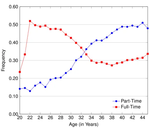
Figure 1.1 shows the share of women working part-time and full-time, respectively. It can be seen that – although part-time and full-time work are similar in terms of total observed person-years (see Table 1.2) – part-time work is relatively rare before age 30 (about 15-20 %), while full-time work is the predominant labor market status (45-50 %) in this age group.9 _{However, part-time work exhibits a steady upward trend, reaching a}

maximum of almost 40 % for ages above 40. Full-time work, on the other hand, decreases and levels off to about 30 % from age 35 on. Despite the possibility for compositional changes driving some of this pattern, it is in line with a fertility-driven reduction in the hours of work over the life-cycle. In fact, Figure1.2confirms that childbearing is highest around the age of 30, when full-time work is decreasing rapidly. The second graph in Figure1.2further shows that the fraction of female households cohabitating with a partner increases in parallel to the birth probability and part-time share, which seems to indicate that the (financial) contribution of the partner to the household (income) is important to explaining life-cycle fertility and employment patterns.

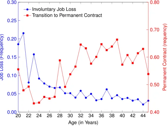
Finally, I emphasize the importance of labor market risks for fertility, female labor supply, and the effectiveness of parental leave policies (see Section 1.1). Figure 1.3

shows that jobs become increasingly secure with age: the probability to lose one’s job exhibits a gradual decline over time, being above 5 % per year for women below the

(32)

20 22 24 26 28 30 32 34 36 38 40 42 44 0.00 0.10 0.20 0.30 0.40 0.50 0.60

Age (in Years)

Frequency

Part-Time Full-Time

Figure 1.1: Distribution of Part-Time and Full-Time Work over Age

Source: Socio-economic Panel, years 1984-2014. This figure shows the shares of women work-ing part-time and full-time relative to all women in the estimation sample.

(33)

1.3. DATA 33 20 22 24 26 28 30 32 34 36 38 40 42 44 0.00 0.10 0.20 0.30 0.40 0.50 0.60 0.70 0.80 0.90 1.00

Age (in Years)

P ar tner in HH (F requency) 0.00 0.02 0.04 0.06 0.08 0.10 0.12 0.14 Child (F requency) Partner in Household Birth of Child

Figure 1.2: Observed Fraction of Women with a Partner and Observed Birth Probabilities by Age

Source: Socio-economic Panel, years 1984-2014. This figure shows the shares of female house-holds in the estimation sample for whom a cohabitating partner is observed, and the age-specific probability of giving birth to a child in the estimation sample.

(34)

age of 30. For higher age groups, the risk to lose one’s job reaches its lowest point around 3 % toward the age of 45. Conversely, the probability to have a permanent job for all previously non-employed or non-permanently employed working women shows an upward age trend, but is consistently high and between 40 and 70 %. Thus, labor market risk declines with age, which might pose a disincentive for having children at younger ages. Importantly, birth probabilities in Figure 1.2 are rising strongest at ages 25-30, which is when labor market risks are reduced most drastically.

20 22 24 26 28 30 32 34 36 38 40 42 44 0.00 0.05 0.10 0.15 0.20 0.25 0.30

Age (in Years)

Job Loss (F requency) 0.40 0.50 0.60 0.70 0.80 Per manent Contr act (requency)

Involuntary Job Loss

Transition to Permanent Contract

Figure 1.3: Risk of Involuntary Job Loss and Transitions to Permanent Contract by Age Source: Socio-economic Panel, years 1984-2014. This figure shows the observed risk of being displaced for employed women and the observed risk of obtaining a permanent work contract for all women who were either non-employed or employed on a fixed-term contract in the previous period.

1.4 Estimation Method

I estimate the model using maximum likelihood estimation, where the likelihood func-tion includes addifunc-tional terms in order to utilize available informafunc-tion on observable labor market shocks. In Section1.4.2, I discuss the identification of labor market frictions in detail.

(35)

1.4. ESTIMATION METHOD 35 1.4.1 Likelihood Function

To define the likelihood function for the dynamic model, first consider that we have four types of data at hand: 1. state variabless ⌘ (sit)i=1,...,N;t=1,...,T with sit being a vector of state variables for observationi, t, 2. choice variablesx ⌘(xit)i=1,...,N;t=1,...,T withxit being the two-dimensional vector of the labor market choicexW

it 2 {N W, P T, F T} and choice of conceptionxC_it 2{C, N C}, 3. labor market frictionsz⌘(zit)i=1,...,N;t=1,...,T such thatzit⌘[zit1, zit2, zit3]denotes job finding, job loss, and transition to a permanent contract, receptively, 4. wageswit, and 5. the stochastic arrival of a partnereit.

Denote the conditional probability density of one observation i, tgiven state sit and model parameters ✓ by f(xit, zit, wit, eit|sit,✓). From the model assumptions, we know thatzitand, eitdo not depend onxit(conditionally onsit) from the timing of labor market, non-labor market shocks and choices, and thatzit andeitare independent conditionally onsit. Similarly, wageswitare independent of(xit, zit, eit)conditionally onsit. Therefore, thei, t-th likelihood contributionL1itcan be written in the following simple form:

e

L1it⌘Le1(✓|xit, zit, wit, eit, sit) = Pr(xit|zit, eit, sit,✓) Pr(zit|sit,✓) Pr(eit|sit,✓)f(wit|sit,✓), (1.12) wherePr(xit|zit, eit, sit,✓)is called the conditional choice probability (CCP) of choicexit, andf denotes the (normal) density function of the wage measurement error. This like-lihood function is, however, not feasible for estimation, since labor market shocksz and wagesware unobserved in many cases.

For wages, this is the case in all periods with no work, i.e. xw_it =N W. Missing wage observations with xw

it 6= N W are assumed to be missing at random. In any case, the likelihood with a missing wage observation is given by

e

L0it⌘Le0(✓|xit, zit, eit, sit) = Pr(xit|zit, eit, sit,✓) Pr(zit|sit,✓) Pr(eit|sit,✓). (1.13) The treatment of missing labor market shocks applies the same logic, but the depen-dence of the CCPs on the realization of the labor market shocks makes things slightly more complicated. Again, we assume that the observability of the variable in question is either fully determined by the observed variables ini, t, or missing at random. The first case arises, for example, when we cannot observe a transition to a permanent contract becausexw

it = N W. Also, as explained in Section1.3the GSOEP does not provide in-formation on job finding, such thatz1 is never observed. In all cases with missing labor market shocks, the likelihood contribution is obtained from integration. Thus, the

(36)

likeli-hood contribution for thei, t-th observation is given by Ljit= 8 > > > > > > > > < > > > > > > > > : P z1 P z3 e Ljit ifzit2 observed, P z1 P z2 e Ljit ifzit3 observed, P z1 e Ljit ifzit2,zit3 observed, P z1 P z2 P z3 e Ljit if nozkitobserved, (1.14) forj₂_{0,1_}andk₂_{1,2,3_}.

1.4.2 Identification of Labor Market Frictions

A vital element of the model of female labor supply and fertility is the effect of work and fertility decisions on future unemployment risk. Classical estimation of the dynamic dis-crete choice model from CCPs alone is not sufficient for estimation in this case. To see this, consider the corresponding fourth case in (1.14). Sincezitis never observed in this case, likelihood estimation solely based on CCPs and wages cannot observationally dis-tinguish a situation with low job availability (low job finding, high job loss) from a situation with high leisure preference. Therefore, information on demand constraints in the labor market is included in the likelihood.

Directly observed labor market shocks are available from the GSOEP for job loss events and a transition to a permanent job contract. Identification of the transition pro-cess from fixed-term to permanent positions is straightforward from all observed such transitions. Given the survey information on a job loss in the recent survey year, it is necessary to distinguish leisure preferences from (unobserved) job finding rates. Fol-lowingHaan and Prowse [2014], leisure preferences can be determined from transitions from work to work when no job loss has been observed (voluntary transition to non-work). Then, job finding probabilities are identified from transitions from non-work into work when a job loss is observed.

1.4.3 Two-Step Estimation

To estimate the parameters of the model, I perform a two-step estimation, where the wage equation (1.4), the observed labor market frictions (job loss and transition to per-manent contract) in (1.5), and the stochastic process for the presence of a partner are estimated in a first step. Estimation of the remaining model parameters, i.e. preference parameters and job finding probabilities, then proceeds by maximizing (1.14) conditional on the pre-estimated parameters. In general, this causes a loss in efficiency compared to joint estimation.

(37)

1.5. RESULTS 37

1.5 Results

In this section, I provide estimation results from a full likelihood based estimation of the dynamic discrete choice model of female labor supply and fertility.10 _{Estimation is}

per-formed using full maximum likelihood estimation as described in Section1.4.1 based on the SOEP data described in Section1.3. Given the utility function, the wage equation and transition equations in Section1.2, assessing the plausibility of the parameter estimates is an important specification check. Moreover, I will discuss the in-sample fit of the two decision margins graphically.

1.5.1 Parameter Estimates

Parameter Estimate (Std.-Err.)

Consumption ⌘ 0.71 (0.33) ! 1.41 (0.07) ↵0 c -1.56 (0.40) ↵1_c,nc 0.46 (0.05) Leisure ↵0 pt 0.46 (0.05) ↵0_{f t} 1.47 (0.07) ↵1 ac,pt -3.19 (0.11) ↵1_{ac,f t} -6.21 (0.13) ↵1 nc,pt 0.25 (0.02) ↵1_{nc,f t} -0.63 (0.03) ↵1_ac,T -5.74 (0.82) Family composition ↵1_ac,t 0.39 (0.02) ↵1 ac,t2 -1.47 (0.12)

Heterogeneity parameters Low edu Mid edu High edu

↵1_nc,edu₌_⇤ -0.02 (0.06) 0.20 (0.05) 0.27 (0.06)

↵1

nc2_,edu₌_⇤ -0.07 (0.01) -0.16 (0.01) -0.20 (0.01)

↵2_edu₌_⇤ 3.45 (0.91) 1.05 (0.85) -0.96 (0.85) Table 1.3: Estimated Parameters of Utility Function

Source: Socio-economic Panel, years 2007-2014. This table shows the observed numbers of all six possible choice combinations for fertility (colums) and labor supply (rows).

(38)

Table1.3 shows the parameter estimates11 _{of the utility function (}_1.1_{). As a whole,}

utility estimates are well in line with economic intuition. First, I estimate a coefficient of relative risk aversion of 0.71, lower than the estimate obtained byAdda et al.[2017]. This is against the backdrop of a lower discount rate ofr = 10%, but without modeling savings. As to the utility parameters for the family composition, the estimation results point to (a) decreasing marginal utility of the total number of children (↵ˆ1_nc,edu₌_⇤ and ↵ˆ1_nc2_,edu₌_⇤),

and (b) an inverted-U shaped age pattern with respect to the utility of having young chil-dren in the household (↵ˆ1

ac,t and↵ˆ1ac,t2). Furthermore, it can be seen that the reference

age for the fertility preferences is roughly 2.5 years later for middle educated than for low educated, and further one year later for the high education group (↵ˆ2_edu₌_⇤).

Parameter estimates on leisure complementarities with family composition are quite plausible. Specifically, there is a positive complementarity between income and family size, as indicated by positive sign of ↵ˆ1_c,nc. Moreover, the inverse age of the youngest childachas a detrimental effect on working for both work categories (↵ˆ1

ac,pt and↵ˆ1ac,f t), which is stronger for full-time work. However, having many children has a negative effect on working full-time (↵ˆ1

nc,f t) but even a positive effect of working part-time (↵ˆ1nc,pt). Est. Std.-Err. 1 edu=2 0.163*** (0.022) 1 edu=3 0.539*** (0.023) 1 exper 0.047*** (0.004) 1 exper2 -0.113*** (0.016) 1 pt -0.078*** (0.011) 0 _{0.206*** (0.025)} N 16,678 AdjustedR2 0.204

Table 1.4: Estimated Parameters of Wage Equation

Source: Socio-economic Panel, years 2007-2014, own calculations. This table shows the estimated parameters of the wage equation (1.4), obtained from a linear regression of the log-arithmic monthly wage in 1,000eon education, experience, and a dummy variable indicating part-time work.

The estimated wage equation in Table1.4shows that accumulating work experience is rewarded in the labor market, with an initial 5 % gain from full-time work (ˆ1

exper) and decreasing returns to experience (ˆ1

exper2). There exists a wage penalty for working

part-time in the amount of 7.8 %.

Turning to the estimates of the labor market frictions in Table1.5, the intuition from ear-lier sections can be confirmed: accumulating human capital through labor supply serves

11_{Parameter estimates shown are for the model with effective maximal parental leave job protection for}

fixed-term contractsPf ix_{of 1 year. Alternative values of}_Pf ix _{= 0}_,₂_,₃_{have been shown to yield inferior} in-sample fit in robustness estimations.

(39)

1.5.

RESUL

TS

39

Find Job Lose Job Get Permanent

Est. Std.-Err. Est. Std.-Err. Est. Std.-Err.

⇤,1 edu=2 0.329*** (0.068) -0.254 (0.172) 0.127 (0.143) ⇤,1 edu=3 0.669*** (0.081) -0.468** (0.184) -0.244 (0.150) ⇤,1 exper -0.051*** (0.014) -0.147*** (0.028) 0.124*** (0.025) ⇤,1 exper2 0.165** (0.073) 0.488*** (0.129) -0.473*** (0.126) ⇤,1 exper3 - - -⇤,1 perm - -1.420*** (0.101) -⇤,0 _{-0.606*** (0.073)} _{-1.045*** (0.187)} _{-0.318** (0.147)} N - 11,624 11,624 Pseudo-R2 _- _0.079 _0.079

Table 1.5: Parameter Estimates of Labor Market Shocks

Source: Socio-economic Panel, years 2007-2014, own calculations. This table shows the estimated parameters of the equations for the labor market frictions in (1.5). The parameters of⇡2

t (job loss shock, column 2) and⇡t3(transition to permanent position, column 3) were obtained from a logistic regression of the binary outcome variables on education and experience, and additionally a dummy variable indicating a permanent work contract in periodt 1for the job loss probability. The parameter estimates for⇡1

(40)

as an insurance in the labor market. This happens via two different channels. First, labor market experience has a negative but decreasing effect on the probability to be displaced (ˆexper2,1 and ˆ_exper2,1 2). Second, there is an indirect channel from transitions to a

perma-nent position: being in a permaperma-nent contract drastically reduces the job loss probability (ˆperm), and gaining experience increases the probability of acquiring such a job contract2,1 (ˆexper3,1 and ˆ_exper3,1 2). These two effects are somewhat offset by a negative but decreasing

effect of labor market experience on the probabiloty to find a new job. Overall, the results show that experience may increase both earnings and job security.

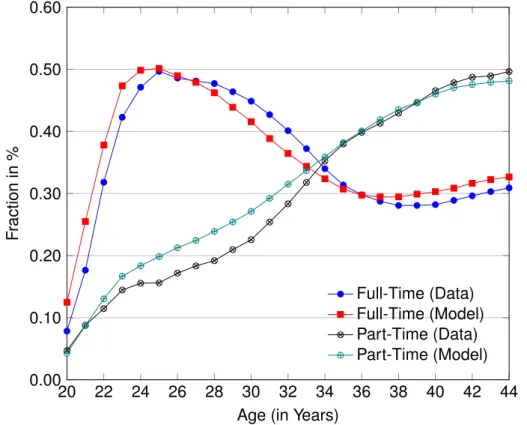
1.5.2 Goodness of Fit

In order to assess the in-sample fit of the estimated structural model, I compare actual to simulated choice frequencies at different ages. To simulate the labor supply and fertility choices I replicated each sample observationM (= 30) times, thus giving me 30 times 23,118 (=693,540) simulated person-years. Then I forward-simulated a complete path of choices and states for each of the 30 times 7,545 (=226,350) synthetic sample members, starting at the age at entry into the sample. When there were missing observations, these observations were set to missing in the simulated sample as well. This simulation tech-nique preserves the sample composition not only in terms of the distribution of education, but also with respect to the distribution of the individual observation window patterns.

The prediction error from forward simulation accumulates with the age of the simu-lated individuals, as misprediced choices feed back into the prediction of the state va-riables. Thus, the fit compares the paths of individual choices observed in the sample. Thus, this is a stricter test for model adequacy than comparing the choice probabilities conditional on the observed values of the state variables. However, the potential for ac-cumulation of large prediction errors over the life-cycle is limited by the fact that only very few individuals exhibit uncensored spells, with a majority of spells being observed less than five time periods.

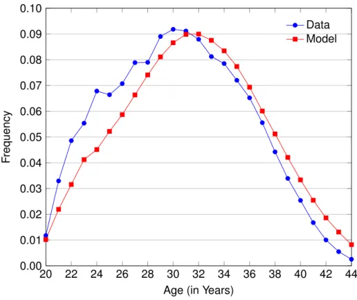
To analyze the goodness of fit, I compared observed and simulated full-time and part-time work proportions for different ages, age-specific average birth probabilities, and the wage distribution. Note that the age patterns shown in the goodness-of-fit statistics are not directly interpretable, as the sample composition (for example in terms of education) changes for different ages due to the generation of the data set described in Appendix

1.B. For the estimation of the model, this is unproblematic as long as the conditional choice probabilities are correctly specified, but the counter-factual policy simulations in Section1.6must account for compositional changes.

Fit of Employment Outcomes Figure1.4shows the fraction of part-time and full-time work over the life-cycle, for the actual and simulated data. Overall, it can be confirmed that the fit looks reasonably well in that the model is able to replicate the marked hump