Reconstruction of parallel MRI Images Using High
Resolution Image Reconstruction Techniques
Raymond H. Chan
∗, I-Liang Chern
†, Chi-Kin Tai
‡and Wen-Yih Isaac Tseng
§ ∗Department of Mathmatics, Chinese University of Hong Kong, Shatin, NT, Hong Kong, ChinaEmail: [email protected]
†Department of Mathematics and Taida Institute of Mathematical Sciences, National Taiwan University, Taipei 106, Taiwan
Email: [email protected]
‡Department of Mathmatics, Chinese University of Hong Kong, Shatin, NT, Hong Kong, China Email: [email protected]
§Center for Optoelectronic Biomedicine, College of Medicine and Department of Medical Imaging, National Taiwan University, Taipei, Taiwan
Email: [email protected]
Abstract— Magnetic resonance imaging (MRI) has been used extensively for clinical purposes to depict anatomy because of its non-invasiveness to human body. It is always desirable to enhance the resolution of MR images in order to confirm the presence of any suspicious behavior inside the body while keeping the imaging time short. In this paper, we change the setting of the k-space sampling which differ from the typical parallel MRI practice. Instead of aliased images, we obtain a number of low resolution coil images. We use two methods, the total variation (TV) inpainting and inpainting in the frequency domain using tight frame, to reconstruct a high resolution image based on these low resolution coil images.
Key words and phrase: MRI, parallel imaging, forward-backward algorithm, total variation.
I. INTRODUCTION
Magnetic resonance imaging (MRI) is a medical imaging technique mainly used to visualize the internal structure and the functions of the body. It provides a greater contrast between the soft tissues of the body than computed tomog-raphy (CT), yet does not involve any ionizing radiation. The magnetic field enables alignment of the nuclear magnetization of NMR-active atoms (mainly hydrogen atoms in water) in the body. This magnetic field, and hence the nuclear magnetiza-tion, is often perturbed by the radio frequency (RF) fields. This generates rotating magnetic fields and in turns induces voltages across the RF coils, which are the MRI signals corresponding to different frequency information of the spins of the hydrogen atoms [10].
Using appropriate samples of the frequency from an array of coils, we can obtain several low resolution images gi with
a blurring operator B. The intensity of the images suffers from the sensitivity effect Ci according to its distance to the
coils. The spatial information of the sensitivity can be used to reconstruct a high resolution image u. This involves solving the following equation,
gi=CiBu+ηi,
where ηi is an additive Gaussian noise. We propose two
methods to reconstruct the desired high resolution image. They are the TV inpainting model [5] and the modified tight frame inpainting in the frequency domain model. The later one is based on the frequency domain inpainting model whose generalization is given in [3]. The details about the formation and the model of the coil images are given in Section 2 and the details of the reconstruction models and the algorithms are given in Section 3.
II. COIL IMAGE FORMATION
A. Introduction to pMRI
A high resolution image of good quality can be obtained from sufficient number of samples in the frequency space (k-space) at the expense of long imaging time. Recently, the development of parallel MRI (pMRI) enables shortening of this sampling time by reducing the number of samples required. With an array of RF coils, some of the spatial coding samples can be skipped by utilizing the spatial sensitivities of individual coils [1]. The MRI signals collected by each coil correspond to the Fourier transform of the image affected by its respective coil sensitivity. The coil sensitivity decays roughly according to the inverse-square-law with respect to the distance to the coil, but the actual sensitivity is difficult to determine because of the complex geometry of the coils.
Most of the pMRI techniques involve skipping the sampling of the k-space data in the phase encoding direction (ky
-direction), causing aliases in the y-direction for each of the coil images. There are well-known techniques concerning the reconstruction of MR images with even contrast and without aliases like SMASH [12], SENSE [11] and GRAPPA [8]. In this work, we propose an alternative way to reconstruct the high resolution image by changing the sampling in the k-space.
B. Model for coil images
We first explain in details how our low resolution images are obtained and their mathematical model. To reduce the imaging time by a factor ofr(which is known as the reduction factor), the usual setting for pMRI is to perform sampling in the k-space with a downsampling factor r in the phase encoding direction, see Fig 1 (center). Since F OVy, the field of view
along the y direction, is inversely proportional to ∆ky, the
space between successiveky-lines,F OVy will be reduced by
the same factorr. This causes aliasing of the coil images in the y-direction. By experimenting in MATLAB [9], for an array consisting of 4 coils, the reconstruction quality is very good for requals to 2.
In our model, we modified the sampling procedures so that only a quarter of the area in the k-space, which is the low frequency part, is sampled, while keeping ∆kx and∆ky
unchanged, see Fig. 1 (right). This prevents the problem of aliasing and instead low resolution images are obtained. It should be noted that r is equal to 2 in this case since only half of the ky lines are sampled. We fix our discussion to this
setting onwards. Fig. 1 illustrates how sampling in thek-space is different for each of the sampling methods.
Fig. 1:k-space samples for full data (left), pMRI (center) and this work (right).
It is obvious that each of our observed coil image gi, i=
1,2, . . . , N,whereNis the number of coils, is a low resolution version of the original true high resolution imageu, together with the effect of its respective coil sensitivity effect [11]. It should be noted that the locations at which the blurring filter is applied are exactly the same since the array of surface coils sample data simultaneously. The model for the coil images is
gi=CiBu+ηi.
Here B is a blurring operator arise from the difference in the sampling procedures for the full k-space data and the low resolution data. In the following we will assume the blurring operator to be the convolution matrix corresponding to the averaging filter l = 1
4[1,2,1] ⊗ 14[1,2,1] with even rows
deleted, together with the reflexive boundary condition. The coil sensitivitiesCi’s are estimated as in [11]. For each
coil, we first estimate the raw coil sensitivity by dividing the coil image by the reference image, which is the sum-of-square (SOS) image of the coil images,gi/
qPN
i=1gi2. A threshold on
the reference image is chosen to identify the noise-free region. A few pixels beyond the noise-free region is identified as the extrapolation zone. We will then perform local polynomial
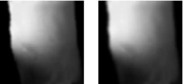
fitting on the raw sensitivity: for each pixel in the noise-free region together with the extrapolation zone, we use a local polynomial with order 2 to fit onto the surrounding noise-free region to estimate the pixel value at the current position. The resulting map is the estimated coil sensitivity. Since the sensitivity functions obtained from the above steps do not vary smoothly, we apply the low-pass filterl as defined above repeatedly to smoothen the result. Fig. 2 shows the estimated coil sensitivityCi before and after treating with the low-pass
filter 20 times.
Fig. 2: Estimated coil sensitvity C1 before (left) and after
treated with B 20 times (right).
III. MODELS FOR THE HIGH RESOLUTION IMAGE RECONSTRUCTION
We will use the proximal forward-backword splitting (FBS) algorithm [2] [7] in the derivation of the tight frame inpainting algorithm and a short review is given in the following. The proof about its convergence can be found at [7].
Consider the minimization problem
min
u {f1(u) +f2(u)}. (1)
withf1(u)a proper, convex and lower semi-continuous
func-tion, andf2(u)a proper, convex, differentiable function with
a1/β continuous gradient. If a minimizer of (1) exists, then with0< δ <2β and arbitrary u0, the iteration
uk+1= arg min v 1 2||u k−δ∇f 2(uk)−v||22+δf1(u) (2) converges to a minimizer of (1).
A. Total variational inpainting approach
We propose the following energy functional to measure the data-fidelity and the smoothness of the reconstructed high-resolution image u, with a parameter λ which controls the significance between the two terms:
Eλ(u) = 1 2 N X i=1 ||CiBu−gi||2+λ||u||T V. (3)
By splitting the functional (3) into two parts f1(u) =λ||u||T V, f2(u) =1 2 N X i=1 ||CiBu−gi||2,
the FBS algorithm (2) reads fk=uk−δ N X i=1 BtCt i(CiBuk−gi), uk+1= arg min v 1 2||u k−fk||2 2+δλ||uk||T V.
Each iteration is a denoising problem and we can use the Chambolle’s method [4] to finduk+1fromfk. The parameter
δ is chosen to be small to guarantee the convergence and the above iteration is run until the change of the reconstructed imageuk is small.
B. Inpainting in the frequency domain using tight frame The inpainting in the image domain algorithm using tight frame is first proposed in [2]. It is easy to modify the algo-rithm to perform instead inpainting in the frequency domain. Interested readers may refer to [3] for a generalization to a simultaneous inpainting in both the image and the frequency domain. The 2D piecewise linear framelets are used in this work. A brief introduction to tight frame and the inpainting algorithm are given below.
The 1D piecewise linear tight framelets are h0=14[1,2,1]
(low part), h1 =
√
2
4 [−1,0,1] and h2 = 14[−1,2,1] (high
parts). The 2D framelets hi,j are formed naturally by using
Kronecker products,hi,j=hi⊗hj fori, j= 0,1,2. Let Hi,j
be the matrices representing the convolution with the filters hi,j. The analysis operatorAis defined as
A= H0,0 H0,1 .. . H2,2 ,
which transform an image u to the transformed domain by left multiplication Au. The multi-level decomposition can be performed by iteratively performing the left-multiplyingAto the low-low parts.
The synthesis operator A∗ is defined correspondingly by the conjugate transpose of A, which recovers an image from the transformed domain. The multi-level synthesis can be performed similarly.
The idea of frequency inpainting is to iteratively extract high-frequency information based on the low resolution im-ages. Since H0,0 is a low pass filter, which is the same as
the filter l in Section 2, we can model the inpainting as given l =H0,0uand aim to find the missing high-frequency
coefficients. This can be done by the algorithm f(r+1)=A∗Tλ((I − PΓ)Af(r)+l).
Here PΓ denotes the projection onto the low-frequency
com-ponent corresponding toH0,0. We denote the sizes of the high
resolution image be M1,M2, andTλ is the soft-thresholding
function withλequal to
λ(r)i,j =σˆ(r)i,jp2 log(M1M2). (4)
The noise level σˆ(r)i,j is estimated by the median of the
coefficients in the subband divided by the constant 0.6745 [6]. It has been proved in [3] that the algorithm converges to the limitf which solves the following minimization,
min c 1 2||PΓ(c−d)|| 2 2+ 1 2||(I− AA ∗)c||2 2+||diag(λ)c||1, wherec=Af.
For our problem, apart from the blurring phenomenon, there is also the sensitivity effect depending on the coil location which affects each of the low resolution coil image. To fit into this model, we modify the energy functional to be
min c { 4 X i=1 1 2||CiBA ∗c−g i||22+ 1 2||(I−AA ∗)c||2 2+||diag(λ)c||1}.
The proximal forward-backward splitting [7] [2] is applied to solve this minimization. We split the above functional into two parts, f1(c) =||diag(λ)c||1, f2(c) = 4 X i=1 1 2||CiBA ∗c−g i||22+ 1 2||(I− AA ∗)c||2 2.
The corresponding proximal forward-backward splitting algo-rithm reads, ck+1 2 =ck−µ[ 4 X i=1 (ABTC i)(CiBA∗ck−gi) + (I− AA∗)ck], ck+1=T λµ(ck+ 1 2).
We use the same way as in (4) to estimate the noise level σ(r)i,j, and henceλ(r)i,j. The algorithm is run until the difference between successive reconstructed images is small. Note that the limit of the algorithm does not depends on µ, yet µ has to be sufficiently small to guarantee the convergence.
IV. RESULTS
A. Simulation
To test the performance of the two reconstruction methods in Section 3, the SOS reconstructed brain MR image from [9] is used as the original image. We use an array of 4 coils. The sensitivity profiles Ci’s are simulated by the followings
according roughly to the inverse-square law:
C1(x, y) = 8000/(25000 + (x+ 40)2+ (y+ 10)2),
C2(x, y) = 8000/(25000 + (x+ 45)2+ (y−290)2),
C3(x, y) = 8000/(25000 + (x−300)2+ (y+ 15)2),
C4(x, y) = 8000/(25000 + (x−280)2+ (y−315)2).
The true image is degraded by respective sensitivity, and their low frequency parts in the k-space are sub-sampled to obtain the low resolution coil images, which are further degraded by additive white Gaussian noises with standard deviationσ= 5. The central part of the image is chosen to be the region of interest (ROI). Fig. 3 shows the noisy low resolution images
(a)
(b)
Fig. 3: (a) Simulated noisy coil images and (b) the original image under ROI in this experiment.
and the central part of the original image which is taken as the true image to compare the reconstruction methods.
To compare the performance of the two reconstruction algorithms, we use the simulated sensitivity functions in the coarse grid in the reconstruction process. We implement the two algorithms in Section 3 in MATLAB to reconstruct the high resolution images. The parameterλis chosen to be 0.001 in the TV inpainting approach and the level of decomposition is chosen to be 2 in the frequency inpainting approach by trial and error for good reconstruction quality. The SOS re-construction which is enlarged by bicubic interpolation is also compared for reference. Fig. 4 shows the reconstructed results. The frequency inpainting reconstruction performs better both numerically and visually. The details can be seen more clearly in the image.
B. Clinical data
We use images that are obtained in the real MRI knee examination. A phase array consisting of 4 coils is used, giving 4 low resolution coil images affected by their respective coil sensitivity. Fig. 5 shows the 4 coil images gi, i = 1,2,3,4.
The procedures in Section 2 are performed to obtain the sensitivity profiles. Algorithms in Section 3 are implemented to obtain the reconstructed images. Again, we give the SOS image enlarged by bicubic interpolation for comparison. The parameter λ is set to be 2 for the TV inpainting approach
(a)
(b)
(c)
Fig. 4: Reconstructed images by (a) TV inpainting (PSNR = 26.78dB), (b) frequency domain inpainting (PSNR = 26.98dB) amd (c) SOS (PSNR = 25.08dB).
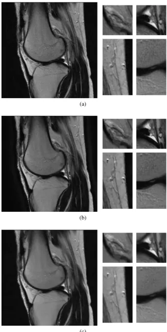
and the level of decomposition is set to be 3 for the frequecy domain inpainting approach. Fig. 6 shows the reconstructed results together with the enlarged SOS image. The zooms into some of the details are also given. We can see from the figure that both reconstructed results show less blocky or jaggy features, and with clearer features where a suitable level of denoising is incorporated in the algorithms. The two proposed reconstruction gives results merely differ from contrast but no obvious difference.
V. CONCLUSION
We discussed an alternative image reconstruction method based on a different sampling of the k-space which differs from the traditional pMRI techniques. Two algorithms are given with good reconstruction qualities. They have compa-rable performances but the reconstruction from inpainting in the frequency domain approach seems to recover the details in an image better. It is clear that improvements can be made to this work say by giving a better blurring operator, or finding a better reconstructed image based on other models. Overall this work provides a direct way for reconstructing MR images
Fig. 5: 4 coil images gi’s with different coil sensitivities.
which does not involve aliasing nor estimating data in the k-space. Only rough estimates of the sensitivities are required as they only have slight effect on the contrast to the final images. Although the comparison with other pMRI techniques is unclear at the moment, it is hoped that this idea can lead to alternative models with better reconstruction quality or shorter imaging time.
ACKNOWLEDGMENT
The authors thank Maoyuan Su from the National Taiwan University Hospital for providing the practical MR knee images; and Haixia Liang and Yiqiu Dong for their helpful discussions.
REFERENCES
[1] M. Blaimer, F. Breuer, M. Mueller, R. M. Heidemann, Mark A. Griswold, and Peter M. Jakob, “SMASH, SENSE, PILS, GRAPPA. How to choose the optimal method,”Top Magn Reson Imaging, vol. 15, pp. 223-236, 2004.
[2] J.F. Cai, R. Chan, and Z. W. Shen, “A Framelet-Based Image Inpainting Algorithm,”Appl. Comput. Harmon. Anal., vol. 24, pp. 131-149, 2008. [3] J.F. Cai, R. Chan, L. X. Shen, and Z. W. Shen, “Simultaneously Inpainting
in Image and Transformed Domains,”Numer. Math., vol. 112, pp. 509-533, 2009.
[4] A. Chambolle, “An Algorithm for Total Variation Minimization and Applications,”J. Math. Imaging and Vision, vol. 20 (1-2): pp. 89-97, 2004.
[5] T. F. Chan, M. K. Ng, A. C. Yau, and A. M. Yip, “Superresolution image reconstruction using fast inpainting algorithms,”Applied and Computa-tional Harmonic Anal., vol. 23, Issue 1, Special Issue on Mathematical Imaging, pp. 3-24, 2007.
[6] S. G. Chang, B. Yu, and M. Vetterli, “Adaptive wavelet thresholding for image denoising and compression,”IEEE Trans. Img. Proc., vol. 9, no. 9, pp. 1532-1546, 2000.
[7] P. Combettes and V. Wajs, “Signal recovery by proximal forward-backward splitting,”SIAM Journal on Multiscale Modeling & Simulation, vol. 4, pp. 1168-1200, 2005.
[8] Mark A. Griswold, Peter M. Jakob , Robin M. Heidemann, Mathias Nittka, Vladimir Jellus, Jianmin Wang, Berthold Kiefer, and Axel Haase, “Generalized autocalibrating partially parallel acquisitions (GRAPPA),”
Magn. Reson. Med., vol. 47, pp. 1202-1210, 2002.
(a)
(b)
(c)
Fig. 6: Comparison of the reconstructed images with zooms. (a) SOS with enlargement by bicubic interpolation. (b) TV inpainting approach. (c) inpainting in the frequency domain using tight frame.
[9] J. X. Ji, J. B. Son, and S. D. Rane, “PULSAR: A Matlab toolbox for parallel magnetic resonance imaging using array coils and multiple channel receivers,”Concepts Magn Reson B., vol. 31B, Issue 1, pp. 24-36, 2007.
[10] R. A. Novelline, and L. F. Squire,Squire’s Fundamentals of Radiology, 5th ed. Cambridge: Harvard University Press, 1997.
[11] K. P. Pruessmann, M. Weiger, M. B. Scheidegger, and P. Boesiger, “SENSE: sensitivity encoding for fast MRI,”Magn. Reson. Med., vol. 42, no. 5, pp. 952-962, 1999.
[12] D. K. Sodickson, and W. J. Manning, “Simultaneous acquisition of spatial harmonics (SMASH): Fast imaging with radiofrequency coil arrays,”Magn. Reson. Med., vol. 38, pp.591-603, 1997.