An High Equipped Image Reconstruction Framework Based on Morphologic Regularization approach Using Bregman Iteration SR algorithm

Available online: https://edupediapublications.org/journals/index.php/IJR/ P a g e | 1586

An High Equipped Image Reconstruction Framework Based on

Morphologic Regularization approach Using Bregman Iteration SR

algorithm

Prashant B. Raule & Ravindra P. Shelkikar

(M.E. Scholar)1 _{(Associate Professor)}2

Electronics and Telecommunication Engineering Department1,2

1,2_{TPCT’s College of Engineering, District-Osmanabad, (M.S.), India.}

1_{[email protected]} 2_{[email protected]}

A

bstract

Feature extractions are the novel techniques in image

processing to store its unique characteristics.

Morphological operators are the best for any image

processing applications because it helps to preserve some

characteristics from image. Although morphological

operators is successful in solving the feature extraction but

it too has some drawbacks. In this paper we model a non

linear regularization method based on multi scale

morphology for edge preserving super resolution (SR)

image reconstruction. We formulate SR reconstruction

problem from low resolution (LR) image as a deblurring

and denoising and then solve the inverse problem using

Bregman iterations. The proposed Method can be reduce

inherent noise generated during low-resolution image

formation as well as during SR image estimation efficiently.

Using MATLAB simulation results we showed the

effectiveness of the proposed method and reconstruction

method for SR image.

I.

I

NRODUCTION

The basic goal is to develop an algorithm to enhance

the spatial resolution of images captured by an image

sensor with a fixed resolution. This process is called the

super resolution (SR) method and it has remained an active

research topic for the last two decades.

Super-resolution (SR) technique reconstructs a higher-Super-resolution

image or sequence from the observed LR images. As SR

has been developed for more than three decades, both

multi-frame and single-frame SR have significant

applications in our daily life.SR algorithms may vary

depending on whether only a single low-resolution (LR)

image is available (single frame SR) or multiple LR images

are available (multi frame SR).

SR image reconstruction algorithms work either:

1) In the frequency domain or

2) In the spatial domain.

This paper focus only on spatial domain approach

for multi frame SR image reconstruction. This paper is

based on the regularization framework, where the HR

image is estimated based on some prior knowledge about

the image (e.g., degree of smoothness) in the form of

regularization.

Bayesian maximum a posteriori (MAP) estimation

based methods use prior information in the form of a prior

probability density on the HR image and provides a

Available online: https://edupediapublications.org/journals/index.php/IJR/ P a g e | 1587 formulation is proposed that judiciously combine motion

estimation, segmentation, and SR together. The probability

based MAP approach is equivalent to the concept of

regularization. he first successful edge preserving

regularization method for denoising and deblurring is the

total variance (TV) (L1 norm) method. Another interesting

algorithm, proposed by Farsiu et al., employs bilateral total

variation (BTV) regularization.

SR is a technique which reconstructs a higher-resolution

image or sequence from the observed LR images.

Technically, SR can be

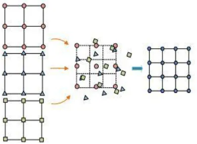
Fig. 1. The concept of multi-frame super-resolution. The grids on the left side represent the LR images of the same

scene with sub-pixel alignment, thus the HR image (the

grid on the right side) can be acquired by fusing the

complementary information with SR methods.

A new regularization method based on multi scale morphologic filters is proposed, which are nonlinear in

nature. Morphological operators and filters are well-known

tools that can extract structures from images. Since

proposed morphologic regularization term uses non

differentiable max and min operators, developed an

algorithm based on Bregman iterations and the forward

backward operator splitting using sub gradients. The results

produced by the proposed regularization are less affected

by aforementioned noise evolved during the iterative

process.

II.

P

ROBLEM

F

ORMULATION

The observed images of a scene are usually degraded

by blurring due to atmospheric turbulence and

inappropriate camera settings. The LR images are further

degraded because of down sampling by a factor determined

by the intrinsic camera parameters. The relationship

between the LR images and the HR image can be

formulated as

𝑌𝑘= 𝐷𝐹𝑘𝐻𝑘𝑋 + 𝑒𝑘, ∀𝑘 = 1, 2, … , 𝐾 (1)

where Yk , X, and ek represent lexicographically ordered

column vectors of the kth LR image of size M, HR image

of size N and additive noise, respectively. FK is a geometric

warp matrix and HK is the blurring matrix of size N×N

incorporating camera lens/CCD blurring as well as

atmospheric blurring. D is the down sampling matrix of

size M × N and k is the index of the LR images. Assuming

that the LR images are taken under the same environmental

condition and using same sensor, HK becomes the same for

all k and may be denoted simply by H. the LR images are

related to the HR image as

𝑌𝑘 = 𝐷𝐹𝑘𝐻𝑋 + 𝑒𝑘, ∀𝑘 = 1, 2, … , 𝐾 (2)

Since under assumption, D and H are the same for all LR

images, avoid down sampling and then up sampling at each

iteration of iterative reconstruction algorithm by merging

the up sampled and shifted-back LR images Yk together.

After applying up sampling and reverse shifting, Yk will be

aligned with HR image X. Suppose Yk denotes the up

sampled and reverse-shifted kth LR image obtained through

Available online: https://edupediapublications.org/journals/index.php/IJR/ P a g e | 1588 where DT is the up sampling operator matrix of size N × M

and is an N × N matrix that shifts back (reverse effect of FK

) the image. The equation from (2), (3), (4) as,

𝑌 = 𝑅𝐻𝑋 + 𝑒 (3)

𝑋̂ = 𝑎𝑟𝑔 min

𝑋 [‖𝑅𝐻𝑋 − 𝑌‖2

2

] (4)

Regularization has used in conjunction with iterative

methods for the restoration of noisy degraded images in

order to solve an ill-posed problem and prevent over-fitting.

Then the SR image reconstruction can simply be

formulated as

𝑋̂ = 𝑎𝑟𝑔 min

𝑋 [Υ(𝑋) ∶ ‖𝑅𝐻𝑋 − 𝑌‖2

2

< 𝜂] (5)

Where η is a scalar constant depending on the noise

variance in the LR images

III.

P

ROPOSED

W

ORK

A.

M

R

Let B be a disk of unit size with origin at its center and

SB be a disk structuring element (SE) of size s. Then the

morphological dilation DS (X) of an image X of size M X

N at scale S is defined as

𝐷𝑠(𝑋) =

(

𝑚𝑎𝑥𝑟∈(𝑠𝐵)₍₁₎{𝑥𝑟}

𝑚𝑎𝑥𝑟∈(𝑠𝐵)₍₂₎{𝑥𝑟}

⋱

𝑚𝑎𝑥𝑟∈(𝑠𝐵)_(𝑚𝑛){𝑥𝑟}₎

(6)

Where (SB)(I ) is a set of pixels covered under SE SB

translated to the I -th pixel XI . Similarly, the

morphological erosion ES (X) at scale S is defined as

𝐸𝑠(𝑋) =

( min

𝑟∈(𝑠𝐵)(1){𝑥𝑟}

min

𝑟∈(𝑠𝐵)(2){𝑥𝑟}

. . . min 𝑟∈(𝑠𝐵)(𝑚𝑛){𝑥𝑟}) (7)

Morphological opening OS (X) and closing CS (X) by SE

SB are defined as follows:

𝑂𝑠(𝑋) = 𝐷𝑠(𝐸𝑠(𝑋)) (8)

𝐶𝑠(𝑋) = 𝐸𝑠(𝐷𝑠(𝑋)) (9)

In multi scale morphological image analysis, the difference

between the sth _{scale closing and opening extracts noise}

particles and image artifacts in scale S and may be used for

denoising purposes.

B.

S

M

B

I

Bregman iteration is used in the field of computer

vision for finding the optimal value of energy functions in

the form of a constrained convex functional. In constrained and unconstrained problems, the “fixed point continuation”

(FPC) method is used to solve the unconstrained problem

by performing gradient descent steps iteratively. The

linearized Bregman algorithm is derived by combining the

FPC and Bregman iteration to solve the constrained

problem in a more efficient way. An algorithm is developed

on Bregman iteration and the proposed morphologic

regularization for the SR image reconstruction problem.

C.

B

I

The proposed penalized splitting approach and corresponds

to an algorithm whose structure is characterized by

Available online: https://edupediapublications.org/journals/index.php/IJR/ P a g e | 1589 the convergence to the global minimum, and an inner loop,

which iteratively, using the two-step approach, minimizes the penalization function for the given value of λ. The

general scheme of the bound constrained algorithm is the

following.

Initialize Y(0)_{= n = 0, 𝑌, X}(0)_{= FillUnknown(Y);}

While(‖𝑅𝐻𝑋(𝑛)_{− Y‖} 2 2

> 𝜂)

{

𝑈(𝑛+1)_{= X}(𝑛)_{− 𝛾𝐻}𝑇_𝑅𝑇_(RHX(n)_{− Y}(𝑛)₎

𝑋(𝑛+1)_{= 𝑈}(𝑛+1)_{− 𝜇}′_|𝛿Υ(X) 𝛿(X)|_X(𝑛)

𝑌(𝑛+1)_{= 𝑌}(𝑛)_{+ (𝑌 − 𝑅𝐻𝑋}(𝑛+1)₎

𝑛 = 𝑛 + 1

(10)

Here we derive the sub gradients of the dilated and eroded

image with respect to its pixel values. Let us denote the sub

gradient of a dilated image Ds(X)

𝛿𝐷𝑠,𝑗

𝛿𝑥𝑖

=

{

1, if 𝑥𝑖= max_{𝑟𝜖(𝑠𝐵)} (𝑗)

{𝑥𝑟} 𝑎𝑛𝑑

∀𝑡 ∈ (𝑠𝐵)(𝑗), 𝑡 ≠ 𝑖, 𝑥𝑡< 𝑥𝑖

0, if 𝑥𝑖< max 𝑟𝜖(𝑠𝐵)_(𝑗){𝑥𝑟}

𝜖[0,1], elsewhere

(11)

Similarly, the sub gradient of an eroded image Es(X) can be

written as follows. We choose the sub gradient equal to 1

out of the range [0, 1]. Then the sub gradients become

𝛿𝐷𝑠,𝑗

𝛿𝑥𝑖

= {

1, if 𝑥𝑖= max 𝑟𝜖(𝑠𝐵)(𝑗)

{𝑥𝑟}

0, if 𝑥𝑖< max 𝑟𝜖(𝑠𝐵)(𝑗) {𝑥𝑟} (12) 𝛿𝐸𝑠,𝑗 𝛿𝑥𝑖 = {

1, if 𝑥𝑖= max 𝑟𝜖(𝑠𝐵)_(𝑗){𝑥𝑟}

0, if 𝑥𝑖< max 𝑟𝜖(𝑠𝐵)_(𝑗){𝑥𝑟}

(13)

Since an analogous chain rule holds for the sub gradients,

we can write down the sub gradients of the regularization

function

𝛿Υ(X)

𝛿(X) ∶=

𝛿

𝛿X∑ 𝛼

𝑠₁𝑡_[𝐶

𝑠(𝑋) − 𝑂𝑠(𝑋)] 𝐾

𝑠=1

= ∑ 𝛼𝑠_[𝛿𝐶𝑠(X)

𝛿X −

𝛿𝑂𝑠(X)

𝛿X ] 1

𝐾

𝑠=1

= ∑ 𝛼𝑠_[𝛿

𝛿X𝐸𝑠(𝐷𝑠(𝑋)) − 𝛿

𝛿X𝐷𝑠(𝐸𝑠(𝑋))] 1

𝐾 𝑠=1 = ∑ 𝛼𝑠_[ 𝛿 𝛿𝐷𝑠(𝑋) 𝐸𝑠(𝐷𝑠(𝑋)) 𝛿

𝛿X𝐷𝑠(𝑋)]

𝐾 𝑠=1 − [ 𝛿 𝛿𝐸𝑠(𝑋) 𝐷𝑠(𝐸𝑠(𝑋)) 𝛿

𝛿X𝐸𝑠(𝑋)] 1 (14)

The respective erosion and dilution functions are illustrated

as follows

𝑞_𝑖𝐸𝑠,𝑗_{: =}𝛿𝐸𝑠,𝑗

𝛿𝑑𝑠,𝑖

= {

1, if 𝑑𝑠,𝑖= max_{𝑟𝜖(𝑠𝐵)} (𝑗)

{𝑑_𝑠,𝑖}

0, if 𝑑𝑠,𝑖< max 𝑟𝜖(𝑠𝐵)(𝑗) {𝑑𝑠,𝑖} (15) 𝑞_𝑖𝐷𝑠𝑠,𝑗: =𝛿𝐷𝑠,𝑗 𝛿𝑒𝑠,𝑖 = {

1, if 𝑒𝑠,𝑖= max 𝑟𝜖(𝑠𝐵)_(𝑗){𝑒𝑠,𝑖}

0, if 𝑒𝑠,𝑖< max 𝑟𝜖(𝑠𝐵)_(𝑗){𝑒𝑠,𝑖}

(16)

IV.

S

IMULATION

R

ESULTS

Available online: https://edupediapublications.org/journals/index.php/IJR/ P a g e | 1590 Figure 2 Comparison of reconstruction result of the chart

image for misestimated motion model and erroneous

Gaussian blur parameter. SR image reconstruction using (a)

Grd +BTV

Figure 3 Comparison of reconstruction result of the chart image for misestimated motion model and erroneous

Gaussian blur parameter. SR image reconstruction using (b)

Breg+BTV

Figure 4 Comparison of reconstruction result of the chart image for misestimated motion model and erroneous

Gaussian blur parameter. SR image reconstruction using (c)

Breg +Morph (proposed method)

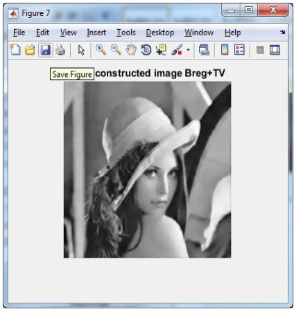
Available online: https://edupediapublications.org/journals/index.php/IJR/ P a g e | 1591 Gaussian blur parameter. SR image reconstruction using (c)

Breg +TV .

B.

R

ESULTS

F

OR SR2

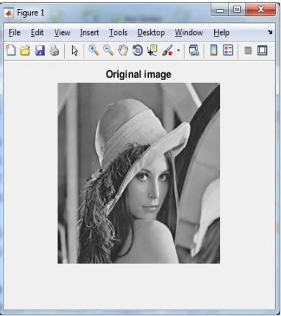
Figure 6 Results of the various SR image reconstruction methods with a small amount of noise (σ=2). (a) Original HR image of a chart.

Figure 7 Results of the various SR image reconstruction methods with a small amount of noise (σ=2). (b) One of the

generated LR images.

Figure 8 Results of the various SR image reconstruction methods with a small amount of noise (σ=2). (c) Up

sampled and merged 10 LR images.

Available online: https://edupediapublications.org/journals/index.php/IJR/ P a g e | 1592 reconstructed image using the gradient descent method with

TV,BTV, and LABTV regularization, respectively.

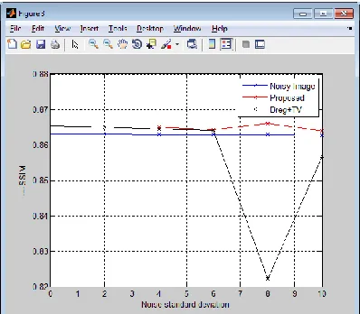
Figure 10 Analysis of the performance of SR image reconstruction algorithms applied on different gray images

and then average quantitative measures are plotted. (a)

PSNR and SSIM of SR algorithms for noisy LR images

with additive Gaussian noise.

Figure 11 Analysis of the performance of SR image reconstruction algorithms applied on different gray images

and then average quantitative measures are plotted. (b)

PSNR and SSIM for different amount of misrediction in the

blurring parameter.

Table 1: Time required to execute the existing system(Breg+TV) and proposed work(Breg+Morph)

We studied theoretically that proposed work require less

time for execution compared to state of art existing

techniques.

Figure 12 log of residue versus no of iterations plot

Here, we plotted log of residue versus no of iterations plot,

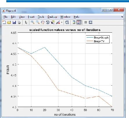
Available online: https://edupediapublications.org/journals/index.php/IJR/ P a g e | 1593 Figure 13 scaled function values versus no. of iterations.

These two plots, i.e., Fig.11 and 12, together show the reconstruction qualities of different methods with number of iterations.

Table 2: Comparative analysis of Existing (Breg+TV) and Proposed (Breg+Morph) Method

Different

Images

Breg+ TV Proposed Method

PSNR SSIM PSNR SSIM

30.4438 0.9940 35.6078 0.9948

29.0320 0.9343 33.0751 0.9315

27.2429 0.9735 32.1092 0.9730

26.3673 0.9758 31.1846 0.9739

28.2611 0.9921 34.1718 0.9934

26.7441 0.8985 31.8901 0.8966

27.6456 0.9943 33.0662 0.9938

28.1086 0.9769 33.1717 0.9769

23.6189 0.9780 28.1661 0.9786

26.2741 0.9915 31.1790 0.9916



Applications

1.Regular video information enhancement

2. Surveillance

3. Medical diagnosis

4. Earth-observation remote sensing

5. Astronomical observation

6. Biometric information identification

V.

C

ONCLUSION

This paper presented an edge-preserving SR image

reconstruction problem as a deblurring problem with a new

robust morphologic regularization method. Then put

forward two major contributions. First, proposed a

morphologic regularization function based on multi scale

opening and closing, which could remove noise efficiently

while preserving edge information. Next, employed

Bregman iteration method to solve the inverse problem for

SR reconstruction with the proposed morphologic

regularization. Compare to previous algorithms proposed

algorithm gives better results of quality parameters.Matlab

simulations also shows that the proposed work is more

efficient compared to all other existing techniques. For

quality assessment we are going to use two parameters as

PSNR and SSIM.It is known that multi scale morphological

filtering can reduce noise efficiently, so a successfully

regularization method is used based on multi scale

morphology. The experimental results show that it works

quite well, in fact better than existing methods.

Nonlinearity of the regularization function is handled in a

linear fashion during optimization by means of the sub

Available online: https://edupediapublications.org/journals/index.php/IJR/ P a g e | 1594 regularization method proposed here was tested only on SR

reconstruction problem; this method is extended by

computing Blocking effect, Homogeneity and ISNR.

R

EFERENCES

[1] S. Lertrattanapanich and N. K. Bose, “High resolution

image formation from low resolution frames using Delaunay triangulation,” IEEE Trans. Image Process., vol.

11, no. 12, pp. 1427–1441, Dec. 2002.

[2] A. J. Patti and Y. Altunbasak, “Artifact reduction for set

theoretic super resolution image reconstruction with edge

adaptive constraints and higher-order interpolants,” IEEE

Trans. Image Process., vol. 10, no. 1, pp. 179–186, Jan.

2001.

[3] M. Elad and A. Feuer, “Restoration of a single super

resolution image from several blurred, noisy and under sampled measured images,” IEEE Trans. Image Process.,

vol. 6, no. 12, pp. 1646–1658, Dec. 1997.

[4] H. Shen, L. Zhang, B. Huang, and P. Li, “A MAP

approach for joint motion estimation segmentation and super resolution,” IEEE Trans. Image Process., vol. 16, no.

2, pp. 479–490, Feb. 2007.

[5] W. T. Freeman and T. R. Jones, “Example-based super resolution,” IEEE Comput. Graphics Appl., vol. 22, no. 2,

pp. 56–65, Mar. 2002.

[6] J. Yang, J. Wright, T. S. Huang, and Y. Ma, “Image

super-resolution via sparse representation,” IEEE Trans.

Image Process., vol. 19, no. 11, pp.2861–2873, Nov. 2010.

[7] K. I. Kim and Y. Kwon, “Single-image super resolution using sparse regression and natural image prior,” IEEE

Trans. Pattern Anal. Mach. Intell., vol. 32, no. 6, pp. 1127–

1133, Jun. 2010.

[8] W. Dong, L. Zhang, G. Shi, and X. Wu, “Image

deblurring and super resolution by adaptive sparse domain selection and adaptive regularization,” IEEE Trans. Image

Process., vol. 20, no. 7, pp. 533–549, Jul. 2011.

[9] M. Protter, M. Elad, H. Takeda, and P. Milanfar, “Generalizing the nonlocal-means to super-resolution reconstruction,” IEEE Trans. Image Process., vol. 18, no. 1,