Dynamic Risk Exposure in Hedge Funds
∗
Monica Billio
†, Mila Getmansky
‡and
Loriana Pelizzon
§This Draft: January 11, 2008
Abstract
We measure dynamic risk exposure of hedge funds to various risk factors during different market volatility conditions using the regime-switching beta model. We find that in the high-volatility regime (when the market is rolling-down) most of the strategies are negatively and significantly exposed to the Large-Small and Credit Spread risk factors. This suggests that liquidity risk and credit risk are potentially common factors for different hedge fund strategies in the down-state of the market, when volatility is high and returns are very low. We further explore the possibility that all hedge fund strategies exhibit idiosyncratic risk in a high volatility regime and find that the joint probability jumps from approximately 0% to almost 100% only during the Long-Term Capital Management (LTCM) crisis. Out-of-sample forecasting tests confirm the economic importance of accounting for the presence of market volatility regimes in determining hedge funds risk exposure.
Keywords: Hedge Funds; Risk Management; Regime-Switching Models; JEL Classification: G12, G29, C51
∗We thank Vikas Agarwal, Lieven Baele, Ben Branch, Stephen Brown, Laura Frieder, Bruno Gerard,
David Hsieh, William Fung, Will Goetzmann, Robin Greenwood, Ravi Jagannathan, Nikunj Kapadia, Hos-sein Kazemi, Camelia Kuhnen, Martin Lettau, Bing Liang, Laura Lindsay, Andrew Lo, Narayan Naik, Geert Rouwenhorst, Stephen Schaefer, Tom Schneeweis, Matthew Spiegel, Heather Tookes, Marno Verbeek, Pietro Veronesi, Rebecca Zarutskie and seminar participants at the NYU Stern School of Business, Cornell, Rut-gers Business School, University of Waterloo, Hebrew University, Brandeis University, State University of New York-Albany, University of Massachusetts-Amherst, University of Connecticut, Tilburg University, Sor-bonne University-CES Paris 1, Goethe University, ENS CACHAN, European Finance Association Conference (EFA), European Summer Symposium in Financial Markets (ESSFM), Second Italian Conference in Econo-metrics and Empirical Economics, International Workshop on Computational and Financial EconoEcono-metrics,
and European Conference of the Econometric Community (EC2) for valuable comments and suggestions.
†University of Venice and SSAV, Department of Economics, Fondamenta San Giobbe 873, 30100 Venice,
(39) 041 234–9170 (voice), (39) 041 234–9176 (fax),[email protected](e-mail).
‡Isenberg School of Management, University of Massachusetts, 121 Presidents Drive, Room 308C,
Amherst, MA 01003, (413) 577–3308 (voice), (413) 545–3858 (fax),[email protected](e-mail).
§University of Venice and SSAV, Department of Economics, Fondamenta San Giobbe 873, 30100 Venice,
1
Introduction
The last decade has seen an increase in the number of hedge funds and the availability of hedge fund data both on individual hedge funds and on hedge fund indexes. Unlike mutual funds, hedge funds engage in dynamic strategies, use leverage, take concentrated bets, bet on volatility and have non-linear payoffs. The tremendous increase in the number of hedge funds and the availability of hedge fund data has attracted a lot of attention in the academic literature, which has been concentrated on analyzing hedge fund styles (Fung and Hsieh (2001) and Mitchell and Pulvino (2001)), performance and risk exposure (Fung and Hsieh (1997), Brealey and Kaplanis (2001), Edwards and Caglayan (2001), Agarwal and Naik (2004), Bali, Gokcan and Liang (2007), Gupta and Liang (2005), and Schneeweis, Karavas, and Georgiev (2002)), liquidity, systemic risk and contagion issues (Getmansky, Lo, and Makarov (2004), Chan, Getmansky, Haas, and Lo (2005) and Boyson, Stahel and Stulz (2006)).
The aim of this paper is to analyze time-varying and state-dependent risk exposures for various hedge fund strategies and obtain reliable estimates for predicted exposures of hedge fund returns. The innovative aspect of this paper is that we study hedge fund risk exposure conditional on different levels of mean and volatility of the market risk factor, characterized by the S&P 500.
Understanding and modeling hedge fund risk exposures is fundamental for both hedge fund investors and regulators. For example, the recent subprime mortgage crisis of August 2007 exposed new types of risk for hedge funds, and currently there is a discussion of a potential role of regulators to diminish the effects of this crisis. This crisis also emphasized the importance of credit and liquidity for hedge fund returns. For investors, a knowledge of hedge fund exposures is essential in order to analyze risk-adjusted hedge fund performance and to perform optimal asset allocation. Regulators are concerned about risks that are common across different hedge fund strategies. These risks can be responsible for financial trouble in the hedge fund industry and can act as catalysts for a spillover to other financial sectors, i.e., systemic risk. Moreover, regulators are worried if this joint risk across hedge fund strategies is associated with a particular state or regime of the equity market. In addition, regulators are concerned about an event where all different hedge fund strategies move to a high volatility state due to liquidity or non-market related shocks. This can lead to the downfall of all hedge fund strategies at the same time and potential spillovers to financial markets.
applied in stress-testing analysis.
Hedge funds may exhibit non-normal payoffs for various reasons such as their use of options, or more generally dynamic trading strategies. Unlike most mutual funds (Koski and Pontiff (1999) and Almazan et al. (2004)), hedge funds frequently trade in derivatives. Further, hedge funds are known for the “opportunistic” nature of their trading strategies and a significant part of their returns arise from taking state-contingent and volatility bets. There is currently a limited understanding of the real non-linear exposure to risk factors of the different hedge funds strategies. In the hedge fund literature, the analysis of risk exposure is based on three main approaches. The first approach is based on the classical linear factor model applied to mutual funds. The second, introduced by Fung and Hsieh (1997), is based on a predetermined structure of the risk factors (quintile analysis or extreme event analysis). The third approach is based on option-like payoffs, also called Asset-Based Style Factors (ABS-Factors), introduced by Fung and Hsieh (2001) and Agarwal and Naik (2004). We add to the literature by proposing a new way of capturing dynamic risk exposure in hedge funds based on volatility changes of the market risk factor.
In this paper, consistent with the asset pricing perspective proposed by Bekaert and Harvey (1995), we suggest analyzing the exposure of hedge fund indexes with a factor model based on regime-switching volatility, where non-linearity in the exposure is captured by factor loadings that are state-dependent. The regime-switching approach is able to identify when the market risk factor is characterized by normal, down-market or up-market conditions, and the state dependent factor loadings are able to capture the exposure of hedge funds to risk factors in these different volatility states.1 To our knowledge this is the first attempt
to analyze hedge fund exposure considering that the market risk factor is characterized by stochastic volatility, i.e., calculating hedge fund exposure to the market factor by explicitly accounting for the change in volatility of the market factor. This feature is relevant because hedge funds bet on volatility, and factor loadings are affected by the volatility of the risk factors.
The importance of using regime-switching models is well established in the financial economics literature and examples are found in Bekaert and Harvey’s (1995) regime-switching asset pricing model, Ang and Bekaert’s (2002) and Guidolin and Timmermann’s (2006) regime-switching asset allocation models, Lettau, Ludvigson, and Wachter’s (Forthcoming) regime-switching equity premia model, and Billio and Pelizzon’s (2000, 2003) analysis of VaR
1The expected returns and volatilities for each state are endogenously defined from the data. Section 3
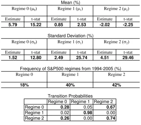
and Table 2 show that the return pattern of the S&P 500 could be easily captured with three regimes, where up-market regime has a mean of 5.79% and a relatively low volatility 1.52%. The normal regime has a mean of 0.85% and a volatility of 2.49%. The down-market regime captures market downturns and has a mean of -2.02% and a volatility of 4.51%.
calculation, volatility spillover and contagion among markets. Moreover, regime-switching models have been successfully applied to constructing trading rules in equity markets (Hwang and Satchell (2007), equity and bond markets (Brooks and Persand (2001)), and foreign exchange markets (Dueker and Neely (2004)). Chan et al. (2005) apply regime-switching models to the CSFB/Tremont hedge fund indexes to analyze the possibility of switching from a normal to a distressed regime in the hedge fund industry. The implementation of the regime-switching methodology is similar in spirit to ours; however, in our paper we propose a regime-switching beta model to measure the exposure of hedge fund indexes to different regimes that characterize market risk factors. Such exposure cannot be measured with the simple regime-switching model used by Chan et al. (2005) because this model does not account for market risk factor regimes.
Our approach maintains the spirit of Fung and Hsieh (1997) and Agarwal and Naik (2004), but we differ from these studies in the focus of our investigation. Specifically, rather than using ABS factors to capture dynamic strategies, we allow for dynamic factor loadings with different betas, where factor loadings are endogenously determined. In this way we capture, with a formal model, the idea of Fung and Hsieh (1997) to separate factors into different quintiles based on historical performance and try to access the exposure of hedge fund returns to factors in each of the quintiles. However, the use of quintiles implies the exogenous definition of states. Rather, we let the model to determine the states. Our analysis shows that hedge fund exposure to risk factors is related to a mixture of strategies based on options. The framework is also flexible, as we do not need to define a priori the strategy that hedge funds may follow, but in line with the classical Sharpe-style analysis approach (Sharpe, (1992)), the data highlight the dynamic exposure to risk factors. Therefore, we have different factor loadings for hedge fund strategies during different market regimes.
Our analysis confirms that hedge funds change their exposure based on different market conditions. Bollen and Whaley (2007) show that allowing for switching in risk exposure is essential when analyzing hedge fund performance. We show that the exposures change over time for all strategies, confirming the time-varying risk exposure of hedge funds. Factor loadings with respect to systematic risk factors vary in different regimes for almost all hedge fund indexes, validating the non-linear exposure to the market risk factor. We find that in many cases (i.e, emerging markets, distressed, event driven multi-strategy and risk arbitrage strategies) hedge fund exposure to the S&P 500 in the down-state of the S&P 500 is greater than in the normal state of the market. Moreover, our framework can capture the phase-locking property of hedge funds introduced by Chan et al. (2005).2 For example, we observe
2The term “Phase-locking” behavior is borrowed from the natural sciences, and refers to a state in which
that for all strategies in the normal market regime, factor loadings are very low or zero for some particular risk factors, including the S&P 500; however, factor loadings become very large in the down-market or up-market regimes.
Our model is able to capture changes in factor loadings depending on the volatility of the market and exposure to risk factors that, for a certain period of time, are negligible and are not captured by linear models. More specifically, we find that exposures to Large-Small (Fama-French Factor), Government Credit, and MSCI Emerging Market Debt are mostly characterized by zero or small exposure during the normal state and significant exposure during market downturns. Moreover, our results show that risk factor exposures conditional on market regimes are quite different among hedge fund indexes.
The above results suggest, first, that by using regime-switching models investors can identify and select hedge funds and hedge fund indexes with favorable market exposure in each regime and in particular in market downturns. They will also be more informed about transition probabilities between different regimes and probabilities of being exposed to several market factors.
Second, our results suggest that the common exposures of different hedge fund indexes to risk factors in the down-state of the market are the exposure to the Large-Small risk factor (which may potentially capture liquidity risk in line with Acharya and Pedersen (2005)), Credit Spread (i.e., credit risk) and change in VIX. This suggests the possibility of a sys-tematic risk among the hedge fund family that is not generated by direct market exposure. The systematic risk is attributed to liquidity and credit risks, two typically non-linear phe-nomena, and is more relevant during market downturns that are usually characterized by large volatility. This aspect is important for regulators who would like to access systematic exposure of hedge funds.
Third, our analysis shows that the idiosyncratic risk factor of hedge funds is largely characterized by changes from a low volatility regime to a high volatility state that are not directly related to market risk factors. We further explore the probability that all hedge fund strategies exhibit idiosyncratic risk in a high volatility regime. This could be interpreted as a proxy measure for contagion between different hedge fund strategies. Specifically, we calculate the joint probability of being in a high volatility state for all hedge funds. We find that the joint probability jumps from approximately 0% in May 1998 to 4% in June 1998 to 13% in July 1998 to 96% in August 1998, the month of the Long-Term Capital Management (LTCM) collapse. It started to subside in October 1998. The peak in the joint probability coincides with the liquidity crisis precipitated by the collapse of the LTCM. The results suggest that the LTCM crisis not only affected market risk factors, but also, after controlling for market and other factor exposures, affected idiosyncratic volatility of
hedge funds. This provides evidence that even after accounting for market and other factor exposures, the LTCM crisis precipitated contagion across the hedge fund industry.
Robustness analysis and out-of-sample forecasting experiments confirm the economic importance of accounting for the presence of market regimes for determining hedge fund risk exposure.
The rest of the paper is organized as follows. In Section 2 we develop a theoretical framework and define a series of beta regime-switching models that can be used to analyze different hedge fund style indexes. Section 3 describes data and presents results for the one-factor and multifactor beta regime-switching models. Section 4 presents analysis on omitted factors. Section 5 presents analysis on evolution of the idiosyncratic risk factor. Section 6 provides robustness checks. We compare our approach to OLS, asymmetric beta and threshold models. We also adjust for potential illiquidity and smoothing in the data and check that regime-switching approach is applicable to individual hedge funds as well as indexes. Section 7 conducts an out-of sample analysis. Section 8 concludes.
2
Theoretical Framework
Linear factor models such as the capital asset pricing model (CAPM) and the arbitrage pricing theory (APT) have been the foundation of most of the theoretical and empirical asset pricing literature. Formally, a simple one-factor model applied to hedge fund index returns could be represented as:
Rt =α+βIt+ωut (1)
where Rt is the return of a hedge-fund index in period t,It is a market factor, for example,
the S&P500 in period t, and ut is IID.
In this model, we can identify the exposure of hedge fund returns to a factor I. Unfor-tunately this theory constrains the relation between risk factors and returns to be linear. Therefore it cannot price securities whose payoffs are nonlinear functions of the risk factors, i.e., hedge fund returns that are characterized by the implementation of dynamic strategies. For this reason we propose a more flexible and complete model for capturing this feature: a regime-switching model.
A Markov regime-switching model is one in which systematic and un-systematic events may affect the output due to the presence of discontinuous shifts in average return and
volatility. The change in regime should not be regarded as predictable but rather as a random event.
More formally, the model could be represented as:
Rt = α+β(St)It+ωut (2)
It = µ(St) +σ(St)²t (3)
whereSt is a Markov chain withnstates and transition probability matrix P. Each state of
the market indexI has its own mean and variance. Hedge fund mean returns are related to the states of the market index and are defined by the parameter α plus a factor loading,β, on the conditional mean of the factor. Hedge fund volatilities are also related to the states of the market index I and are defined by the factor loading, β, on the conditional volatility of the factor plus the volatility of the idiosyncratic risk factor ω.3 In both cases β could be
different conditional on a state of the risk factor I.
For example, ifn = 3 (state labels are denoted as 0, 1 or 2), the model can be represented as follows: Rt= α+β0It+ωut if St= 0 α+β1It+ωut if St= 1 α+β2It+ωut if St= 2 (4)
where the state variable S depends on time t, and β depends on the state variable:
β(St) = β0 if St= 0 β1 if St= 1 β2 if St= 2 (5)
and the Markov chain St (the regime-switching process) is described by the following
tran-sition probability matrix P:4
3In all Markov states, we assume normality of the error terms and homoskedasticity within regimes.
These hypotheses are not at all restrictive since, as it will be clear in the Section 3.2.1 and Figures 1 and 2, the resulting return distributions are non-normal and heteroskedastic.
4P
P= p00 p01 p02 p10 p11 p12 p20 p21 p22 (6)
with p02 = 1−p00−p01, p12 = 1−p10−p11 and p22 = 1−p20−p22. The parameters p00,
p11 and p22 determine the probability of remaining in the same regime. This model allows
for a change in variance of returns only in response to occasional, discrete events. Despite the fact that the state St is unobservable, it can be statistically estimated (see for example
Hamilton (1989, 1990)).
Our specification is similar to the well-known “mixture of distributions” model. However, unlike standard mixture models, the regime is not independently distributed over time unless transition probabilitiespij are equal to 1/n, wheren is the number of states. The advantage
of using a Markov chain as opposed to a “mixture of distributions” is that the former allows for conditional information to be used in the forecasting process. This allows us to: (i) fit and explain the time series, (ii) capture the well known cluster effect, under which high volatility is usually followed by high volatility (in the presence of persistent regimes), (iii) generate better forecasts compared to the mixture of distributions model, since regime-switching models generate a time-conditional forecast distribution rather than an unconditional forecast distribution, and (iv) provide an accurate representation of the left-hand tail of the return distribution, as the regime-switching approach can account for “short-lived” and “infrequent” events.5
Moreover, our formal model allows us to make dynamic forecasts. More specifically, once parameters are estimated, the likelihood of regime changes can be readily obtained, as well as forecasts of βt itself. In particular, because the k-step transition matrix of a
Markov chain is given by Pk, the conditional probability of the regime S
t+k given date-t data Rt ≡ (Rt, Rt−1, . . . , R1) takes on a particularly simple form when the number of
5The Markov switching model is more flexible than simply using a truncated distribution approach, as
at each time t, we have a mixture of one or more normal distributions, and this mixture changes every
time. Using the truncated distribution will lead to a non-parametric estimation, where the down-state of the market is exogenously imposed, and it is hard to make inferences about beta forecast and conditional expectations. Instead, we use a parametric model to help us separate the states of the world. We are able to infer time-varying risk exposures of hedge funds, make forecasts, calculate transition probabilities from one state to another and calculate conditional expectations.
regimes is 2 (regime 0 and 1): Prob (St+k= 0|Rt) = π1 + (p00−(1−p11))k · Prob (St= 0|Rt)−π1 ¸ (7) π1 ≡ (1−p11) (2−p00−p11) (8)
where Prob (St = 0|Rt) is the probability that the date-t regime is 0 given the historical
data up to and including date t (this is the filtered probability and is a by-product of the maximum-likelihood estimation procedure). More generally, the conditional probability of the regime St+k given date-t data is:
Prob (St+k = 0|Rt) = Pk0at (9)
at =
·
Prob (St = 0|Rt) Prob (St= 1|Rt) ..Prob (St=n|Rt)
¸0
(10)
Using similar recursions of the Markov chain, the conditional expectation of βt+k can be
readily derived as:
E[βt+k|Rt] = a0tPkβ (11)
β ≡ [ β0 β1 ..βn]0 (12)
Time-varying betas can be easily determined by using equation 11 and setting k=0. This gives us the framework for analyzing time-varying risk exposures for hedge funds for different factors. Moreover, this framework can be used to calculate expected time-varying risk exposures for hedge funds for various factors, by setting k to be more than 0. For example, if k=1, we can calculate the evolution of expected one-month beta exposures to different factors.
The model described in equations 2 and 3 could be extended in several ways. For example, we propose a regime-switching model with non-linearity in the volatility of residuals and in
the intercept coefficient:
Rt = α(Zt) +β(St)It+ω(Zt)ut (13)
It = µ(St) +σ(St)²t (14)
In this model, additional non-linearities are captured by the intercept and residuals. Ztis
another Markov chain which proxies for all other non-linearities not captured by non-linear relationship between a particular hedge fund (index) and the risk factor I.
Usually more than one factor affects hedge fund returns. Our regime-switching beta model could be easily extended to a multifactor model.
The first extension is a model in the same spirit as the model developed by Agarwal and Naik (2004) with a non-linear exposure to the S&P 500 and a linear exposure to other risk factors. More formally:
Rt = α(Zt) +β(St)It+ K X k=1 θkFkt+ω(Zt)ut (15) It = µ(St) +σ(St)²t (16)
where θk is the linear factor loading of the hedge fund index on the k-th risk factor and Fkt
is the return on the k-th risk factor at time t.
However, this model does not consider the possibility that the exposure to other risk factors could be affected by the regime that characterizes the S&P 500. To capture this feature, we propose a multifactor beta switching model with non-linearity in residuals:
Rt = α(Zt) +β(St)It+ K X k=1 θk(St)Fkt+ω(Zt)ut (17) I1t = µ(St) +σ(St)²t (18)
This model allows us to detect the exposure of hedge fund indexes to different factors conditional on the state that characterizes the market index factor that in our empirical analysis is represented by the S&P 500.
Goodness-of-fit for our non-linear models is measured using McFadden’s (1974)
pseudo-R2 approach. In this approach, the unrestricted (full model) likelihood L
the restricted (constant only) likelihood LR as follows:
P seudo−R2 = 1− logLU R logLR
(19)
Pseudo-R2 measure has also been used by Boyson, Stahel and Stulz (2006) to compare
different hedge fund risk models. The ratio of the likelihoods measures the level of improve-ment made by the unrestricted model with respect to the restricted model. A likelihood falls between 0 and 1, so the log of a likelihood is less than or equal to zero. If a model has a very low likelihood, then the log of the likelihood will have a larger magnitude than the log of a model with high likelihood. A small ratio of log likelihoods indicates that the unrestricted model has a far better fit than the restricted model. The pseudo-R2 measures
an improvement of the unrestricted model with respect to the restricted model. Thus, when comparing two models on the same data, McFadden’s pseudo-R2 is higher for the model
with the greater likelihood. However, even though it ranges from 0 to 1 with higher values indicating a better model fit, pseudo-R2 is not a measure of explained variability, which is
captured by a classical OLS R2.
3
Empirical Analysis
3.1
Data
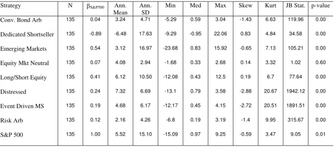
For the empirical analysis in this paper, we use aggregate hedge-fund index returns from the CSFB/Tremont database from January 1994 to March 2005. For out-of-sample analysis, we extend the dataset until October 2006. The CSFB/Tremont indexes are asset-weighted indexes of funds with a minimum of $10 million of assets under management, a minimum one-year track record, and current audited financial statements. An aggregate index is computed from this universe, and 10 sub-indexes based on investment style are also computed using a similar method. Indexes are computed and rebalanced on a monthly frequency and the universe of funds is redefined on a quarterly basis. We use net-of-fee monthly excess return (in excess of LIBOR). This database accounts for survivorship bias in hedge funds (Fung and Hsieh (2000)). Table 1 describes the sample size,β with respect to the S&P 500, annualized mean, annualized standard deviation, minimum, median, maximum, skewness and kurtosis for monthly CSFB/Tremont hedge-fund index returns as well as for the S&P 500.
For our empirical analysis, we evaluate the exposure of hedge fund indexes to the mar-ket index, the S&P 500; therefore, we concentrate only on hedge fund styles that either directly or indirectly have S&P 500 exposure. For example, we concentrate on directional strategies such as Dedicated Shortseller, Long/Short Equity and Emerging Markets as well as non-directional strategies such as Distressed, Event Driven Multi-Strategy, Equity Market Neutral, Convertible Bond and Risk Arbitrage.
Categories greatly differ. For example, annualized mean of excess return for the Dedi-cated Shortseller category is the lowest: -6.48%, and the annualized standard deviation is the highest at 17.63%. Distressed has the highest mean, 7.32%, but relatively low standard deviation: 6.69%. The lowest annualized standard deviation is reported for the Equity Mar-ket Neutral strategy at 2.94% with an annualized mean of 4.08%. Hedge fund strategies also show different third and fourth moments. Specifically, non-directional funds such as Event Driven Multi-Strategy, Risk Arbitrage and Convertible Bond Arbitrage all have negative skewness and high kurtosis. The exception is the Equity Market Neutral strategy, which has a low positive skewness and kurtosis. Directional strategies such as Dedicated Short-seller, Long/Short Equity have positive skewness and small kurtosis. Emerging Markets has a slight negative skewness of -0.65 and a small kurtosis. The market factor is characterized by high annualized excess return of 5.52% and high standard deviation of 15.10% during our sample period. Moreover, the distribution of the market factor is far from normal and is characterized by negative skewness.
3.2
Beta Regime-Switching Models
In the following sub-sections, all switching regime models have been estimated by maximum likelihood using the Hamilton’s filter and the econometric software GAUSS.
Because of the limited dataset, we prefer to adopt a two-step procedure. We first char-acterize the S&P 500 behavior by a switching-regime model and then, conditional on this result, we estimate our one-factor and multi-factor models.
Finally, in all our estimations we compute the robust covariance matrix estimator (often known as the sandwich estimator) to calculate the standard errors (see Huber (1981) and White (1982)). The estimator’s virtue is that it provides consistent estimates of the covari-ance matrix for parameter estimates even when a parametric model fails to hold, or is not even specified. In all tables we present the t-statistics obtained with the robust covariance matrix estimators, which allows us to take into account a possibility that data may deviate to some extent from the specified model.6
3.2.1 S&P 500 regimes
In this section we first verify the presence of the S&P 500 regimes in the data, and then analyze the exposure of different hedge fund indexes to the different states of the S&P 500 market index by implementing the model described in equation 3.
In order to determine the number of regimes used in the estimation, we estimated and tested models with different number of regimes and ultimately decided that using three regimes is optimal for our analysis. Using three regimes is also consistent with the literature that well recognizes the presence of normal, rolling-up or downturn regions in the returns of the equity market.78 The results of the estimation are shown in Table 2.
[INSERT Table (2) about here]
Table 2 shows that the return pattern of the S&P 500 could be easily captured with three regimes, where regime 0 has a mean of 5.79% and a relatively low volatility of 1.52%. We denote this regime as the up-market state, which has a very low probability of remaining in the same regime in the following month: P00=28%. Regime 1 has a mean statistically
different than zero and equal to 0.85% and a volatility of 2.49%, and we call it a normal state. This is a persistent regime, and the probability of remaining in it is 98%. The last regime captures market downturns and has a mean of -2.02% and a volatility of 4.51%. The probability of remaining in this regime is 74%.
The model estimation allows us to infer when the S&P 500 was in one of the three regimes for each date of the sample using the Hamilton filter and smoothing algorithms (Hamilton, 1994).
We observe that in the first part of the sample, the S&P 500 returns are frequently characterized by the normal regime 1, in particular from July 1994 to December 1996 (91.7% of time in normal regime and 8.3% in the market downturn). The period from 1997 through 2003 is characterized primarily by two other regimes: up-market (30.4%) and down-market (64.6%). This outcome is generated mainly by high instability of the financial markets starting from the Asian down-market in 1997, well captured by regime 2, the technology and internet boom, well captured by regime 0, the Japanese down-market of March 2001, September 11, 2001 and the market downturn of 2002 and 2003, captured mostly by regime 2. The last part of the sample from 2003 through 2005 is characterized by the normal regime
estimator and the robust covariance matrix estimator are similar.
7All switching regime models have been estimated by maximum likelihood using the Hamilton’s filter and
the econometric software GAUSS.
8Goetzmann et al. (2007) show that an optimal strategy for hedge funds might be selling
out-of-the-money puts and calls, ensuring that during normal regimes, hedge fund managers obtain a positive cash flow, and have a large exposure in extreme events.
1 (100%). It is important to note that the three-regime approach does not imply simply splitting the data sample into large negative, large positives or close to the mean returns. The regime approach allows us to capture periods where the return distribution belongs to large volatility periods characterized by large downturns or more tranquil periods. In all these different regimes we may face positive or negative returns.9
In addition to analyzing the change in the S&P 500 returns, and probability of being in a particular regime, we derive both conditional and unconditional distributions for the S&P 500 for all three regimes as well as for the total time series.
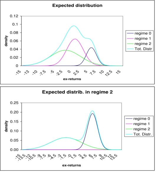
[INSERT Figure (1) about here]
Figure 1 depicts unconditional distributions of the S&P 500 overall, in down-market, normal and up-market regimes. First, it is worthwhile to note that during the time period analyzed in the paper, the market clearly experienced three distinct regimes: up-market, normal and down-market. Moreover, the total distribution is skewed, and distribution of being in a down-market state is characterized by fat tails. Figure 1 also depicts conditional distributions of different regimes, conditional on starting in regime 2, a down-market regime. The resulting total distribution closely overlaps regime 2 distribution, especially in the left tail. Therefore, once in down-market, the market is more likely to stay in down-market (74%), and both conditional regime 2 and total distribution are fat-tailed.
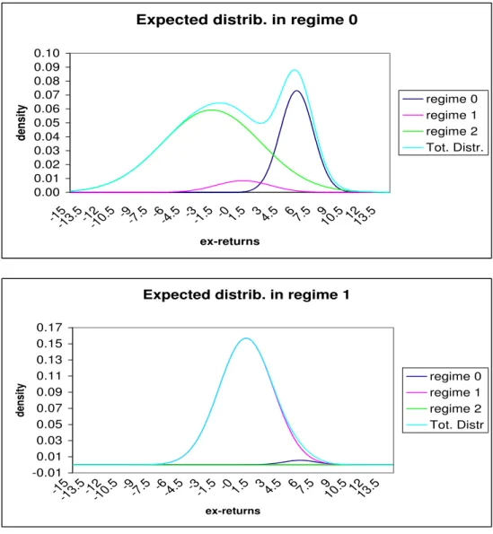
[INSERT Figure (2) about here]
Figure 2 shows conditional distributions of the S&P 500 overall, in down-market, normal and up-market regimes first conditional on an up-market regime and second conditional on a normal regime. Interestingly, conditional on being in an up-market, there is a certain probability of staying in an up-market (28%), but there is also a large left-tail probability of moving to a down-market (67%). It looks like the up-market regime is often transitory, frequently followed by a down-market regime. Conditional on being in a normal regime, the total distribution is almost identical to the conditional probability of a normal regime. Therefore, if a market is in the normal regime, it is more likely to be persistent (98%). The conditional distributions for all regimes are very close to normal in this case. Nevertheless, there is a small probability of 2% of moving to an up-market regime that is more likely (67%) followed by a down-market.
9This approach is closely compared to an alternative threshold approach where a sample is split into
positive and negative returns, following Fung and Hsieh (1997). These two approaches are carefully compared in Section 6. More specifically, the regime-switching approach allows us to endogenously determine changes in market return distributions without exogenously splitting the data into positive and negative returns.
Overall, the results confirm that during the period of January 1994 to March 2005, the S&P 500 was clearly characterized by three separate regimes. In the paper, we are interested in clearly understanding the exposure of each hedge fund strategy to the market in all these regimes. In other words, we are interested in finding the exposure of hedge fund returns to all parts of this distribution. Using the results in Figures 1 and 2, it is clear that not accounting for three separate regimes and only concentrating on a normal regime will underestimate the left tail of the distribution and thus bias hedge fund market risk exposure.
3.2.2 One-factor model
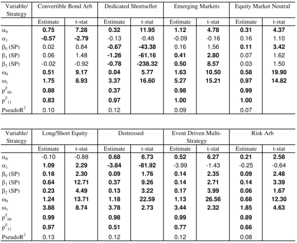
After having characterized the process for the S&P 500, we analyze the exposure of different hedge fund strategies to different S&P 500 regimes. The analysis is based on the model presented in equation 13 and results are shown in Table 3.
[INSERT Table (3) about here]
We find different factor loadings with respect to the S&P 500 regimes for almost all hedge funds indexes. The only exception is the Convertible Bond Arbitrage strategy. Regarding the more directional strategies (Dedicated Shortseller and Long/Short Equity), we do find significant exposures to the S&P 500 regimes, but the factor loadings vary a lot for different regimes. In particular, Dedicated Shortseller shows a large negative exposure of -1.26 to the S&P 500 in normal times. This relationship is maintained for the down-market period; however, the exposure is reduced in half for the up-market state of the market. Long/Short Equity strategy aims to go both long and short on the market during the normal regime. Our analysis shows that the exposure to the market during the normal regime is three times as high as the exposure during the other two regimes. There is, therefore, an attempt of this strategy to reduce the exposure to the market downturns, but the exposure remains still positive, as shown in Table 3.
The Emerging Markets strategy shows a peculiar positive exposure mostly when the market is characterized by the down-market state and is relatively large in normal time. A potential explanation of this large exposure in market downturns can come from the fact that many emerging markets do not allow short-selling and lack availability of option instruments to be used for hedging. Therefore, the exposure result for the Emerging Markets strategy is similar to writing a put option on the S&P index.
For Equity Market Neutral we find a positive exposure in regime 0, i.e., when the market is rolling up. The exposure is zero in normal times and when the market is mostly charac-terized by a downturn. This result is in line with the fact that the Market Neutral strategy
can neutralize the effects of normal movements of the market, but when the market is sud-denly moving to another regime facing a phase-locking phenomenon, the exposure becomes positive.
The other three strategies are related to the Event Driven categories. The exposures to the S&P 500 are positive and quite similar in different states of the market, especially for the Event Driven Multi-Strategy, which has a slightly higher exposure during the market downturn. Distressed security strategy presents a larger exposure in normal times. The Risk Arbitrage Strategy presents a positive exposure in the normal regime and when the market is rolling up and an almost zero exposure in the down-market regime.
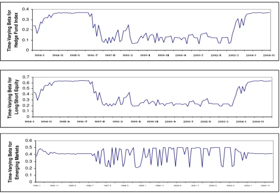
In addition to showing that hedge fund exposure differs over various market regimes, a regime-switching framework allows us to calculate time-varying risk exposure of hedge funds implied by the data, i.e., time-varying betas with respect to various factors including the S&P 500 for various hedge fund strategies. Time-varying betas can be easily determined using equation 11 by assuming that k=0. This gives us the framework for analyzing time-varying risk exposures for hedge funds for different factors. Time-time-varying market risk betas are depicted for several hedge fund strategies in Figure 3.
[INSERT Figure (3) about here]
First, note that the market exposure changes over time for all strategies, confirming that hedge funds are implementing dynamic strategies. Figure 3 depicts the evolution of market betas for Hedge fund index, Long/Short Equity and Emerging Markets strategies. For the Hedge fund index and Long/Short Equity strategy, starting the middle of 2003, market exposure dramatically increased. For example, for the Combined Hedge fund index, the forecasted exposure in April 2003 was 0.07, seemingly market-neutral; however, exposure in March 2005 increased to 0.37, which is a significant positive market exposure. For the same time period, the exposure of the Long/Short Equity increased from 0.20 to 0.64, more than 3-fold.10 It is interesting to note that in all these categories, the market beta is cyclical:
it was increasing from 1994 through 1997, then it abruptly dropped and stayed low for 7 years, and started to increase in 2003. Similar behavior is also observed for Convertible Bond Arbitrage, Risk Arbitrage, Distressed, and Dedicated Shortseller (for this strategy, the exposure is increasing in the negative direction). This cyclical behavior in market beta can be largely attributed to the changes in market regimes over this time period.11
10Long/Short Equity strategy comprises majority of hedge funds represented in the Combined Hedge fund
index.
11As stressed above, our analysis shows that in the first part of the sample, from July 1994 to December
When volatility of the S&P 500 is high between 1997 and 2003, hedge funds in these strategies on average decrease their exposure to the market and increase when volatility of the market subsides (normal regime). Therefore, on average, when market volatility is high and changing, hedge funds reduce exposure.
On another hand, time-varying beta for the Emerging Markets category shows a different story. For the Emerging Markets category, from 1997 to 2003, the exposure fluctuates a lot, from 0.2 to 0.5. However, from the beginning of 2003 to the end of the data sample, the market exposure equilibrates at 0.41. The similar behavior is observed for Equity Market Neutral strategy and for the Event Driven Multi-Strategy.
In summary, hedge fund exposure depends on volatility regimes of the S&P 500. More-over, the exposure to the S&P 500 index changes through time. Therefore, investors should take into account change in market volatility and how it affects hedge fund risk. Regulators should do stress testing with different market conditions and consider the implications for hedge fund behavior. This will contribute to the analysis of systemic risk.
This framework can be extended to calculating expected hedge fund exposures to different factors one month from now, 6 months from now, 1 year from now and so on. Our flexible approach allows us to calculate expected time-varying betas for t + k periods by using specification 11.
Idiosyncratic risk presents different levels of volatility. Convertible Bond Arbitrage, Eq-uity Market Neutral and Risk Arbitrage tend to have relatively low values of idiosyncratic volatility for both volatility regimes. The idiosyncratic volatility in the high volatility regime is always less than 2% for these strategies (Table 3). However, for the other five strategies, in both regimes, the idiosyncratic volatility is relatively high. The average idiosyncratic volatil-ity for a high volatilvolatil-ity regime for these strategies is about 4% at the monthly level. More-over, high volatility regimes are persistent. This is more evident for Dedicated Shortseller, Emerging Markets, Equity Market Neutral and Long/Short Equity strategies. Controlling for idiosyncratic risk is important for investors in terms of portfolio risk and diversification, and for regulators in controlling spill-over effects that can propagate from the hedge fund idiosyncratic risk.
Nevertheless, other risk factors play a role as important as the S&P 500 in characterizing the time-varying hedge fund exposure. This aspect is investigated in the next section with a multifactor model.
through 2003 is characterized primarily by two other regimes: up-market and down-market. The last part of the sample from 2003 through 2005 is characterized by the normal regime.
3.2.3 Multifactor model
Multifactor model with non-linear exposure only to the S&P 500
As discussed above, other factors affect hedge fund index returns, and this calls for the use of a multifactor framework. We begin with a comprehensive set of risk factors that will be candidates for each of the risk models, covering stocks, bonds, currencies, commodities, emerging markets, momentum factor and volatility. These factors are presented in Table 4. They are also described by Chan et al. (2005) as relevant factors to be used for each hedge fund strategy. Given the limited dataset, we use a step-wise approach to limit the final list of factors for our analysis. Employing a combination of statistical methods and empirical judgement, we use these factors to estimate risk models for the 8 hedge fund indexes. In all our analyses, hedge fund returns, S&P 500, USD, Lehman Government Credit, Gold, MSCI Emerging Markets Bond Index, MSCI Emerging Markets Stocks Index and Momentum French factor are used in excess of LIBOR returns.
[INSERT Table (4) about here]
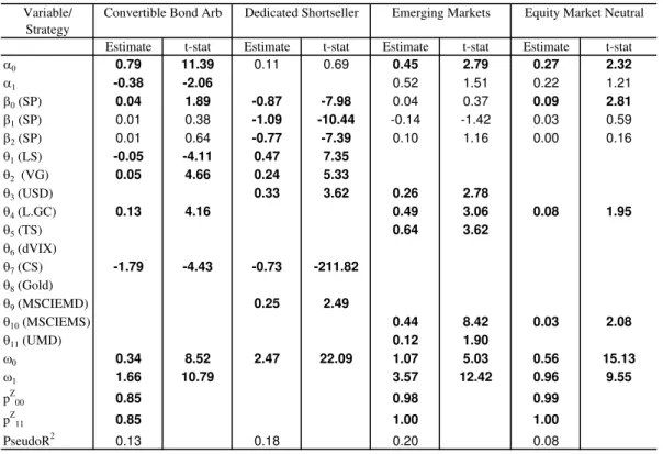
We first consider the model presented in equation (15) and the results for this model are contained in Table 5. Here, we are considering linear factors: Large-Small, Value-Growth, USD, Lehman Government Credit, Term Spread, change in VIX, Credit Spread, Gold, MSCI Emerging Markets Bond Index, MSCI Emergent Markets Stock Index, Momentum French factor and non-linear exposure to different states of the S&P 500.12
[INSERT Table (5) about here]
The number of factors F selected for each risk model varies from a minimum of 2 for Equity Market Neutral to a maximum of 8 for the Event Driven Multi-Strategy, not including the S&P 500 index. This pattern is plausible because the Event Driven Multi-Strategy by definition includes a broad set of strategies; hence a broad array of risk factors is needed to capture the variation in this category versus other categories.
The statistical significance of the factor loadings on the S&P 500 conditional on the different regimes is almost the same as the one obtained in the previous analysis with only the S&P 500 risk factor. The only main difference is the exposure of the Distressed strategy
in the up-market state to the S&P 500 and the exposure of the Emerging Markets strategy in the up-market and normal states to the S&P 500. This indicates that the analysis performed above is robust to the inclusion of other factors that may affect hedge index returns.
Regarding the Large Minus Small factor, we observe that this factor is relevant for almost all hedge fund strategies, the only exceptions are Equity Market Neutral and Emerging Markets strategies. The exposure to the Large Minus Small factor is negative for almost all hedge funds indexes (the only exception is the Dedicated Shortseller) suggesting that returns of these hedge indexes resemble those achieved by going long on small stocks and short on large stocks (as shown previously by Agarwal and Naik (2004) and Chan et al. (2005)). Another potential explanation is that this factor is capturing liquidity risk as highlighted by Amihud (2002) and Acharya et al. (2004). We consider this aspect later.
The hedge fund exposure to Value Minus Growth factor is positive for Convertible Bond Arbitrage, Dedicated Shortseller, Distressed, Event Driven Multi-Strategy and Risk Arbi-trage.13
Credit spread is a common negative factor for five out of eight strategies. This is of great importance for regulators who are concerned about common risks among hedge funds. This is particulary relevant given the recent credit crisis and its effect on hedge funds (August 2007).
Change in VIX is only significant for 2 strategies. This is surprising given that hedge funds take bets on volatility. There could be two complementary reasons for this: (1) Switching in S&P 500 regimes based on mean and volatility already captures this exposure, and (2) Hedge funds take non-linear bets in volatility and thus the current linear change in VIX exposure does not capture the true underlying non-linear exposure. However, if the first reason were the only true reason, then change in VIX will be captured by OLS; however, it is not as will be shown in the robustness analysis. Therefore, later in the paper we introduce models with omitted factors to capture non-linearity in VIX exposure.
A detailed analysis of other factors is presented in Appendix 1 for each hedge fund strategy. The list of factors and hedge fund exposures to these factors is unique for each strategy; therefore, we are analyzing them one by one for each strategy.
Multifactor model with non-linear exposure to all factors
Finally, we estimate the multifactor model specified in equation (17) and the results are contained in Table 6. Here, we are considering non-linear exposure to factors: S&P 500,
13We also consider Fama and French “size” and “book-to-market” risk factors (Fama and French, 1993)
and the results are similar. We prefer to use the Large-Small and Value-Growth Russell indexes because they are investable portfolios, following Chan et al. (2005).
Large-Small, Value-Growth, USD, Lehman Government Credit, Term Spread, change in VIX, Credit Spread, Gold, MSCI Emerging Markets Bond Index, MSCI Emerging Markets Stock Index and Momentum factor. The three coefficients that we estimate for each factor represent the non-linear factor exposure of hedge fund indexes to the three states of the S&P 500. Because of the limited dataset we only consider variables that are statistically significant in the previous multifactor linear exposure analysis. Clearly, the results may depend on this choice, thus later we relax this assumption and consider the possibility of a non-linear exposure to other risk factors as well (see section 4).
[INSERT Table (6) about here]
All strategies have exposure to the S&P 500 in at least one regime even after accounting for conditional exposure to other risk factors. Generally, we find that the model that ac-counts for different factors conditional on the state of the market is richer and captures more exposures compared to previous models. Moreover, the model shows that factor exposure is changing conditional on the state of the market. Finally, this model captures more of hedge fund return variation as is evidenced by a higher pseudo-R2 for all hedge fund strategies
compared to the one-factor model and the multifactor model with non-linear exposure only to the S&P 500.
For five out of eight strategies (Convertible Bond Arbitrage, Long/Short Equity, Dis-tressed, Event-Driven Multi Strategy and Risk Arbitrage) our results suggests that hedge funds tend to hold illiquid or low-credit securities and thus are susceptible to liquidity crises.14
We find that in all of these strategies, exposure to LS (Large-Small) is negative and highly significant during market downturn. In all these cases (except Long/Short Equity) the ex-posure is higher in absolute value compared to the exex-posure to LS during the normal market conditions.15 Actually, for Convertible Bond Arbitrage, Event-Driven Multi-Strategy and
Risk Arbitrage, the exposure to LS during normal market conditions is negligible. Overall, almost all hedge fund indexes have a significant exposure to the LS factor in at least two out of three states and especially during market downturn.
Furthermore, note that LS is the only common factor in the market downturn for six out of eight hedge funds strategies and for five out of eight it has the same sign. This
14For Dedicated Shortseller the exposure to LS is positive. The strategy makes money in the down-state
of the market; therefore, the shock in the down-state will be beneficial for this strategy.
15The Long/Short Equity strategy is the only strategy compared, to the other four, which holds relatively
result suggests that this variable may potentially capture a common factor in the hedge fund industry. A potential explanation of this result is that liquidity risk is relevant for hedge funds and liquidity shocks are highly episodic and tend to be preceded by or associated with large and negative asset return shocks, whereby liquidity risk is rendered a particularly non-linear phenomenon. This result is in line with the potential interpretation of Acharya and Schaefer (2006) that the “illiquidity” prices in capital markets exhibit different regimes. In a normal regime, intermediaries, including hedge funds, are well capitalized and liquidity effects are minimal. In the “illiquidity” regime usually related to market downturns, intermediaries are close to their risk or collateral constraints and there is a “cash-in-the-market” pricing (Allen and Gale (1994, 1998)). In this framework, hedge funds, which often invest in derivatives and complex structured products, are more likely to be the marginal price setters and therefore more largely affected by the “illiquidity” regime.
Moreover, we find that another common risk factor for hedge funds is Credit Spread, especially the effect of the Credit Spread in the negative states of the market. For most of the strategies (Convertible Bond Arbitrage, Equity Market Neutral, Long/Short Equity, Distressed and Event-Driven Multi Strategy), the impact of the Credit Spread in the down-market regime on hedge fund index returns is negative.16 The credit risk in the down-state
of the market is the most important risk factor that should be controlled by regulators. Moreover, credit spread can also serve as a proxy for illiquidity risk. When credit spread increases, cost of capital increases and investors prefer to invest in more liquid and high-quality instruments. Therefore, low-credit illiquid investments suffer.
Furthermore, our analysis shows that many factor exposures are characterized by the phase-locking property. For example, the exposure to the S&P 500 is negligible during normal states of the market for the Convertible Bond Arbitrage, Equity Market Neutral, Event Driven Multi-Strategy and Risk Arbitrage, but changes to positive in up- and down-states of the market. Also, the exposure to Lehman Government Credit is negligible for Convertible Bond Arbitrage, Emerging Markets and Long/Short Equity indexes; however, it becomes highly positive and significant for up- and down-market states. The exposure to UMD is negligible in the normal state of the market for Emerging Markets, Long/Short Equity and Event Driven Multi-Strategy, but becomes highly positive and significant in the up- and down-states.
Nevertheless, the phase-locking phenomenon could be produced by dynamic strategies and/or a factor exposure of hedge fund asset portfolio that becomes statistically relevant only in certain states. With our approach we are not able to distinguish among the two
16The introduction of CS for the Equity Market Neutral strategy is in Section 4 and in Table 7 where we
phenomena and simply capture the total exposure that arises from both dynamic strategies and asset portfolio non-linear exposures.
In Appendix 2 we consider each strategy separately and address time-varying risk expo-sures for various factors.
As a robustness check, we test whether statistically significant coefficients are also statis-tically different from each other. We investigate this aspect for different hedge fund indexes, and indeed for some coefficients we cannot reject the hypothesis that they are equal. Never-theless, even if some of the estimated coefficients are similar, we are able to find that some of them are statistically equal only in two of the three states. This confirms that factor exposures change conditional on different states.
It is important to underline that our results may suffer due to data limitation. How-ever, we still find convincing evidence that factor exposures are different for various factors conditional on the state of the market and for different hedge fund indexes. Moreover, the model shows that factor exposure is changing conditional on the volatility of the market risk factor. This confirms our initial hypothesis that the exposures to different risk factors are time-varying and conditional on the state of the market risk factor. Indeed, for many factors we observe that the risk exposure is zero during normal times, and suddenly becomes positive or of opposite sign during market downturns characterized by high volatility.
4
Omitted Factors
The step-wise linear approach was used to limit the final list of factors for the analysis in the multifactor models with linear and non-linear exposures (Tables 5 and 6). However, the step-wise linear analysis uses linear models and might miss several risk factors that can impact the return profile of hedge fund strategies.
Specifically, the step-wise linear analysis could miss exposures that are only present during market downturns, exposures related to liquidity events and low-probability events or exposures with different signs for different regimes. In this section we attempt to account for the omitted factors and perform several analyses of potential non-linear risk exposures not highlighted in previous sections. Specifically, we are considering factors that were originally eliminated by the step-wise linear procedure and are not considered in Tables 5 and 6.
Our analysis in Table 7 shows that the change in VIX is an omitted factor for most of the strategies. For these strategies VIX is important, as the return process of these strategies is related to market volatility. For example, convertible bonds contain imbedded equity call
options that allow investors to convert the bonds into shares if the underlying share price rises.
[INSERT Table (7) about here]
Change in VIX is a variable that needs to be interpreted jointly with different regimes of the S&P 500. For the Convertible Bond Arbitrage strategy, the effect of Change in VIX is negative in crises markets (-0.08) and positive in up-markets (0.05).
The relationship between a convertible bond price and stock price is concave when stock price is low (down-market) and highly convex when the stock price is high (up-market). Therefore, in the up-market, we expect change in volatility to attribute to additional returns of the strategy, and in down-markets, the change in volatility negatively affects the returns of the strategy.
For Risk Arbitrage, the exposure to change in VIX is positive and significant, especially during normal periods (0.09), but negative during down-market periods (-0.12).
Risk Arbitrage strategy is concerned with the success of a merger, and increase in volatil-ity in down-times often signals an increase in probabilvolatil-ity of failure. The same applies to Distressed strategies (-0.22 in down-state and 0.24 in the normal state).
Another example is the effect of change in VIX for the Dedicated Shortseller strategy. We find that the exposure to the change in VIX is highly positive only in the negative market state (0.27), but negative in all other states (-0.42 for up-state and -0.27 for normal state). In this case the exposure to the change in VIX is opposite to the other strategies, possibly due to the nature of the strategy that profits from negative volatility shocks to the market. In all of these cases, exposures to the change in VIX have opposite signs and similar magnitudes for down and normal markets; and this is the main reason why linear factors are not able to capture this exposure.
Credit Spread and Term Spread were irrelevant factors for Equity Market Neutral strategy and were not considered in the models (Tables 5 and 6). In Table 7 we explicitly considered these factors. We find that in normal conditions, Credit Spread is irrelevant for Equity Market Neutral strategy. However, in downturns of the market, it is highly negative and significant (-1.75, t-stat: -2.39). This again confirms that credit risk is the common factor across different hedge fund strategies.
In the previous models, we found that neither LS nor change in VIX were relevant for the Emerging Markets strategy. However, after explicitly accounting for change in VIX for this
strategy, we find that change in VIX is significant for the up-market and normal regime and exposure to the LS factor is negative and significant in normal and down-market periods.
In conclusion, we find that using linear models and a step-wise linear approach of nar-rowing down significant factors misses several factors for hedge fund analysis. On average, the effect of a factor can be negligible; however, this is due to lumping the effect of the factor instead of separately calculating exposures in up-market, down-market and normal states. We find that often exposures during normal and down-markets are of opposite signs, and often, the exposures during normal states are not significant from zero. Therefore, if we do not separate the factor effects into different market regimes, we underestimate the real hedge fund exposure to this factor.
We find that change in VIX is important for hedge fund strategies, and, specifically, the exposure of hedge fund strategies to the change in VIX is non-linear and depends on the state of the market. Moreover, we find that exposures to several factors, such as LS and Credit Spread, are highly negative for most of strategies in the down-market state. We argue that this exposure could be related to liquidity risk and credit risk, but a deep analysis of this issue is needed and is left to further investigation.
5
Idiosyncratic Risk Factor
In addition to the derivation of the expected market exposures, the switching regime beta model allows us to separate and show the evolution of the idiosyncratic risk of hedge funds. In particular, our estimation of the Markov chain for the idiosyncratic risk of hedge funds shows that the idiosyncratic risk is characterized by two different regimes with high and low volatility for 6 of the 8 strategies. Exceptions are Distressed and Dedicated Shortseller, which are always characterized by a large volatility regime (idiosyncratic volatility is 1.36% for Distressed and 2.31% for Dedicated Shortseller, Table 6). These monthly volatilities are in-line with high volatility regimes for other strategies. The volatility parameters in the two volatility regimes (high and low) are largely different, and the idiosyncratic risk factor of all 6 strategies shows that the volatility in the high regime is at least twice the volatility in the low volatility regime of the idiosyncratic risk (see in Table 6 for values of $0 and $1.)
The estimated probability of switching from one regime to another is on average about 10%, but the probability of remaining in the same regime is about 90%, meaning that volatility regimes are quite persistent.
The estimations of the coefficients and the evolution of the probability of being in the high volatility regime for the idiosyncratic risk factor are similar across three models described in
equations 2, 13 and 17. This means that we are consistently estimating the idiosyncratic risk factor and it makes our results robust to different specifications. Therefore, we only depict results for the model described in equation 17.
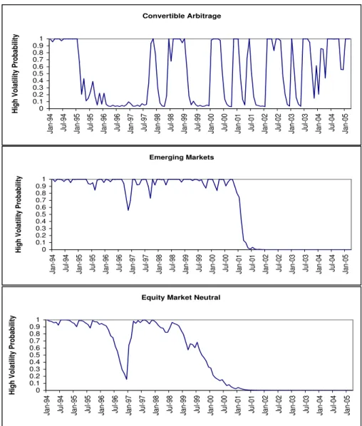
Referring to the model estimation presented in Table 6, in Figures 4 and 5 we show the evolution of the probability of being in the high volatility regime for all 6 strategies.
[INSERT Figure(4) about here]
[INSERT Figure(5) about here]
Figures 4 and 5 plot monthly probabilities from January 1994 to March 2005 of hedge fund indexes facing a high volatility regime for the idiosyncratic risk factor, i.e., volatility of the hedge fund indexes not related to the volatility of the S&P 500 index and other risk factors. We see that the evolution of the volatility of different strategies is quite different. In particular, we observe that Long/Short Equity and Emerging Markets indexes present a low probability of being in the high volatility regime in the last part of the sample and a high probability in the middle of the sample that corresponds to the series of crises and rallies from 1997 till 2001. Therefore, the risk faced by the S&P 500 already captured by the switching beta is amplified in the middle of the sample for these strategies. This indicates not only that the link with the S&P 500 is changing, but also that the idiosyncratic risk of the hedge fund indexes may switch to the high-volatility regime at the same time when the market is characterized by turbulence. This can be explained by omitted or latent variables such as idiosyncratic liquidity risk or factors that affect mostly the hedge fund industry (as in the case of LTCM default). For example, Emerging Markets, Event Driven Multi-Strategy, Long/Short Equity and Risk Arbitrage are all related to different liquidity events more or less related to the LTCM crisis.
Event Driven Multi-Strategy is almost always characterized by the low volatility regime for its idiosyncratic risk factor; however, the probability of a high volatility regime greatly increases for periods characterized by high illiquidity events and other unexpected shocks not correlated with market returns. For example, in February 1994, the U.S. Federal Reserve started a tightening cycle that caught many hedge funds by surprise, causing significant dislocation in bond markets worldwide; the end of 1994 witnessed the start of the “Tequila Crisis” in Mexico; in August 1998, Russia defaulted on its government debt and LTCM collapsed leading to a liquidity crunch in worldwide financial markets; the first quarter of
2000 saw a crash of the Internet boom, and in the middle of 2002 there was a drying out of merger activities, a decrease in defaults and the release of news about WorldCom accounting problems. During all of these periods, the probability of a high volatility regime skyrocketed, reaching 1 for the LTCM and the Russian default crisis.
The most interesting indicator is the evolution of being in the high volatility regime by the Convertible Bond Arbitrage index that indicates that the strategy has moved to a large volatility regime from the end of 2003 and is still characterized by this regime at the end of the sample considered (March 2005). If we jointly consider the state of the market index (tranquil normal period in the last two years of the sample) and the state of the idiosyncratic risk factor for the Convertible Bond Arbitrage index, we see that the switching regime beta model is able to disentangle whether the source of risk is characterized by market conditions or by potential distress in the hedge fund index strategy. Not surprisingly, April 2005 (not in the sample period) saw extremely low returns and high liquidations in the Convertible Bond Arbitrage sector. Merely tracking market exposure will not lead to this predictive result.
We further explore the probability that all hedge fund strategies exhibit idiosyncratic risk in a high volatility regime. This could be interpreted as a proxy measure for contagion between different hedge fund strategies. Specifically, we calculate the joint filtered probability of being in a high volatility state for all hedge funds and plot them in Figure 6. We find that the joint filtered probability jumps from approximately 0% in May 1998 to 4% in June 1998 to 13% in July 1998 to 96% in August 1998, the month of the LTCM collapse. It started to subside in October 1998. The peak in the joint probability coincides with the liquidity crisis precipitated by the collapse of LTCM.17 The results suggest that the LTCM
crisis not only affected market risk factors, but also, after controlling for market and other factor exposures, affected idiosyncratic volatility of hedge funds. This provides evidence that even after accounting for market and other factor exposures, the LTCM crisis precipitated contagion across the hedge fund industry. In our data, we found that this was the only case where the joint probability of being in a high volatility state for all hedge funds spiked and approached one.
[INSERT Figure(6) about here]
17We check this result against a possibility that randomly we can have all eight strategies exhibiting high
6
Robustness Analysis
6.1
Comparison with OLS Regression
In a multifactor setting, we consider the model presented in equation (15) and the results for this model are contained in Table 5.
The natural way to test the regime-switching model is to compare its results to those obtained using OLS regression. The results for the OLS regression are presented in Table 8. They are consistent, meaning, that factor loadings have the same sign in both models; however, the regime-switching model is clearly superior based on pseudo-R2 metric.18
For each hedge fund index, pseudo-R2 is larger for regime-switching models compared to
OLS models. Moreover, several estimates that are significant in the regime-switching model are not significant for the OLS model. OLS is missing some factor exposure and does not take into account time-variability of risk factors based on market conditions.
[INSERT Table (8) about here]
6.2
Asymmetric Beta and Threshold Models
An alternative way to study time-varying non-linear hedge fund exposure to market factors is through an asymmetric beta model. In this model, the distribution of Rt is truncated
either at the median or zero and betas for “up or down” markets are compared. This ap-proach has been applied to hedge funds in Agarwal and Naik (2004), Mitchell and Pulvino (2001), Asness, Krail and Liew (2004) and Chan et al. (2005). The authors found significant differences between “up” and “down” betas. Specifically, they found Event-Driven types of strategies including Risk Arbitrage, Distressed and Event-Driven Multi-Strategy exhibit zero correlation with up-market conditions, but a large positive exposure during down-market conditions. Emerging Markets strategy shows a much higher down-market correlation com-pared to up-market. Moreover, authors find that the Equity-Market Neutral strategy has a
18It is important to note that a pseudo-R2 only has meaning when compared to another pseudo-R2 of
the same type, on the same data, and predicting the same outcome. In this situation, a higher pseudo-R2
much higher up-market beta compared to the down-market beta. We replicate the analysis and find identical results in our analysis.19
We further extend the asymmetric beta model and develop a threshold model allowing for three states. Specifically, we look at asymmetric betas in hedge fund exposure by specifying different beta coefficients for down-markets, normal markets and up-markets. Specifically, consider the following regression:
Rit = αi + βi+It+ +βi0It0 + βi−It− + ²it (20) where It+ = It if It> µ+σ 0 otherwise It0 = It if µ−σ < It< µ+σ 0 otherwise It−= It if It≤µ+σ 0 otherwise (21) where It is the return on the index, µis the mean and σ is its standard deviation.
Since It = It++It0 +It−, the standard linear model in which fund i’s market betas are
identical in up and down-markets is a special case of the more general specification (20), the case whereβ+
i =βi0 =βi−. The specification (20) essentially tries to capture asymmetries in
the index exposures.
Unlike the asymmetric model, a regime-switching model allows for endogenous definition of expected returns and volatilities defined from the data. The regime-switching model also does not switch as often as the asymmetric model. Moreover, the regime-switching model may include positive returns for the down-market state and negative returns for the up-market state.
Using the specification (20), we regress hedge fund returns on the S&P 500 index dur-ing up (It+), normal (I0
t) and down (It−) conditions. The results are reported in Table 8.
Beta asymmetries are quite pronounced especially, for Emerging Markets, Distressed, Event Driven Multi-Strategy and Risk Arbitrage. For example, the Distressed index has an up-market beta of 0.07 (not significant)—seemingly up-market neutral—however, its down-up-market beta is 0.38! The exposure of the Convertible Bond Arbitrage strategy to the S&P 500 is negligible for both up and down-markets; therefore, a more comprehensive model is needed to measure the exposure of this style.
[INSERT Table (8) about here]
The results using the threshold model are similar to the ones obtained using the regime-switching methodology presented in Table 3. However, there are several numerical dif-ferences. For example, the regime-switching methodology finds that the Market-Neutral strategy has market-neutral exposure in all states except an up-market state. However, the threshold methodology finds positive market exposure in up (I+