Path Prediction using Machine
Learning
Alex Grzegorz Zyner BE (Hons 1), BSc
A thesis submitted in fulfilment of the requirements of the degree of
Doctor of Philosophy
Australian Centre for Field Robotics
School of Aerospace, Mechanical and Mechatronic Engineering The University of Sydney
I hereby declare that this submission is my own work and that, to the best of my knowledge and belief, it contains no material previously published or written by another person nor material which to a substantial extent has been accepted for the award of any other degree or diploma of the University or other institute of higher learning, except where due acknowledgement has been made in the text.
Alex Grzegorz Zyner
Autonomous vehicles are still yet to be available to the public. This is because there are a number of challenges that have not been overcome to ensure that autonomous vehicles can safely and efficiently drive on public roads. The nature of urban road-ways are particularly difficult, as they contain significant human factors that make it difficult to predict the actions of human driven vehicles. Accurate prediction of other vehicles is vital for safe driving, as interacting with other vehicles is unavoidable on public streets. This thesis explores reasons why this problem of scene understanding is still unsolved, and presents methods for driver intention and path prediction. The thesis focuses on intersections, as this is a very complex scenario in which to predict the actions of human drivers. More specifically, it focuses on intersections without traffic signals. These scenarios are significantly more difficult to predict the actions of human drivers compared to intersections with signals dictating which vehicles must give way to others.
Modern vehicle sensors are able to accurately track other vehicles at a significant distance using onboard sensors in real time. However, there is very limited data available for intersection studies from the perspective of an autonomous vehicle. In-stead, common datasets typically use overhead sensors to study ‘smart intersections’ or are limited in the quality of sensor data. This thesis presents a very large dataset of over 23,000 vehicle trajectories through five different unsignalised intersections. This dataset was collected using a lidar based vehicle detection and tracking system onboard a vehicle. Analytics of this data is presented, and these datasets are used in the training and validation of the algorithms presented in this thesis.
Even though predicting the actions of traffic is a complex and unsolved engineering problem, it must be solvable. After all, people drive vehicles safely every day in all sorts of traffic conditions. An experienced human driver has an intuition of what other vehicles are going to do, based off subtle movement cues. This thesis presents driver intention and path prediction techniques that aim to capture this intuition for use in autonomous driving. To determine the intent of vehicle at an intersection, a method for manoeuvre classification through the use of recurrent neural networks is presented. This allows accurate predictions of which destination a vehicle will take at an unsignalised intersection, based on that vehicle’s approach.
The final contribution of this thesis presents a method for driver path prediction. It produces a multi-modal prediction for the vehicle with uncertainty assigned to each mode. Given that intersections are by nature multi-modal (there are multiple ways to traverse an intersection, go straight, turn left / right), the output of this prediction algorithm is also multi-modal to match the problem space. By applying a mixture density network as the output layer to a recurrent neural network, and using full sequence to sequence training, this method produces a probability distribution of the future path of the vehicle. A presented temporal clustering method is then used to produce a multi-modal output, where each mode has its own uncertainty. In addition, these multiple outputs are ranked according to their individual probability. By using a driven approach the output modes are not hand labelled, but instead learned from the data. This results in there not being a fixed number of output modes. Whilst the application of this method is vehicle prediction, this method shows significant promise to be used in other areas of robotics.
It’s been an incredible journey. And it most certainly would not have been possible without my supervisors Ed and Stew to provide support, guidance and sanity checks. A big thank you to the whole ITS group for shaping such an excellent academic envi-ronment. Together we have tackled many problems, from last minute demonstrations to towing cars back on trailers. It has been a blast.
Thank you to Thomas, Dave and the rest of the team at ACFR. For being such a knowledgeable team but especially for having a great ‘can do’ attitude.
Thank you to my family for their support and encouraging me to push myself. A big thanks to all my friends, especially Bas and Nick. Thanks to my housemates for providing constant escapades through forced social gatherings. And to dear Izzy, who has supported me with unconditional patience and understanding.
Declaration i
Abstract ii
Acknowledgements iv
Contents vi
List of Figures xi
List of Tables xiv
List of Algorithms xv Nomenclature xvi Glossary xviii 1 Introduction 1 1.1 Contributions . . . 6 1.2 Outline . . . 7 1.3 Publications . . . 9 2 Background 10 2.1 Introduction . . . 10 2.2 Related Works . . . 11
2.3 Recurrent Neural Network Background . . . 19
2.3.1 Simple Neural Networks . . . 19
2.3.2 Recurrent Neural Network Layouts . . . 21
2.3.3 Recurrent Neural Network Cells . . . 23
3 Datasets: Collection, Analytics and Preprocessing 25 3.1 Introduction . . . 25
3.2 Related Works . . . 28
3.3 Dataset 1 - Naturalistic Intersection Ego-Motion Driving . . . 30
3.3.1 Data Preparation . . . 31
3.3.2 Data Preprocessing . . . 31
3.3.3 Gradient of Difficulty . . . 34
3.4 Dataset 2 - Naturalistic Vehicle Tracking at a Unsignalised Intersection 34 3.4.1 Data Collection Vehicle . . . 35
3.4.2 Australian Roundabouts and the Intersection Chosen . . . 36
3.4.3 Leith Croydon Dataset Collection . . . 38
3.4.4 Dataset Findings . . . 42
3.4.5 Data Preprocessing . . . 42
3.4.6 Analytics . . . 47
3.5 Dataset 3 - Multiple Intersection Naturalistic Capture with Generalis-ability . . . 47
3.5.1 Data Collection . . . 48
3.5.2 Common Frame of Reference . . . 49
3.5.3 Data Preprocessing . . . 52
3.5.4 Length Alignment . . . 53
3.5.5 Dataset Findings . . . 53
3.5.6 Erroneous Data . . . 56
4 Driver Intention Prediction 60
4.1 Introduction . . . 60
4.1.1 RNNs for Manoeuvre Detection . . . 61
4.1.2 Classification recurrent neural networks (RNNs) . . . 61
4.1.3 Model Validation . . . 62
4.2 Experiment 1 – Proof of Concept . . . 63
4.2.1 Model Architecture . . . 63 4.2.2 Training . . . 64 4.2.3 Metrics . . . 66 4.2.4 Results . . . 66 4.2.5 Eastern Origin . . . 67 4.2.6 Western Origin . . . 67 4.2.7 Southern Origin . . . 69 4.2.8 Discussion . . . 69
4.3 Experiment 2 - Prediction of Observed Vehicles . . . 70
4.3.1 Very Large Dataset . . . 70
4.3.2 Training Dataset . . . 71 4.3.3 Validation Dataset . . . 72 4.3.4 Test Dataset . . . 73 4.3.5 Model Architecture . . . 73 4.4 Results . . . 76 4.4.1 Eastern Origin . . . 80 4.4.2 Northern Origin . . . 80 4.4.3 Southern Origin . . . 81 4.4.4 Overall Performance . . . 81 4.5 Conclusion . . . 81
5 Driver Path Prediction 83
5.1 Introduction . . . 83
5.1.1 Problem Definition . . . 85
5.2 Recurrent Neural Networks for Sequence Generation . . . 86
5.3 Mixture Density Networks . . . 88
5.3.1 Gaussian Mixture Models . . . 88
5.3.2 Mixture Density Network Layer . . . 90
5.3.3 Variable Prediction Length . . . 94
5.4 Different Training and Architecture Styles . . . 95
5.5 Multi-Modality . . . 100
5.5.1 Treating These Sequences as Unimodal . . . 100
5.5.2 Multi-PAC . . . 101 5.6 Metrics . . . 105 5.6.1 Statistical Metrics . . . 107 5.7 Experimental Setup . . . 108 5.7.1 Testing Modality . . . 108 5.7.2 Model Training . . . 110 5.7.3 Baseline Comparisons . . . 111 5.8 Results . . . 112 5.8.1 Quantitative Results . . . 112 5.8.2 Qualitative Results . . . 115 5.8.3 Ablative Results . . . 118 5.8.4 Generalisability . . . 119 5.8.5 Corner Cases . . . 119
5.8.6 Real Time Performance . . . 121
6 Conclusions 123
6.1 Contributions . . . 124 6.2 Limitations of Proposed Approaches . . . 126 6.3 Future Work . . . 127 6.3.1 Extension to Driving Scenarios with a Moving Ego Vehicle . . 127 6.3.2 Pedestrian Shared Spaces . . . 127
1.1 The research vehicles used at the ACFR and some sample data. . . . 4
1.2 Autonomous car processing loop . . . 5
2.1 A single perceptron . . . 19
2.2 A basic multi-layer perceptron . . . 20
2.3 A basic recurrent neural network . . . 22
2.4 Several different layouts of RNNs . . . 23
2.5 A single cell of a long short term memory module. . . 24
3.1 Satellite view of the intersection used in the first dataset . . . 32
3.2 The isolated intersection, showing the mean trajectory for all 6 ma-noeuvres. . . 32
3.3 The Lasercar. . . 37
3.4 A comparison of tangential and radial roundabouts. . . 38
3.5 The Lasercar parked at the roundabout featured in the ‘Leith-Croydon’ Dataset. . . 39
3.6 Sample data collected from the Ibeo Capture System. . . 40
3.7 Diagram of the intersection studied in the second dataset. . . 41
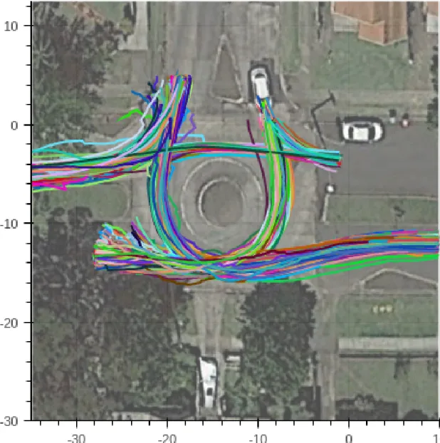
3.8 An overlay of 1000 of the recorded tracks at the intersection studied. 43 3.9 Heading profile of all tracks in the second dataset. . . 46
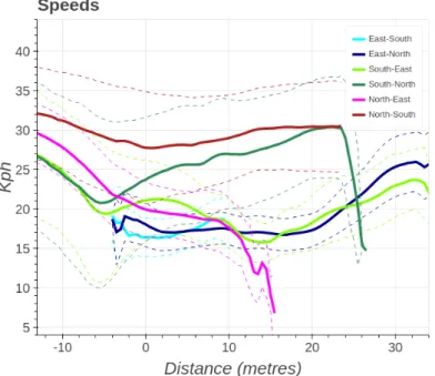
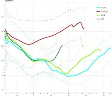
3.10 Speed profile of all tracks in the second dataset. . . 46
3.11 Satellite views of each of the five roundabouts in the dataset. . . 50
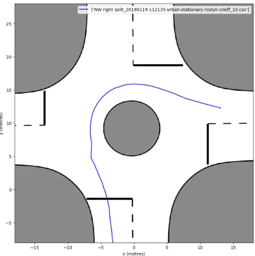
3.13 Heading profile of all vehicle tracks . . . 54 3.14 Speed profile of all vehicle tracks . . . 54 3.15 The tracked path of a single vehicle turning right at the intersection. 56 3.16 A sample of some of the corner cases in the dataset. . . 57 4.1 Diagram representing a RNN of length 5, that is given data for time t. 65 4.2 Diagram that depicts the individual layers of the RNN. . . 65 4.3 Accuracy of both the quadratic discriminant analysis (QDA) classifier
and the long short-term memory (LSTM) based RNN, when vehicles approach from the east. . . 67 4.4 Accuracy of both the QDA classifier and the LSTM based RNN, when
vehicles approach from the west. . . 68 4.5 Accuracy of both the QDA classifier and the LSTM based RNN, when
vehicles approach from the south. . . 68 4.6 A plot of the loss of a recurrent neural network during training that
overfits. . . 74 4.7 A plot of the loss of a recurrent neural network during training without
overfitting. . . 74 4.8 Diagram representing a RNN of example length 5, given data at time t. 75 4.9 Results of the classification model on drivers approaching from the east. 77 4.10 Results of the classification model on drivers approaching from the north. 78 4.11 Results of the classification model on drivers approaching from the south. 79 5.1 Predictions of the next 5 seconds after a vehicle has entered an
inter-section. . . 84 5.2 The path prediction problem in a graphical format. . . 85 5.3 Diagram representing a RNN with an input data sequence length of 5,
and an output sequence length of 5. . . 87 5.4 One dimensional Gaussian mixture model (GMM). . . 89 5.5 Two dimensional GMM. . . 91
5.6 The RNN-FL model at inference time 5.6a and training time 5.6b. . 97
5.8 The RNN-ZF model at inference time 5.8a and training time 5.8b. . 99 5.9 The output distribution of the RNN-FF algorithm. . . 101 5.10 The output distribution of the RNN-FF algorithm, for the same data
as seen in Figure 5.9. . . 102 5.11 Diagram presenting the stages of Multi-PAC . . . 104 5.12 An example of how two different manoeuvres may have the same error
metric. . . 106 5.13 An example of the modified Hausdorff distance (MHD) metric between
two lines. . . 107 5.14 Results from four different vehicles travelling in different directions. . 116 5.15 Results of a single vehicle turning right at several different distances
travelled past the reference line. . . 117 5.16 Several results of corner cases and failure cases. . . 120
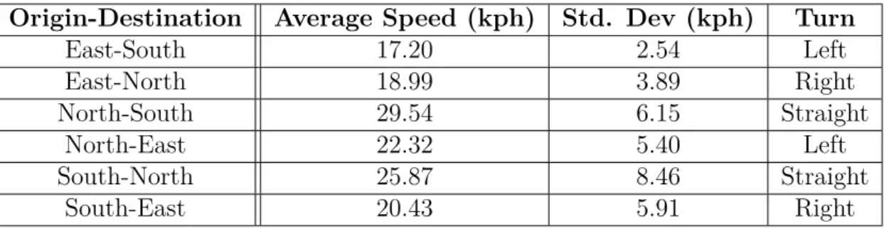
3.1 Summary of data collected at the roundabout, grouped by origin and
destination classes. . . 44
3.2 Table of the average speeds of each class, and their transition through the intersection . . . 44
3.3 Summary of Collected Data . . . 55
5.1 A table comparing the lengths of 95% of all the tracks turning in a particular direction. . . 94
5.2 Cumulative Results . . . 113
5.3 Results Grouped by Left Turning Vehicles . . . 113
5.4 Results Grouped by Vehicles Travelling Straight . . . 114
List of Symbols
t time-step, integer (units arbitrary) xt x co-ordinate of vehicle at time t, metres yt y co-ordinate of vehicle at time t, metres
θt heading of vehicle at time t relative to y axis, radians
vt velocity of vehicle at time t, kph
Vi entire sequence of data of vehicle i in the dataset
V The set of all Vi, the dataset
xt The input data at time t, typically [xt,yt, θt, vt]
Xt The set of all input data [xt−h...xt]
h the length of the observation sequence Xt
S The set of all training sequences, see equation 3.4
yt The ground truth data at time t
Yt The set of all ground truth data [yt+1...yt+p]
p the length of the prediction sequence Yt
ˆ
Yt a probability distribution estimate of Yt
y0t A single sample drawn from Yˆt
ci class (manoeuvre) of vehicle i
dt distance travelled to / from intersection line of vehicle at xt, metres
dj vector of all distances for vehicle j
ˆ
qt binary sequence length padding logit
L(x) loss function for neural network training α weight loss balancing hyperparameter β weight loss balancing hyperparameter
N() Gaussian (normal) distribution
M number of Gaussians in a mixture density network
π(j) Relative weighting of Gaussian j in a mixture density network µ(j)x x dimension mean of Gaussian j in a mixture density network
µ(j)y y dimension mean of Gaussian j in a mixture density network σ(j)
x x standard deviation of Gaussian j in a mixture density network σy(j) y standard deviation of Gaussian j in a mixture density network ρ(j) correlation coefficient of Gaussian j in a mixture density network τ thresholding value used in Multi-PAC
List of Acronyms
ACFR Australian Centre for Field Robotics
GPS global positioning system
IMU inertial measurement unit
GNSS global navigation satellite system
DSRC dedicated short range communication
GP Gaussian process
SAE Society of Automotive Engineers
RNN recurrent neural network
LSTM long short-term memory
MDN mixture density network
CV constant velocity
CTRV constant turn rate and velocity
CTRA constant turn rate and acceleration
DBSCAN density-based spatial clustering of applications with noise
MDN mixture density network
DNN deep neural network
QDA quadratic discriminant analysis
GMM Gaussian mixture model
Unsignalized: Without traffic lights
manoeuvre: executing a set of actions. Vehicle examples include lane changes and turning at intersections
multi-modal: [multiple modality] (of data) Having a disjoint probability i.e. there may be multiple solutions, but the average of any two solutions is not guaranteed to be another solution.
lidar: laser based ranging sensor
Introduction
In 2017, there were 1,225 deaths due to motor vehicle accidents in Australia [1]. This number has decreased significantly since its peak in 1970 of 3,798 [2], but it still too large. There has been significant effort through Australian Government mandates and campaigns to reduce this figure over the years, including mandatory seatbelts, random breath testing, and speed cameras [3]. In addition, there has been major advances in safety technology for consumer vehicles in the past 20 years including antilock brakes, traction control, crumple zones, rigid passenger cabins, multiple airbags as standard, and seatbelt pre-tensioners. These technology advances have allowed accidents that were fatal for passengers in a 1998 vehicle [4] to be reduced to negligible injuries in a 2015 vehicle [5]. The average age of a consumer vehicle on Australia’s roads is 9.8 years [6], but the average age of a consumer vehicle in a fatal accident is 13.1 years [7], showing that vehicle technology has made a major impact in Australia’s road toll. In addition to crash mitigation technology there are preventative vehicle technolo-gies which attempt to reduce or remove factors that lead to crash in the first place. These technologies, known as advanced driver assistance systems, include antilock brakes, adaptive cruise control, traction control, lane departure warnings, blind spot monitors, fatigue detection, and forward collision warning systems, to name a few. Even with advancements in road safety programs and vehicle technology the majority of accidents can be attributed to human error [8]. There is a movement to remove the
driver from the vehicle altogether, and so replace the human driver with a computer system, thus making the vehicle autonomous. Given the complexity of this task, the standards board Society of Automotive Engineers (SAE) International outlines five different levels of autonomy in SAE J3016 [9]. Level 0 involves no automation whatso-ever, and is completely driven by the human driver. Level 1 is driver assistance where one or more systems such as acceleration and braking is controlled by the computer, but all else is up to the human driver, including monitoring of other vehicles. Level 2 describes partial automation where the computer system has complete control in a very limited situation, such as lane keeping, and the human driver is expected to take over at a moment’s notice if requested. Level 3 describes partial autonomy, where the system is expected to monitor all surrounding vehicles on the road. Vehicles at level 3 are able to perform manoeuvres such as lane changes and traffic light navigation without human intervention. At this level, a take over by a human driver is still available upon request. Further levels describe a car that can fully navigate and drive a road without any human intervention, in either a limited road area (level 4) or all road areas (level 5). At level 5 the vehicle has no need for human controls such as a steering wheel or brake as it is expected to perform all operations by itself. For simplicity vehicles with any level of autonomy will be referred to as an ‘autonomous car’ in this thesis, and not just level 5 (fully autonomous) vehicles.
Given the average age of consumer vehicles on Australia’s roads is 9.8 years, there is going to be considerable overlap between when autonomous cars are first produced and when they are the only cars on the road. Optimistic predictions still have a majority of human driven vehicles over the next 30 years [10]. As such there is a need for vehicles to determine the intention and predict the path of other vehicles, so that they may interact safely. Technically speaking, methods for vehicle interaction are defined in the road rules. These rules define which vehicle must give way to others and defines the order in which vehicles should pass through an intersection. However, in practice these rules are not strictly adhered to, as human drivers have a more relaxed interpretation of these rules. Behaviours such as unsignalled lane changes, aggressive merges, or cutting corners are quite common on the road, and experienced human
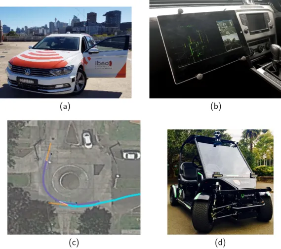
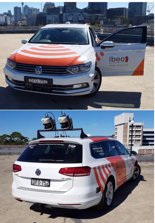
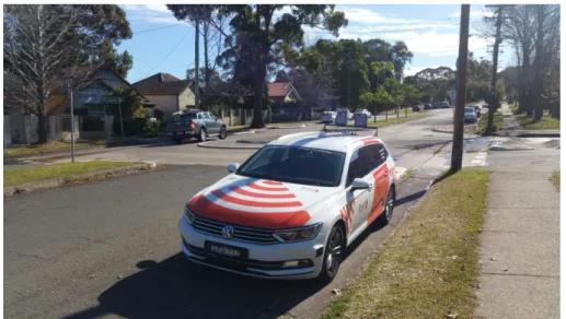
drivers have an intuition of what other vehicles are going to do. This thesis aims to capture this level of human intuition into a model that is usable by a computer, to aid in all levels of autonomous driving. The collection of intelligent vehicles used for autonomous car research at the Australian Centre for Field Robotics (ACFR) can be seen in Figure 1.1. The vehicle shown in Figure 1.1a is used for studying full speed traffic patterns, and data from this vehicle will be used extensively throughout this thesis. The real time tracking data can be seen in Figure 1.1b and a sample of some of the data used in this thesis can be seen in Figure 1.1c. The electric vehicle seen in Figure 1.1d is used for low speed fully autonomous testing.
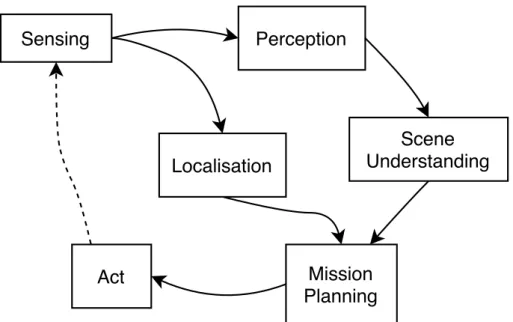
A simplified processing loop of an autonomous car is depicted in Figure 1.2. The process begins with sensing, as this is how the vehicle is able to gather data about the environment it is in. This describes which type of sensors are being used, such as camera, lidar or radar, and these sensors require an appropriate calibration. This raw sensor data is then passed to a perception system, which is able to identify objects and features in the scene, such as lane markings and other vehicles. Parallel to this is a localisation system, which is able to determine the position of the autonomous vehicle on a map. The perception data is then passed to a scene understanding module. This module is able to understand the surrounding scene and predict what the scene will look like in the near future based on context. This includes predictions such as: "A pedestrian is waiting at a crosswalk, therefore they are likely to cross the road." or "A vehicle is slowing down and moving to the outside of the lane as it approaches the intersection, how likely is it that this vehicle will turn into the side street?". This thesis will focus on scene understanding techniques, as it will present methods for vehicle intention and path prediction. The mission planner is then able to incorporate these predictions into a path planning algorithm that allows the autonomous vehicle to reach its intended destination while interacting with traffic. Finally, the mission planner sends commands to the vehicle’s actuators, namely the engine, brakes and steering wheel which allow the vehicle to drive.
Recent works in vehicle prediction have focused on vehicles in areas with significant infrastructure. This could be a multi-lane highway, or an intersection with traffic
(a) (b)
(c) (d)
Figure 1.1– The research vehicles used at the ACFR. Figure 1.1a shows the Lasercar, described in Section 3.4.1. The live tracking software can be seen in 1.1b. A sample of data collected for use in this thesis is shown in 1.1c with vehicles depicted as coloured rectangles, and their tracks shown as coloured lines. The second vehicle shown in Figure 1.1d is used in low speed autonomous testing.
signals and dedicated turning lanes. A significant proportion of accidents occur at intersections, of which 84% can be attributed to either recognition or decision error of a driver [11]. Whilst predicting driver intention at signalled intersections is currently an unsolved problem, there are considerable behaviour cues that exist because of the infrastructure. Vehicles in a turning lane at a set of traffic lights are near guaranteed to make the indicated turn, for instance. This thesis will focus on smaller, suburban intersections that do not have traffic signals and have only one lane. This makes prediction significantly more difficult as it cannot be based on traffic light phase, or
Sensing
Perception
Scene
Understanding
Localisation
Mission
Planning
Act
Figure 1.2– A simplified version of the processing loop that an autonomous car uses to sense, perceive and interact with its environment.
which lane the vehicle is in. These types of intersections are commonplace, and require significantly more driver interaction, as there are no traffic lights to dictate right of way or to demonstrate intent. As these intersections require human interaction, there is a tendency for road rules to not be strictly complied with, which can exacerbate assertive behaviour. Driving through these intersections is second nature for a skilled human driver, and is mostly based on an innate sense of intuition about the behaviour of other drivers. These intersections with such complex driver behaviours make an excellent challenge for any intelligent inference algorithm. The work of this thesis aims to capture this human intuition in a computer model for use in autonomous vehicle path planning and decision making. If a method can solve these highly dynamic scenes there is a high likelihood the method is transferable to more orderly scenes, such as highway lane keeping and lane change prediction.
There are a number of implementation constraints than need to be followed for the system to be practically deployed on an autonomous vehicle. These constraints are used through the thesis to ensure that the algorithms therein are able to be success-fully deployed. Firstly, the system must be fast enough to operate in real time, as
this is necessary for real time control. Secondly, the system may only use data that is available through on-board sensors and equipment. It must also not rely on data that exists in the future to run analysis about events in the present. Finally, the system should be generalisable, that is to say the solution should not be limited to one particular area.
Multi-Modality
This work focuses heavily on a multi-modality problem. In this thesis, the term ’multi-modality’ refers to multiple trajectory states of a vehicle. That is to say, when a vehicle traverses an intersection it typically may turn left, right or continue straight ahead. It cannot travel in the average of left and straight turns, as this would lead the vehicle to collide with the sidewalk. This is different to the typical use of multi-modal in similar works, which refers to different sensor modalities such as a combination of vision and lidar.
1.1
Contributions
The main contributions of this thesis are as follows:
• An analysis of current intention and path prediction techniques, as well as a study of the datasets available for this problem is presented in Chapter 2.
• From the analysis, a data driven approach was appropriate given the high di-mensionality of the problem. There are no publicly available datasets suitable, so a number of naturalistic datasets were collected for use in this thesis and are presented in Chapter 3. A description of the data capture vehicle is also pre-sented. At the time of writing, these datasets are the largest known collection of tracked vehicles passing through a specified set of unsignalised intersections. Overall, they equate to over 60 hours and over 23,000 tracks of vehicle data of
naturalistic human drivers traversing five different roundabout style intersec-tions in Sydney.
• Data wrangling and preprocessing techniques used in preparing the dataset for algorithm testing is presented in Chapter 3. In addition, a comprehensive analysis of this data is presented, such as manoeuvre frequencies, as well as speed and heading profiles.
• A novel application of RNNs for manoeuvre classification of the ego vehicle is provided. A method using LSTM based RNNs is presented in Chapter 4 for predicting the intent of drivers at intersections using manoeuvre classification.
• An extension of this technique for predicting the intention of external vehicles is provided in Chapter 4, which allows this system to be used with a lidar based object detection and tracking system.
• A real-time parametric model for producing vehicle path prediction with uncer-tainty is presented in Chapter 5. This model generates output that produces multi-modes that are discrete, each with uncertainty. Modifications to tradi-tional sequence-to-sequence loss functions are presented. The modes generated by the model are not hand labelled, but instead learned from the data. In ad-dition, proof of generalisability to similarly sized intersections is provided using the presented datasets.
Source code used for data wrangling, model training / testing, graph and table gen-eration can be found at: https://github.com/azyner/radip
The datasets used in this thesis have been made publicly available at:
http://its.acfr.usyd.edu.au/datasets/
1.2
Outline
The remainder of the thesis is outlined as follows. Chapter 2 presents a survey of similar work in driver intention prediction, and gives a background on Recurrent
Neural Networks. Chapter 3 describes why collecting a new dataset was necessary. It then introduces the datasets collected for this thesis, and presents some analytics about the collected data. Chapter 4 presents methods for driver intention prediction through the use of classification. Chapter 5 introduces a driver intention and path prediction model that is multi-modal and includes uncertainty. Chapter 6 summarises the thesis, presents a conclusion, and suggests future work.
1.3
Publications
The following works were published in the process of writing this thesis:
Alex Zyner, Stewart Worrall, and Eduardo Nebot. "Long short term memory for driver intent prediction." Intelligent Vehicles Symposium (IV), 2017 IEEE. IEEE, 2017.
Alex Zyner, Stewart Worrall, and Eduardo Nebot. "A Recurrent Neural Network Solution for Predicting Driver Intention at Unsignalized Intersections."IEEE Robotics and Automation Letters 3.3 (2018): 1759-1764.
Alex Zyner, Stewart Worrall, and Eduardo Nebot. "Naturalistic driver intention and path prediction using recurrent neural networks." Accepted, pending publication with
Transactions on Intelligent Transportation Systems, IEEE (2019).
Alex Zyner, Stewart Worrall, and Eduardo Nebot. "ACFR Five Roundabouts Dataset: Naturalistic Driving at Unsignalised Intersections." Accepted, pending publication with Intelligent Transportation Systems Magazine, IEEE (2019).
Background
2.1
Introduction
Driverless car research is nearly as old as passenger vehicles themselves. The first pub-lic demo of a "phantom motor car" was in 1926 by the Achen Motor company [12], which was a radio controlled vehicle driving public streets in Milwaukee, Wisconsin USA. Later in the 1950’s a lane guidance system based on detector circuits embedded in the street was developed by RCA labs [13]. This was adopted by General Motors for use in their prototype vehicle ‘Firebird’ in the 1960’s. This technology was never released for consumer vehicles, as it required major changes to infrastructure. Later in 1995, Carnegie Mellon University’s Navlab Project achieved semi-autonomous nav-igation, where the steering was computer controlled, and the accelerator and brakes human controlled for safety reasons [14]. In the same year, a team from Bundeswehr University Munich achieved an autonomous vehicle trip of 1,590 km of highway be-tween Munich and Copenhagen using a modified Mercedes-Benz S-Class, with a mean time between human takeover of 9 km [15]. Although there is still significant research to be done in the area of highway modelling, there are other driving scenarios that present very complex challenges worthy of study. Navigating intersections requires a driver to not only be aware of the infrastructure and lane markings, but also the driver must infer the intention and path of vehicles in the vicinity. Thus, a driver
needs to be aware of other vehicles that are not only driving in the same direction, but also oncoming traffic, and traffic on the intersecting roads. The next section will detail methods used for driver and vehicle prediction, which is a critical component for safe driving. The last section in this chapter, Section 2.3 presents background for Recurrent Neural Networks, a method that is prominent in the works presented in this thesis.
2.2
Related Works
Although the prediction of driver behaviour on the road has been widely studied, it is still an open problem. There are several approaches used in making predictions on driver behaviour. These areas are loosely grouped into physical based models, manoeuvre models, and path prediction models. These prediction techniques can be applied to the ego vehicle, that is the vehicle being driven, or externally observed vehicles, tracked using a variety of sensors.
Physics Based Models
Physics based models use kinematic or dynamic models to represent and predict vehicle movement. These approaches will represent the vehicle state with a physical based model, including parameters for speed, heading and acceleration, and then make predictions based on propagating this model forward in time. Popular approaches include a constant turn rate and velocity (CTRV) [16], filtering techniques applying Switching Kalman Filters [17], or Monte Carlo simulation [18] methods. These types of models are generally limited to very short term prediction (under one second) [19].
Manoeuvre Models
Manoeuvre based models make the assumption that the actions of the driver is limited to a set of manoeuvres. Given that there are only a finite set of destinations at an
intersection, these approaches will classify a vehicle by its destination, and sometimes by the origin-destination pair. Once the destination is predicted, the appropriate manoeuvre (e.g. turn left, turn right, change lanes) can de determined. This allows the rest of the vehicle’s motion to be predicted, as it should match the manoeuvre. A variety of algorithms have been tested for classifying driver behaviour into ma-noeuvres, including multi-layer perceptrons [20], support vector machines [21] [22], relevance vector machines [23], conditional random fields [24], Bayesian networks [25] [26] [27], and hidden Markov models [28] [29] [30]. The use of support vector ma-chines [31] and Bayesian regression [32] has also been explored for large (>20 metres in diameter) roundabouts. Most of the existing works generally rely on tracking data taken from the ego vehicle. Other works focus on adding sensors to the internal cabin of the vehicle, such as a camera pointed at the driver. This allows analysis of the driver’s attention, and use of that as input to a prediction model. Roth et al. [33] use this information as the input to a dynamic Bayesian network to predict stopping behaviour, while Jain et al. [34] include head pose as input to an RNN for manoeuvre prediction. Other internal sensors are also used, such as hand and brake pedal cameras [24]. However, adding these sensors to consumer vehicles is costly and impractical.
The first half of Chapter 4 explores the feasibility of using LSTM based RNNs for manoeuvre prediction at a suburban, single lane unsignalized intersection. It focuses on analysing multiple, consecutive time steps of data and classifies a vehicle by its predicted destination. This allows for analysis of how early an accurate prediction can be made. The solution runs in real time, requiring about 60 milliseconds of compute time. Only vehicle state information is used in the prediction, specifically: GPS location, heading, and speed. These works rely on vehicles being outfitted with a dedicated short range communication radio, so that the vehicles may then broadcast the driver’s intent to neighbouring vehicles. As there will be vehicles without this type of technology on the road for the foreseeable future, it is necessary for an intelligent vehicle to infer intent about neighbouring cars. This data could be collected by a smart intersection which uses overhead cameras or overhead lidars [35]. An LSTM
based solution is presented by Phillips et al. [36] that focuses on large, multi lane intersections in the US., using features such as speed, which lane the car is in, and information about the surrounding six vehicles.
An intelligent vehicle will not be able to solely rely on smart infrastructure to gather information as not all intersections will be equipped with such features. So the system must be able to infer intent of surrounding vehicles using on-board sensors alone. Muffert et al. [37] present a stixel based stereo vision solution at a large urban roundabout, using a time-to-collision based metric. A similar method is used by Barth et al. [38] focusing on a turn-across-lane scenario using both real and synthetic data. Using the KITTI dataset, Khosroshahi et al. [39] present an LSTM based method to classify tracks through a signalised intersection, as recorded by lidar data. The data used is very limited as only 49 tracks were used. This method summarises the track into a collection of features at even intervals, and the entire collection is fed into the model at once. This includes data for the endpoint, which prevents this model from being predictive.
There is little focus on less structured, single lane, unsignalized scenes. The latter half of Chapter 4 details a data-driven method for determining driver intention at one such intersection, using data collected with a lidar based tracking system.
Path Prediction
Predicting the manoeuvre, and therefore the destination of a vehicle is helpful, but it would be far more useful to predict the entire trajectory of the vehicle. Having an estimate of where surrounding vehicles are going to go allows an autonomous vehicle to plan around those vehicles. Path prediction models attempt to produce a future trajectory of a vehicle given some data on the vehicle’s past. Often, physical based kinematic or dynamic models are used in conjunction with switching Kalman filters [17], Monte Carlo simulations [18], or variational Gaussian mixture models [40]. These methods will output a single prediction proposal, and give a measure of uncertainty. A manoeuvre recognition system can be combined with a Gaussian process based
path predictor to allow multi-modal prediction [41]. More recently, there has been a focus on data driven approaches for this task, as there has been recent advances in hardware designed for deep learning.
A commonly used dataset for this work is the NGSIM highway datasets, US-101 and I-80 [42]. This dataset was collected in 2005 using multiple overhead cameras observing sections of highway. This data was taken over three sections of 15 minutes each and contains trajectories of roughly 5000 vehicles. Visual tracking techniques were used to extract vehicles trajectories from the image data at a rate of 10Hz. Given the nature of tracking vehicles from a distant camera, the data suffers from considerable tracking noise [43], and even with aggressive filtering and correction techniques, significant problems still exist, such as multiple collisions [44] that do not exist in the real-world scene. We overcome these limitations with a modern data collection vehicle, as later described in Section 3.4.
Using the NGSIM dataset, Morton et al. [45] use an LSTM based RNN to predict the acceleration profile of drivers over a ten second window. Using the acceleration profiles to determine velocity and therefore position is useful, but it does not include any other manoeuvres, such as lane changes. They extend their model using gener-ative adversarial networks [46] to produce full trajectories. To allow this model to incorporate the movement of surrounding vehicles, the authors simulate lidar returns derived from vehicles in the NGSIM dataset. The lidar is approximated by a single beam spaced out at 20 even intervals, and it is assumed that this beam is perfectly horizontal, centred at the vehicle centre.
Vehicles paths on highways can also be predicted using an occupancy grid. By using an embedding layer before the RNN, Kim et al. [47] encoded vehicle positions using a one-hot map. To predict the vehicle’s locations at different time horizons (0.5 seconds, 1 second, 2 seconds), an entirely new network is trained for each horizon. The data used in these experiments is captured using Delphi long range radars, and consists of 1325 vehicle tracks. The work is extended by Park et al. [48] to use a encoder-decoder RNN, allowing for a single network to produce the target vehicle location prediction for all time horizons. This particular network configuration allows beam search [49]
to be used, which increases the output search space of the network, which in turn aides model accuracy. The occupancy grid encoding configuration does not allow for the similarity of neighbouring cells to be properly represented, and so this must be learned by the network.
The work by Deo et al. [50] uses a variational Gaussian mixture model combined with a hidden Markov model. This method generates a prediction of the manoeuvre the observed vehicle will perform, and then uses the variational Gaussian mixture model to produce a prediction of the path the vehicle will take, with uncertainty. This method is validated on a dataset collected by the authors using a vision based system. A mere 48 tracks are used for training sequences, which are then inflated with data augmentation techniques. Four tracks are used for the evaluation dataset, and are human annotated.
Multi-modal Path Prediction
The future path of a vehicle can be described as a multi-modal problem. That is to say, there are multiple modes (destinations) a vehicle can take an an intersection, but the combination of these modes is not guaranteed to be another valid solution. As such, a single path with uncertainty is inappropriate, so multiple possible predictions must be proposed. Recently there has been an upsurge in the use of recurrent neural networks used for trajectory prediction. These data-driven models build off of the work from Alex Graves [51] that was produced for handwriting generation. This model is a sequence-to-sequence model that includes a mixture density network (MDN) output layer, which allows the model to produce a probability distribution. The probability distribution is represented by a sum of weighted Gaussians, usually on the order of six to twenty. The output distribution can then be multi-modal i.e. there are multiple distinct peaks in the output distribution. This in turn, allows for multi-modal trajectory prediction, as there may be more than one possible path for a vehicle to take but the combination (by averaging or otherwise) of multiple paths does not necessarily produce a valid new path. Multi-modality and mixture density networks will be discussed in length in Section 5.5. The original method presented
by Graves trained the model against the next time step during model training. To produce data at the next time step, a single sample is taken and fed as the ‘ground truth’ for the next sample, and so on in a feed-forward fashion. Doing so collapses the multi-modality of the output distribution and the model only produces a single path. The output predicted in this model is the change in position, which needs to be added to the previous data to get the next co-ordinate in the path.
A modification of this technique that incorporates the movement of surrounding agents, Social-LSTM, was produced by Alahi et al. [52]. This is the LSTM-MDN technique applied to pedestrian movement, with an added social convolutional layer that allows agents to determine intent of other agents. However, this solution only produces a single mode, as instead of using a mixture density network the authors chose to use a single bi-variate normal distribution. This is equivalent to a MDN with a single Gaussian.
It is significantly more useful to not just predict a single trajectory with uncertainty, but to predict all the possible manoeuvres that an agent may take, and assign each a probability. This allows the mission planner to consider all possible trajectories, to make a better informed decision. Deo et al. [53] improve on their previous work by using this Social-LSTM scheme combined with a manoeuvre classifier. This classifier is trained to predict manoeuvres in the set of [lane change left, lane change right, keep lane], combined with [keep speed, reduce speed]. By training one network per manoeuvre class, they are able to produce a system that produces one trajectory per possible manoeuvre, and are ranked by the classifier.
Conditional variational autoencoders for trajectory prediction are another technique that have been adopted from simulated handwriting. The work of Google Sketch-RNN [54] adds the MDN layer to a variational autoencoder to reproduce drawings. A variational autoencoder is a type of network that is able to learn to reproduce patterns. The variational input allows a level of stochasticity to be introduced, which in turn allows for different drawings to be produced. A conditional variational autoencoder [55] allows a variational autoencoder to be conditioned on an input. Using this model, the trajectory of an agent can be predicted by conditioning on the agent’s
path. This technique has been recently adopted for use in vehicle path prediction and vehicle interaction modelling. Schmerling et al. [56] use this model to plan a vehicle’s behaviour based on sample data taken from a human-in-the-loop simulator. By sampling multiple times from the conditional variational autoencoder, a collection of trajectories can be produced, however these are not ranked. The mean and variance of this population of trajectories is used to compute uncertainty. A modification of conditional variational autoencoders to rank these outputs is produced by Lee et al. [57]. Their work ‘DESIRE’ is tested on both a subsection of the KITTI dataset and the Stanford Drone dataset, demonstrating the transferability of these techniques between vehicle and pedestrian prediction, given sufficient data. Although their prediction output appears to be multi-modal, it is unclear how many times the network needs to be sampled from to expose all the modes in the prediction. While these samples may be ranked, uncertainty of each prediction is not given.
Chapter 5 will present a method for predicting the path a vehicle. The method is able to produce multiple modalities from a single run of the network, so it is able to be run in real time. Each of the modalities has uncertainty, and these paths are ranked according to their probability. The number of modalities is not hand crafted, so there may be vehicles that only have two possible modes (such as go straight, turn right) given their speed during the intersection approach. This method is validated at a suburban roundabout, a kind of unsignalised intersection. Predicting vehicles at an unsignalised intersection introduces significant complexity, as is not as highly structured as a highway environment, and there are no traffic signals to dictate which vehicles must give way.
Deep networks have also been shown to be useful in vehicle path planning. However, as these methods involve interacting with the scene, gathering data and validating the system is extremely difficult. These works typically will use full simulators [58] [59], human in the loop simulators [56], a tightly controlled test course, or some combination of all [60]. Validating the use of simulators is difficult when modelling real-world scenarios that involve risk as there is no equivalent risk present in the simulator [61]. Simulators which are closed source are even harder to validate, as often
details of how the synthetic data is generated are omitted. Without this information there is no way to tell if the scenarios generated by the simulator are realistic, and so it does not give any real-world performance indication of the algorithm under test. Given that the vehicle prediction problem is still largely unsolved, and the difficulty of validating a decision making system, these works are outside the scope of the thesis.
Prediction Scenarios
The prediction of driver behaviours on highways have received significant attention during the past few years. This is not the case for intersections, even though these areas account for a large proportion of accidents — around 40% [11]. There are a few publicly available datasets that cover these scenarios that are widely used. Nev-ertheless, they all have fundamental drawbacks when being considered for testing algorithms deployed on an autonomous vehicle. One such dataset is the Ko-PER project, but this is taken from an overhead perspective to simulate smart infrastruc-ture [35]. Overhead sensors do not capinfrastruc-ture the sort of perspective issues on-board sensors would, and this dataset does not include tracking information, only sensor in-formation. As previously mentioned, NGSIM datasets Lankershim and Peachtree are also often used, and this is data collected from an overhead camera passed through a visual tracking algorithm. The NGSIM dataset contains significant tracking errors [44], and is only 45 minutes of data per scenario. For data that is taken onboard a vehicle, it is common to take data annotations from KITTI and use that in lieu of an actual tracking algorithm, further abstracting the solution away from a practicable pipeline [39]. The use of human annotations assumes that a tracking system that is as good as a human (with infinite labelling time) is available, which is generally not the case. Most of these datasets are of a structured intersections with easily visible lane markings and traffic signals, and there is little focus on unstructured, unsignalised settings. A more in depth survey of recent datasets will be presented in Section 3.2.
2.3
Recurrent Neural Network Background
The works in this thesis make use of recurrent neural networks (RNNs). To under-stand RNNs, first under-standard neural networks need to be described. This section will describe simple neural networks, deep neural networks, recurrent neural networks, and touch on batch optimisation and hyper-parameter selection. Neural networks are a data driven technique, and in recent years have become popular, in part due to an increase in available data, as well as optimisations in computer hardware. These networks have been used to solve a plethora of problems, such as image classifica-tion, text generation and object detection. The fundamental building block of a deep network is a single perceptron, which is explained in the next section.
2.3.1
Simple Neural Networks
Figure 2.1– A single perceptron, with three inputs. [62].
A neural network consists of several artificial neurons (aka perceptrons) connected as nodes in a graph. Each of these nodes will have an output activation a according to the function: a=f( N X i=1 Wixi+b) (2.1)
where N is the number of inputs,W is a vector of weights, andbof biases, which are learned parameters of the model. This is then wrapped in an activation function f to increase the complexity of the model as it adds non-linearity. Common examples of the activation function include tanh, sigmoid, or Rectified Linear Unit. However, a single neuron is not particularly useful as it is too simplistic to learn higher level
Figure 2.2– A basic multi-layer perceptron. Here many neurons are combined to form layers, and many layers are combined to form the final network. Image sourced from [62].
functionality. Instead, these neurons are often bundled together in layers, and these layers are stacked to form a multi layer perceptron, seen in Figure 2.1. A multi layer perceptron is a basic form of deep neural network (DNN) where each layer is fully dense — that is all nodes from one layer are connected to every node of the previous layer. There are three types of layers that are typically addressed, these are the input layer, the hidden layer, and the output layer. The input and output layers are self explanatory, and the hidden layers are all the layers in the middle that do not get directly exposed to the input or output data. A simple multi-layer perceptron can be seen in Figure 2.2. DNNs are trained to be used as large non-linear functions, and typically are trained to solve either regression or classification problems. Regression problems are where the model is attempting to produce a single output as a floating point number, an example of which is estimating the price of a certain share given historical data. Classification problems are where the model assigns a single label to the input data from a given set of labels, an example of which is sorting skittles by their colour.
These networks are trained through an optimisation process known as back-propagation. A DNN is first initialised with random weights, and inference is run on the network by inputting a training sample. This will then propagate data forward through the
nodes until a final solution is produced. This solution will be compared to the ground truth data, which is the correct label for this input data. This produces the error of the network, which is generated by some loss function — typically cross entropy loss for a categorisation network. By differentiating through each layer of the network, a gradient can be found, allowing the optimiser to update the weights of the network for this training example. This is repeated for every sample in the training set. As with all optimisers, this is done with a very small step size. If the step size is very large, weights can inflate and the model will not converge. To speed up the training process, multiple samples can be used as training data at once, in a process called batching where the update weights are summed.
Another aspect to DNNs are hyper-parameters. There are many parameters used in both the model definition and the training, and values for these parameters need to be found. Some of these parameters include: the number and type of layers, the width of each layer, the learning rate, the optimiser, and the batch size. While some parameters have little influence to the final result such as the batch size, others need to be tuned. This is mostly done through a grid search, where each value is tried in turn, and the final performance of each network compared. Bayesian optimisers exist to optimise the hyper-parameters, but in practice these often under-perform when compared to an expert grid-search.
Other types of layers found in DNNs include the convolutional layer, which allows the network to learn specific gradient patterns. Some layer types are not learnt, such as drop-out. This is a type of over-fitting prevention technique, where during training, a random sample of neurons are set to zero, as to have no activation. This prevents the network from only looking for a specific feature, but instead enforces the solution to be a combination of some features, by deleting some features randomly.
2.3.2
Recurrent Neural Network Layouts
Standard neural networks will have one input, and one output. Instead, a recurrent neural network can have multiple inputs, and multiple outputs by re-running the
A
h
tx
t=
A
h
0x
0A
h
1x
1A
h
2x
2A
h
tx
t...
Figure 2.3– A basic recurrent neural network
network on the new data, while maintaining some internal data between the two network runs. The weights of the neurons remain the same, but the activations differ because the input data differs, and there is state information that is retained. This can be thought of as having a ‘flip-flop’ inside a neural network — these networks can store and act on data that happened an arbitrary length of time ago. In this way, a single RNN layer has two inputs and two outputs, with one set in data and the other in ‘time’. The use of the word ‘time’ and ‘time-steps’ is loose, in this context it refers to a single recurrence of the network, and describes traversing any sequence: be that words in a sentence, instructions in a program, or frames in a video, for example. An ‘unrolling’ of an RNN in time can be seen in Figure 2.3. Here the network has one input xt and one output ht per time-step. The weights of the recurrent network A remain the same across time steps, but the activations differ as the internal memory changes over time, and the input differs over time.
There are many layouts an RNN can have, which can be seen in Figure 2.4. The first one is the most basic, and it represents a typical DNN, with one input, and one output. The next type depicted is a one-to-many network, where the output is a sequence, and the input is a single data sample. An example of this is an image caption generator where a single image is served as input to the network, and the network produces a sentence — a sequence of words. This sentence has no fixed length, the network runs until the ‘end of line’ character is produced by the network.
one to one one to many many to one many to many many to many
Figure 2.4– Several different layouts of RNNs
The third network shown is a many-to-one configuration. Chapter 4 explores this type extensively by categorising the track of a moving vehicle. The next two types of RNN are both many-to-many. The first is where a whole sequence is input before a sequence is output, which is the format of the language translator presented in [63]. The final example is where there is an output for every input during the sequence, an example of which is video classification that may change as the video progresses.
2.3.3
Recurrent Neural Network Cells
Using standard dense layers in a recurrent configuration does not work very well. This problem is similar to why very deep networks fail, there is an issue known as the vanishing gradient problem. There are many layers that back-propagation needs to update and these gradients diminish for every layer it passes through, resulting in that they converge to zero rather quickly. To solve this problem a new network cell type needs to be used, and the most common one is the LSTM module.
There are four components to an LSTM [64], the input gate it, the output gate ot, the forget gate ft, and the cell ct. These can be seen in Figure 2.5. The input gate controls whether input data is stored in the cell. The output gate controls if the data in the cell is passed to the LSTM output ht. By retaining information in the cell, activations can be maintained between time-steps, and are influenced by the input gate and the forget gate. This allows the LSTM module to hold information for an arbitrary amount of time, as the derivation of the cell contents is constant, which allows the gradients to propagate through every layer in the network. This can be
Figure 2.5– A single cell of a long short term memory module. [51]
thought of as an electrical ‘flip-flop’ in a neural network. Mathematically they are also similar to skip connections used in very deep networks.
There are many other types of cells that also solve the vanishing gradient problem such as the gated recurrent unit [65], or modified LSTMs: such as the hyper-LSTM [66], and batch normalised LSTM [67]. In practice, the type of recurrent module used becomes another hyper-parameter for the system.
Datasets: Collection, Analytics and
Preprocessing
3.1
Introduction
Datasets are critical for the evaluation of a particular method. Significant care must be taken to ensure the data collected allows for proper representation of the problem to be solved. Only after verifying that the data properly encapsulates the problem can the method under test be assessed for suitability of deployment. To properly represent the problem, the data must be collected as close to the scenario where the algorithm is deployed as possible.
In regards to studying traffic patterns relevant for autonomous vehicles, a good dataset is taken in situ — it is taken on a real vehicle, on public streets. This is because data collected this way best matches the perspective of the use-case. If the algorithm is to be used with on-board vehicle sensors, there is no guarantee that this algorithm will perform similarly if the dataset used for algorithm training and validation was collected using overhead sensors. Although we may expect the use of intelligent infrastructure to supply data to individual vehicles in the near future, there will still be a majority of intersections without any such system. Ideally collected data
is completely naturalistic, the driver should be comfortable in the vehicle such that they drive the way they normally do. Furthermore, data that is representative of the problem should be collected publicly, where the public are driving their own vehicles, and are not aware of the dataset being collected. Only then can the dataset capture nuances in driver behaviour, such as negligent driving, speeding, or assertiveness. Corner cases such as these can be more commonplace than one would expect, and all sorts of driver behaviours must be accounted for if autonomous driving is to be achieved.
Given the difficulty of collecting data, some works have instead chosen to use a sim-ulator to create synthetic data of the scenario. This can range from a simple custom written simulator, or a more advanced off the shelf product like IPG CarMaker [68]. Methods that use a custom written simulator usually provide little detail in how the simulator was written, which makes it difficult to understand how well the model per-forms. Works that use synthetic data usually assume some level of perfect knowledge from the scene, that is usually impossible to acquire in real-world scenarios. One such example is the assumption of perfect localisation, where the ego vehicle’s loca-tion is not influenced by GPS inaccuracies, which are quite common in urban areas due to the urban canyon effect [69]. Another common assumption is perfect tracking information, where there is no noise in the location estimate of other vehicles and there is perfect re-association when a target is lost due to occlusion. A third common oversight is assuming a perfect perspective of all the agents in the scene, but in reality it is impossible to observe everyone in a scene from a moving vehicle, as there are occlusions from other vehicles.
There is no guarantee a method that performs well on simulated data without incor-perating these types of errors will perform well in a real-world scenario. Simulators also do not properly capture the driving style of humans, there is no guarantee that the way the simulator drives the vehicle is similar to how a human would drive one. Speeding, negligent driving, failure to yield are all common on the road today, and these corner cases are rarely represented in a simulator. Some works use a driving simulator to capture the actions of human drivers [56]. Validating the use of
human-in-the-loop simulators is difficult when modelling real-world scenarios that involve risk as there is no equivalent risk present in the simulator [61].
The dataset must also be sufficiently large to properly analyse the performance of the method under test. It is necessary to split this data into training and test sets such that the dataset used for algorithm validation is completely separate from the dataset used in training. If the dataset contains very few samples (less than 150) and is split in a 4:1 ratio for training and test, this leaves only a handful of samples in the test set, which diminishes the precision of the reported algorithm performance. After presenting a review of driving datasets this chapter will outline three datasets that are used in this thesis. The first, the ‘Naturalistic Intersection Driving Dataset’ was a collection of 198 traversals of an unmarked T-intersection in urban Sydney collected by Bender et al. [70]. The next two were collected by the author using a vehicle fitted with an Ibeo lidar detection and tracking system. The second dataset is of 8,292 vehicles traversing a T-style single lane roundabout in suburban Sydney. This dataset contains approximately 20 hours of data collected over 2 days and con-sists of naturalistic trajectories of public vehicles passing by during this time. This incorperates data collected at different times of day and very different traffic condi-tions. The third dataset expands this collection considerably by adding four more intersections, all of which have four exits. This leads to a collection of over 23,000 vehicle tracks at unsignalized intersections taken over 60+ hours.
Roundabouts are used as a test case for the works in this thesis. These small unsignal-ized intersections involve highly variable manoeuvres and are significantly more com-plex than the vehicle manoeuvres that occur on highways and in other structured environments. A dataset sufficient to study these aspects was not publicly available, and so collection of data was essential for this thesis.
3.2
Related Works
Driver behaviour at intersections has been a widely researched topic for some time. There are many available datasets that focus on intersections in several countries. One such popular dataset is the Next-Generation Simulation (NGSIM) [42] dataset that includes 45 minutes of tracking data of two lane highways, and two multi-lane intersections in the United States. The dataset includes the position and speed of vehicles as computed by a visual tracker from several overhead cameras. Whilst this data may be commonly used, the quality of tracking information is poor. This dataset contains as many as 747 collisions [44] when considering the raw data which did not occur in real life. The scope of NGSIM is also quite narrow as it only contains 45 minutes of data per scene and focuses on large road infrastructure in the United States.
Other datasets that focus on intersections exist, such as The MIT Trajectory Dataset [71], The MIT Traffic Dataset [72], the Computer Vision and Robotics Research Tra-jectory Analysis dataset [73], the Queen Mary University of London Junction Dataset [74], the Ko-Per project [35], the Karsruhe Institute of Technology intersection dataset [75], the Urban Tracker dataset [76], and the Idiap traffic junction dataset [77]. All of these datasets contain colour imagery from overhead traffic cameras, and are often of a low resolution (480x720, or even lower 288x360). Some datasets contain multiple overhead views and lidar scans. Ground truth annotations of selected sections of the data is available, but often not for the whole dataset. Moreover these datasets only contain raw sensor data. The output of a tracking solution is not available. The user must implement a tracker if trajectory data is desired. With the exception of the MIT Trajectory Dataset which is of a carpark, all other datasets focus on multi-lane intersections with traffic signals.
Instead of using overhead sensors, there is a recent uptake of published datasets of data taken from sensors onboard vehicles. These vehicles are then driven many hours across a wide variety of scenery and locations. A widely used dataset is The KITTI Vision Benchmark suite [78] — which has been extended to include other
sensor modalities such as a 64 beam Velodyne lidar, stereo cameras, GPS and an inertial measurement unit (IMU). Similar datasets that focus on driving sensor-laden vehicles include the Udacity dataset [79], comma.ai’s dataset [80] and Brain4Car’s dataset [81]. All of these are of vehicles driving through different cities with KITTI focusing on European cities, while the other are mainly of the San Francisco bay area. They cover a wide variety of different roads and traffic scenes, but do not stay in one place. This makes it difficult to study specific intersections in these datasets on a case-by-case basis, as there is very little data at each intersection. To study behaviour of nearby vehicles at an intersection it is possible to isolate different sections of these datasets. This allows analysis of vehicle trajectory and motion patterns at different intersections. However, each of those intersections has to be labelled and the ego recording vehicle does not stay at each intersection for a considerable amount of time. This makes the return on annotation investment very low. In addition these datasets do not have tracking data, only raw sensor data so a tracker must be implemented. More commonly, the subset of the dataset with ground truth annotations is used in lieu of a real-time tracker. Other large datasets exist, such as Apolloscape [82], CityScapes [83], and the more recent UC Berkeley BDD100k [84], but these only contain camera information, and any depth information is limited to that collected from a stereo camera.
There are no available datasets that contain large amounts of data of naturalistic vehicles at an intersection from the perspective of an autonomous vehicle. Collect-ing data at ground level instead of overhead introduces occlusion errors which can be a major source of tracking errors. The available datasets for intersections focus on areas that have considerable infrastructure, such as multi-lane roads, highways and traffic lights. Smaller, unsignalised intersections that are common in suburban neighbourhoods are not often studied. These intersections have no strict ordering of vehicles as there are no traffic signals, so there is considerable negotiation between vehicles at these locations. Often drivers are assertive at these intersections, and can fail to give way to other vehicles when necessary in order to get ahead of others at the intersection. Drivers may slow down and move to the centre when turning across
other lanes — a right turn in Australia. Others may unnecessarily move to the centre of the road before turning left as if they were towing an invisible trailer. To study behaviours such as these it is necessary to collect a large amount of naturalistic data focused on unsignalised, single lane intersections.
3.3
Dataset 1 - Naturalistic Intersection Ego-Motion
Driving
The first dataset used in this thesis considers the ego vehicle information and was collected by Bender et al. [70]. A brief description is included for completeness as it is used in Section 4.2.
This dataset, known as the Naturalistic Intersection Driving Dataset, consists of 198 paths travelled through an unmarked T shaped intersection, as driven by three different drivers. A satellite view of this intersection can be seen in Figure 3.1. This set consists of 6 possible manoeuvres. From each of the three approaches, there are two different turns a driver may take, thus creating six different manoeuvres. Each driver was instructed to perform each manoeuvre 10 times. A driver will behave differently depending on their intended manoeuvre — this can manifest in a different trajectory, velocity profile, or changes in heading. The aim of this dataset is to capture the potentially subtle cues based on the way a driver approaches an intersection. This allows a model to analyse a combination of kinematic features and location context to model the intended destination, as executed by a manoeuvre.
Each manoeuvre a driver can take has different characteristics leading up to the intersection. For instance, a driver turning across traffic will slow down and move to the centre of the intersection. The driver may have to come to a complete stop to give way to other traffic. A driver making a close turn will generally move to the outside of the road and slow down in preparation for the turn. A driver continuing straight will most likely do none of these things, and maintain speed and heading. These subtle differences in driving behaviour are the features that are exploited in
this classification algorithm, so that an intelligent vehicle can predict the intentions of its driver, and potentially transmit that to other vehicles connected via dedicated short range communication (DSRC).
3.3.1
Data Preparation
The position data for the vehicle was recorded at 10 Hertz by a global navigation satell