Large-Scale Analysis of Protein-Ligand Binding Sites using the Binding MOAD Database.

(1)

Large-Scale Analysis of Protein-Ligand Binding Sites Using

the Binding MOAD Database

by

Nickolay Khazanov

A dissertation submitted in partial fulfillment of the requirements for the degree of

Doctor of Philosophy (Bioinformatics) in The University of Michigan

2012

Doctoral Committee:

Professor Heather A. Carlson, Chair Professor Brian D. Athey

Professor Daniel M. Burns Jr. Associate Professor Yang Zhang

(2)

(3)

ACKNOWLEDGEMENTS

I would like to acknowledge the long term confidence and support of Dr. Heather Carlson. Her passion, dedication, and attention to detail have set the standard for my current and future scientific endeavors. I am proud to have been part of a team that was dedicated to exciting and quality research, and I will always be honored to have been a HACer. I humbly thank my dissertation committee and the Bioinformatics program directors for their time, insightful advice, and saintly patience and support all along my winding road through the program.

I would like to thank the current and past members of the Carlson lab for making my work possible. Binding MOAD would not be the great scientific tool it is today if it wasn’t for tremendous efforts of Richard Smith and Mark Benson, my brothers-in-arms in the ongoing fight for more binding constants. The wonderfully-elegant HwRMSD project would not have been possible without Kelly Ganamet and timely help from Daniel Quang. I acknowledge Jim Dunbar for his sage advice, and many hours of helpful and engaging scientific discussion. Thank you to Jerome Quintero, Katrina Lexa, Anna Bowman, Michael Lerner, and Man-Un (Peter) Ung for their tremendous friendship and wiling participation in the many therapeutic lunch breaks and coffee-runs.

Many projects in this thesis would not have been possible without the tremendous work done by the open-source scientific community. I wish to acknowledge the MySQL consortium for their constant improvement of the MySQL database, the Python community for many great libraries like NumPy and Biopython, the Django Project for their wonderful web framework, Ethan Merritt and Jay Painter for their mmLib library, and Warren DeLano for the outstanding PyMol application. Thanks go out to John Beaver, Brandon Dimcheff and Peter Dresslar at Torrey Path LLC, whose BUDA

(4)

application has saved me countless hours of laborious effort that can accompany the annual Binding MOAD update process.

I extend enormous thanks to my family for their patience and long-term support in my pursuit of this degree. Their thoughts of encouragement were with me even though they were many miles away. They never lost faith in my potential, even when my own confidence faltered. Thank you for all your kind words of support, the many phone calls and your patience during the long periods between my visits home.

Last, but definitely not least, I would like to acknowledge my friends, both in Ann Arbor, and in Edison. You have all provided me with limitless inspiration, motivation, and general good vibes. I will not forget the great memories made during my time at Michigan. The biggest thank you goes out to Yuri Ikeda, who has directly (as the Bioinformatics student services coordinator) and indirectly (as a personal friend and companion) sacrificed much of her time and energy to make this work possible. Her bright smiles of support in times of success, and her firm hand-to-the-forehead smacks in times of un-warranted despair, have been major motivating factors in the completion of this work.

The work in this thesis was supported by a Training Grant from the National Institutes of Health (GM070449-01A1) and NSF Career Award for HAC (MCB

(5)

LIST OF FIGURES

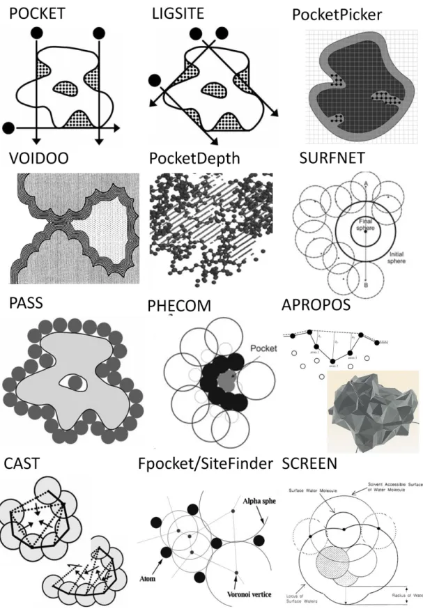
Figure I-1: Illustration of several methods utilizing protein-structure geometry for binding-site identification. Each illustration is taken from the publication describing the respective algorithm. ... 11

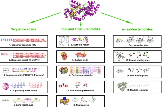
Figure I-2: Schematic of different methods used by the ProFunc server to predict protein functional sites and infer protein function in general. The right-most column lists 3D template methods used to match potential cavities to existing PDB entries. Figure taken from Laskowski et al. [69] ... 21

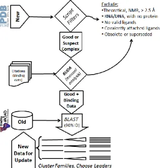
Figure II-1: Annual growth of the PDB. Figure from rscb.org ... 35 Figure II-2: Annual update of the Binding MOAD database and description of the individual steps. ... 36

Figure II-3: Literature citation analysis tool (BUDA). Inset shows text highlighting that identified sentences likely to contain binding data. Data and ligand annotations are recorded in allocated fields and saved for eventual export to Binding MOAD. ... 39

Figure II-4: Simplified entity relation diagram for the Binding MOAD relational database, illustrating the relationship between A) the protein, ligand, and binding-data annotations in the existing schema and B) the structure’s residue, atom, protein-ligand interaction, and residue-count data in the extended schema. There is a one-to-many relationship between the central table in A (ligandsuperrelationejb) and central table in B (moabs_bindingsite). Some tables and fields omitted for clarity. ... 43

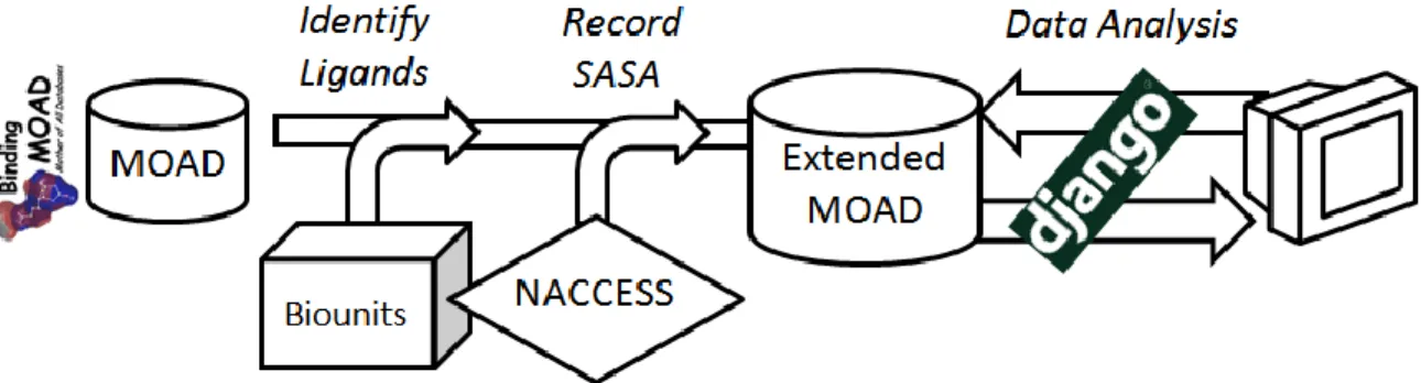
Figure II-5: Implementation of the extended Binding MOAD database. Scripts are used to load the extended database. A Django-powered front end implements data analysis and display functions. ... 46

Figure II-6: Example of a query for calculating residue propensities for a set of binding sites (in this case all valid binding sites with side-chain contact residues in non-redundant proteins of the Ligase enzyme class) and the resulting graphical and raw-data output. ... 49

(9)

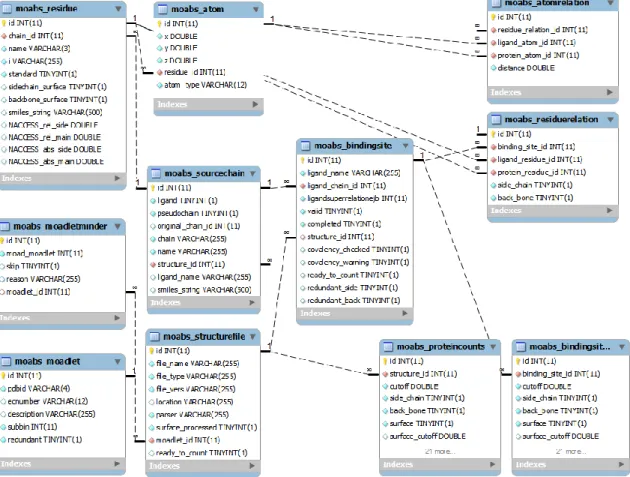
Figure II-7: Entity relationship diagram of the extension to the Binding MOAD relational object model. The schema is derived directly from the MySQL database. Tables that store the structural information are on the left. Tables that store the binding-site residue relationships are on the upper right. Tables that store pre-calculate residue-count data are on the lower right. The moabs_bindingsite table (middle of figure) provides a foreign key to the existing Binding MOAD schema. ... 53

Figure III-1: Frequencies of solvent-accessible SC residues on the protein surface with a cutoff of SASA≥5Å2 (black bars) and SASA≥0.5Å2 (white bars). Residues are sorted by decreasing hydrophobicity. ... 57

Figure III-2: Relative frequency of sc-only, BB-only or both (SC+BB) interactions per residue. The residues with “SC” interactions in our analysis combine the sc-only and “SC+BB” contacts (blue+yellow). Residues ordered by increasing BB-only frequency. Here, all Gly interactions are shown as BB-only to show its overall contribution to BB-only contacts. ... 59

Figure III-3: Frequencies of BB-only residue contacts on binding site, sorted by increasing frequency of on the protein surface. Surface residues with ≥5Å2

backbone SASA are shown. Gly interactions are shown as BB-only to stress that it constitutes the vast majority of such contacts. ... 59

Figure III-4: A) Frequencies of solvent-accessible side chains on the protein surface and in binding sites with SASA cutoff ≥ 5Å2. B) Median propensity of residues in ligand binding sites of valid and invalid ligands, analyzed across all proteins. Residues in A and B are ordered by increasing frequency on surface. C) Ratio of residue propensity for valid versus invalid binding sites. Residues ordered by decreasing ratio. Error bars in B and C indicate 95th percentiles of 10,000 leave-10%-out samples. ... 61

Figure III-5: Propensities of residue SC interactions in valid sites, with and without the top 20 ligands by frequency. A) Propensities in valid sites. B) Propensities in invalid sites. The error bars represent 95th percentile bounds based on leave-10%-out clustering within each set. Residues are ordered by increasing frequency on protein surface. ... 67

Figure III-6: A) Protein surface, B) valid binding-site, and C) invalid binding-site frequencies, and D) valid binding-site propensities of six residues. Values for subsets of

(10)

the protein structure set, from 1% to 99% of the full set, are shown with 100 samples at each percent point. ... 70

Figure III-7: Propensities in A) enzyme and B) non-enzyme valid binding sites The black error bars represent 95th percentile bounds based on leave-10%-out clustering. For context, red lines represent 95th percentile bounds of propensities from 10,000 random samples of A) 2500 random, diverse proteins and B) 1000 random, diverse proteins (as seen in Table III-4). Stars indicate residues whose median propensity value (±leave-10%-out 95th percentile error) falls outside of the 95th percentiles of the randomly-sampled propensities. ... 73 Figure IV-1: Example of an alpha sphere. The alpha sphere is displayed in red, and the three contacted atoms (2D) are in black. Figure taken from Schmidtke et al. [57] .. 79

Figure IV-2: Graphical illustration of the RO and MO criteria used for assessing a successful binding-site prediction. ... 81

Figure IV-3: Residue propensities derived from the prediction set (white) and propensity set (white) of valid ligand binding sites A) and invalid ligand binding sites B). Error bars represent 95% quartiles of leave-10%-out cross-validation sampling. ... 86

Figure IV-4: Residue propensities derived from the propensity set of valid ligand binding sites A) and invalid ligand binding sites B). Higher values highlighted in red, lower values in blue. ... 87

Figure IV-5: A) Fractions of structures in the full prediction set with respect to the number of co-crystallized ligands. B) Structures with one co-crystallized ligand, binned by heavy atom count and showing proportions of structures with various number of protein chains within bin. ... 89

Figure IV-6: Prediction success of various scores as a function of protein size. Structures with one ligand are binned by number of heavy atoms. Success rates are calculated separately for each bin. Median MO values for prediction matches in each bin are also shown. Error bars show standard deviation for SiteFinder and Valid scores in 1000 rounds of leave-10%-out sampling of the full set of 422 proteins. ... 93

Figure IV-7: Prediction success usingf consensus scores, reported as a function of protein size. Structures with one ligand are binned by number of heavy atoms. Success rates are calculated separately for each bin. Error bars show standard deviation for

(11)

SiteFinder scores in 1000 rounds of leave-10%-out sampling of the full set of 422

proteins. ... 96

Figure IV-8: Prediction success, reported as a function of protein size. Structures with one ligand are binned by number of heavy atoms. Success rates are calculated separately for each bin. Number of structures in each bin is also shown. Error bars show standard deviation for SiteFinder and Valid scores in 1000 rounds of leave-10%-out sampling of the full set of 422 proteins. ... 96

Figure V-1: Buried Surface Area (BSA) distribution for valids and invalids. ... 107

Figure V-2: Size distribution for valids and invalids ... 107

Figure V-3: Solubility (logS) distribution for valids and invalids ... 108

Figure V-4: Hydrophobicity (SlogP) distribution for valids and invalids. ... 108

Figure V-5: ROC plot showing performance of physicochemical descriptors as classifiers: Molecular Weight (MW), logS, SlogP, Buried Surface Area (BSA), percent Exposed Surface Area (%ESA), and the principal component (PCA1). Areas under the curve (AUC) are noted in parenthesis in the legend. ... 110

Figure V-6: ROC plot of ITScore performance ... 111

Figure V-7: ROC plot of DOCK4 performance ... 112

Figure V-8 – ROC plot of X-Score performance ... 112

Figure V-9 - ROC plot of AutoDock4 performance ... 113

Figure V-10 - ROC plot of Scoring Function Performance ... 113

Figure VI-1 : A) Most methods for superimposing flexible proteins are based on two steps, which involve determining a subset of related atoms and overlaying the subset using a standard RMSD-fit procedure. Each technique differs in the way that it identifies the related subsets, but in the superposition step, all of the techniques designate each Cα as “in” or “out” of the calculated fit. B) Our weighted superposition is based on all Cα. Multiple solutions can be found where the domains are reflected in the resulting weights and superpositions. Blue and green regions have high weights, align well, and define a domain. Red regions have low weights and poor agreement in the overlay. ... 123

Figure VI-2: Chaperonin family (20.8% ID). Most techniques would readily identify the similarity between the thermosome and GroEL in the similar the bound

(12)

conformation, but they may not identify its similarity with the apo conformation of GroEL. A) wRMSD superposition of the bound conformation of GroEL[210] (thick, colored lines) onto the homologous thermosome[211] (thin, black lines). Light gray regions of GroEL indicate residues within gaps in the alignment. B) wRMSD fit of the apo conformation of GroEL[210] (thick, colored lines) onto its homolog thermosome[211] (thin, gray lines). The wSUM gives the average weights of all paired residues, showing that the two bound conformations in A have greater similarity than the two conformations in B. ... 124

Figure VI-3: Median RMSD distances (measures of agreement, not overlay fit) between superpositions obtained from varying sequence alignment parameters. Standard superposition values on the x-axis are higher than the weighted superposition values on the y-axis, indicating greater variation in solutions for the sRMSD superpositions and better agreement across the wRMSD superpositions. Blue bubbles represent medians of superpositions obtained from global Needleman-Wunsch alignments; red bubbles are from local Smith-Waterman alignments. The size of the bubbles is proportional to sequence identity of the aligned protein pairs (39% to 16%) with smaller bubbles indicating less similarity. In general, the smaller bubbles show higher variation due to difficulty of obtaining a consistent initial sequence alignment. ... 129 Figure VI-4: DNA methylase family (23% ID). Weighted structural superpositions are nearly independent of the sequence alignment method, but standard superpositions are greatly affected. A) Overlays of 2ENT (black ribbon) to 1BOO[218] (colored ribbons) from standard superpositions based on seven different sequence alignments. B) The seven weighted superpositions of 2ENT to 1BOO, based on the same varied sequence alignment routines collapse into a single converged solution. ... 131

Figure VI-5: SpoU rRNA methylase family (26% ID). A) NW sequence alignment of 1IPA and 1GZ0 using default parameters. Lower case represents sequence dis-similarity, and gaps are shown with dashes. The underlined region notes domain 1, yellow represents α-helices, purple represents β-sheets, and boxes represent misaligned residues corresponding to the labeled α-helix and β-sheet in BandC. Atom pairs with a weighting of 50% or greater in the wRMSD calculation are noted with asterisks. B)

(13)

Standard superposition superpositions of 1GZ0 (colored ribbon) onto 1IPA (black ribbon) obtained using the initial alignment (from A), colored by weight. C) Weighted superposition obtained from the initial standard superposition. D) SE sequence alignment based on the wRMSD superposition, which now corrects the alignment of the secondary structure elements based on their spatial proximity in C. ... 133

Figure VI-6: Alignment results of HwRMSD (using BLOSUM50 global NW alignment) compared to other structural alignment programs using the RMSD A) and the wSUM B) metrics. Lower values of RMSD and higher values of wSUM represent a better alignment. Sequence similarity of the protein pairs decreases from left to right. ... 137

(14)

LIST OF TABLES

Table I-1: Representative algorithms for binding site prediction. ... 9

Table I-2: Notable test sets for binding-site prediction algorithms ... 24

Table II-1:Definition of unusual HET groups. For brevity, not all compounds are listed. ... 37

Table III-1: Summary data of structures from the 2009 Binding MOAD release used in the propensity calculations. Enzyme class memberships determined based on EC annotations from the PDB. All SASA areas calculated by NACCESS. ... 60

Table III-2: Composition of binding sites with respect to bound ligand for the top 20 valid ligands. Ligand listed in decreasing fraction of 5562 binding sites. Most frequently interacting residue for each ligand is in bold. ... 64

Table III-3: Composition of binding sites with respect to bound ligand for the top 20 invalid ligands. Ligands listed in decreasing fraction of 3461 binding sites. Most frequently interacting residue for each ligand is in bold. ... 65

Table III-4: Propensity median, standard deviation, and 95th percentile bounds for 6 representative residues in sampled subsets of protein structures. All values based on 10,000 random samples from the full protein set. ... 70

Table IV-1: Success rate of predictions in proteins with one co-crystallized ligand, and success rate for the same proteins if binned by protein size. ... 90

Table IV-2: Pearson correlations among the various scoring schemes. ... 91

Table V-1: Set of valid complexes. ... 104

Table V-2: Set of invalid complexes ... 105

Table V-3: Number of invalids in the top ranked results of the scoring functions. 111 Table V-4: Top scoring valids. Unique valids in italics, those scored in the top 10 by 2 or more functions in plain text. ... 119

(15)

Table V-5: Top scoring invalids. Unique valids in italics, those ranked in the top 10 by two or more functions in plain text. Invalids found in known binding sites are marked with an asterisk ... 119

Table VI-1: Median RMSD differences (in Å)* between the structural superpositions generated utilizing sequence alignments with different parameters; using global (Needleman-Wunsch) or local (Smith-Waterman) sequence alignment algorithm, and standard or weighted superposition algorithm. ... 128

(16)

ABSTRACT

Large-Scale Analysis of Protein-Ligand Binding Sites Using

the Binding MOAD Database.

by

Nickolay Khazanov

Chair: Heather A. Carlson

Current structure-based drug design (SBDD) methods require understanding of general tends of protein-ligand interactions. Informative descriptors of ligand-binding sites provide powerful heuristics to improve SBDD methods designed to infer function from protein structure. These descriptors must have a solid statistical foundation for assessing general trends in large sets of protein-ligand complexes. This dissertation focuses on mining the Binding MOAD database of highly curated protein-ligand complexes to determine frequently observed patterns of binding-site composition. An extension to Binding MOAD’s framework is developed to store structural details of binding sites and facilitate large-scale analysis. This thesis uses the framework to address three topics. It first describes a strategy for determining over-representation of amino acids within ligand-binding sites, comparing the trends of residue propensity for binding sites of biologically relevant ligands to those of spurious molecules with no

(17)

known function. To determine the significance of these trends and to provide guidelines for residue-propensity studies, the effect of the data set size on the variation in propensity values is evaluated. Next, binding-site residue propensities are applied to improve the performance of a geometry-based, binding-site prediction algorithm. Propensity-based scores are found to perform comparably to the native score in successfully ranking correct predictions. For large proteins, propensity-based and consensus scores improve the scoring success. Finally, current protein-ligand scoring functions are evaluated using a new criterion: the ability to discern biologically relevant ligands from “opportunistic binders,” molecules present in crystal structures due to their high concentrations in the crystallization medium. Four different scoring functions are evaluated against a diverse benchmark set. All are found to perform well for ranking biologically relevant sites over spurious ones, and all performed best when penalties for torsional strain of ligands were included. The final chapter describes a structural alignment method, termed HwRMSD, which can align proteins of very low sequence homology based on their structural similarity using a weighted structure superposition. The overall aims of the dissertation are to collect high-quality binding-site composition data within the largest available set of protein-ligand complexes and to evaluate the appropriate applications of this data to emerging methods for computational proteomics.

(18)

CHAPTER I

Introduction and Background

1.1

Overview

Proteins are ubiquitous in the cellular environment and are essential for biochemical functions that sustain life. To accomplish their task, proteins interact with a variety of entities in the cell, some macro-molecular (DNA, RNA, membranes) and others smaller (catalytic substrates, nucleotides, peptides, and man-made chemicals). The diverse interactions between proteins and their small molecule ligands are the focus of intense study, not only for elucidation of cellular mechanisms, but also for facilitating the design of drugs to modulate protein function in disease states. A significant portion of this design process is based upon the three dimensional structures of the protein and the ligand, in complex or separate.

The challenge of structure-based drug design (SBDD) is to correctly predict which small molecule would bind to a specific protein and what impact it might have on its function. SBDD involves an intimate understanding of how a ligand interacts with its binding site on the protein surface and using that information to predict what other ligands can bind and how strong the binding will be. Screening large databases of potential lead compounds against a structure of a protein can speed drug development by focusing the more resource-intensive experiments on a narrow set of compounds most likely to have activity.

In general, two major requirements for SBDD are the availability of a 3D structure of the desired protein target and the annotation of the ligand binding site(s) on that protein. In the recent years, SBDD received a major boost as the number of known protein structures has grown exponentially, thanks in part to numerous structural genomics projects aimed at obtaining X-ray crystal structures of proteins with unknown or poorly understood function [1]. While some contain co-crystallized ligands, most are

(19)

un-liganded. This large number of “incomplete” protein structures has raised new challenges in predicting and characterizing protein-ligand interactions. One of the more fundamental challenges is the identification of pockets on the protein surface capable of binding a small molecule. This can be a relatively straightforward process if the protein in question is a member of a well-studied family because function and binding pockets can be identified through sequence homology to an existing protein structure. However, the aim of many of the structural genomics projects is to find new uncharacterized targets, so many of the proteins in the new structures may have low sequence homology to any other structure in the Protein Data Bank (PDB) [2]. In these cases, structure-based methods need to be employed. Methods for determining the location of binding sites include computational and experimental fragment-based screening, identifying structural similarity to a known binding site, or using a structure-based prediction tool.

Once a binding site is located, the subsequent challenge is to describe the functional significance and selectivity/specificity of the site for various small molecules. While classical SBDD methods such as in silico screening can be used to determine possible binding partners, the existence of extensive databases of protein-ligand binding pockets motivates the development of comparative methods to leverage this structural data. One way to use this data is to derive a “druggability” or “bindability” score that is trained on existing protein-ligand structures. A druggability score can be used to rank identified pockets by how likely each is to bind a drug-like ligand. The ‘druggability’ index approach is relatively popular, but it has difficulty separating pockets known to bind drugs from pockets not suited to drug design, known to bind only small organic molecules. This is likely due to the high similarity of such sites and the limited dataset used to train the score [3]. Comparing one binding pocket to another to find significant similarities is a knowledge-based way to infer the ligands capable of binding to a pocket. The challenge faced by this approach is usually determining the significance of the similarity by estimating a cutoff value on a sufficiently diverse set of example complexes. These knowledge-based approaches also have the potential to address significant challenges in the drug-design process, – such as predicting off-target effect of new drugs [4], finding secondary targets for existing drugs [5], and engineering novel proteins to bind specific ligands [6]. The development of such tools requires an intimate

(20)

understanding of the variation within binding pockets across the known “pocketome” and their relative importance in partitioning the vast many-to-many interaction network of proteins and small molecules.

All of the above-mentioned challenges require methods that incorporate efficient yet informative descriptors of structural, physicochemical, and dynamic features of the protein surface. Also, they must have a solid statistical foundation for assessing similarities or differences between such regions. This dissertation focuses on mining the Binding MOAD database, a vast, curated set of protein-ligand complexes, for frequently observed patterns of binding-site composition with respect to ligand type. We then apply these patterns to the improvement of emerging binding-site prediction and comparison methods. After a short description of Binding MOAD and the extensions made to the database framework to facilitate binding-site analysis, the thesis addresses three topics. It first describes a strategy for determining over-representation of certain amino acids in ligand-binding sites. The significance of this over-representation is assessed by comparing binding pockets of biologically relevant ligands to those that bind spurious molecules with no known function. Significant trends in the propensities are described, and the effect of the data set size on the variation in propensity values is determined. Second, the propensities of residue occurrence are applied to improve the performance of a de novo binding-site prediction method. Propensity-based scores are used to rank predictions from the geometry-based SiteFinder algorithm. They are found to perform well on their own and in combination with the default SiteFinder score. The effect of predicted site size and protein size on prediction success is examined to identify cases where propensity-based scores are especially helpful.

Finally, this dissertation describes an evaluation of current protein-ligand scoring functions with a new criterion – the ability to discern biologically relevant ligands from “opportunistic binders,” molecules present in many crystal structures due to their high concentrations in the crystallization medium. A diverse benchmark of both types of complexes is compiled from the PDB and evaluated with four different scoring functions representing different scoring approaches. Particularly challenging examples are examined, such as those where biologically relevant binding is weak or invalid ligands that mimic biologically relevant contacts in a known binding site. The final

(21)

chapter presents a new method for better structural alignment of two homologous proteins based on the weighted superposition (wRMSD) technique [7]. This new HwRMSD method performs comparably to established structural alignment methods and is effectively used on proteins pairs with large structural changes. While HwRMSD does not utilize binding-site information, it has potential applications to structural comparison of ligand-binding regions. The overall aims of the dissertation are to collect high-quality data to describe the composition of binding sites within the largest available set of protein-ligand complexes and to evaluate the appropriate applications of this data to emerging methods for computational proteomics.

1.2

Understanding General Trends of Protein-Ligand binding

The understanding of protein-ligand binding has come a long way since the formulation of the lock-and-key hypothesis in 1984 by Hermann Fischer, who suggested the binding of a substrate to an enzyme is analogous to a key being inserted into a lock. This model of shape complementarity between the ligand and the receptor has since expanded to incorporate the flexibility of the receptor. More dynamic models of binding include the zipper model, the induced-fit model, and the conformational-selection model (reviewed in [8]). Considering that a majority of structural knowledge of proteins still comes from static structures obtained by x-ray crystallography [1] or homology modeling [9], it is still a challenge to identify binding regions that might only be present in certain protein conformations, yet are important for the function of the protein. Geometric complementarity is required but not sufficient for ligand binding [10]. Molecular recognition also relies on physicochemical complementarity – namely the various electrostatic, hydrogen-bonding, hydrophobic, and solvent-mediated interactions between the protein and the ligand. All of these features must combine to create an energetically favorable interaction for the ligand to enter and remain in the binding site long enough to affect protein function. Despite major efforts to develop computational methods that can describe these physicochemical interactions from “first principles” using sophisticated force-fields, a large portion of existing methods rely on knowledge-based or empirical approaches.

(22)

The knowledge-based methods are fast and efficient, but they suffer from over-reliance on their training sets, which can limit their generalizability [11]. Empirical methods parameterize their energy-estimation functions with existing protein-ligand data, and thus, offer an intermediate approach. However, none of these methods have been very effective in predicting experimentally-determined ligand affinities [12], illustrating the challenges inherent in understanding the full range of factors governing protein-ligand binding.

1.2.1 Binding-Site Shape

Looking at the variation of shapes, sizes, and composition of protein-ligand binding sites and the ligands they bind, it is easy to see why finding a general method for predicting their location and binding partners is such a challenge. Recent studies of thousands of human protein-ligand complexes found a complicated relationship between the similarity of protein sequences and the similarity of their pockets and bound ligands [13-15]. By clustering the proteins, ligands, and pockets separately, one study found many examples of highly related proteins binding varied ligands. Conversely, many ligands similar in structure, as measured by Tanimoto similarity, have unrelated protein partners, as measured by sequence similarity [13]. Moreover, it has been observed that binding sites of two proteins can be similar despite having different global folds [16], which is likely a result of convergent evolution.

The shapes of binding pockets range from small spherical invaginations to deep curved or linear clefts in the protein [17]. Catalytic sites are usually situated at the bottom of the deeper clefts, where hydrophobic residues can shield the catalytic residues from solvent while the latter perform the enzymatic reaction. However, other functional sites can vary greatly in size and depth. To complicate matters, the size of the binding site is not necessarily related to the size of the ligand it can accommodate [10, 18], and several binding regions can exist in close proximity, forming a large swath of ligand-binding surface with complex geometry. The average volume of a drug-binding pocket is between 600 - 900 Å3, depending on the method used to delineate pocket boundaries [19-21], while that of a drug-like ligand is around 400Å3. Since drug molecules are often designed to be as small as possible to improve their bioavailability,

(23)

this range of binding site and ligand volumes only increases when the full variety of biologically-relevant protein-ligand complexes is considered. Despite the variation, some general trends have emerged from the recent studies. Ligands, and especially drugs, have been observed to bind into the largest and/or deepest concavity on the protein surface [18]. On average, that cavity might be three times as large as the ligand, indicating the presence of a large ”buffer” zone between the ligand and protein [10] and demonstrating the difficulty in defining the boundaries of what really constitutes the binding site.

1.2.2 Binding-Site Composition

Chemical complementarity may have general trends as well. In a study of ligand efficiency in enzymes and non-enzymes, high-affinity enzyme ligands were observed to be larger than those with low-affinity, indicating increasing ligand size can improve affinity. However, non-enzymes were observed to have high ligand efficiencies irrespective of ligand size, and the composition of their binding sites had greater influence upon modulating affinity [22]. Such relative trends between protein classes are helpful in guiding SBDD with a particular protein target in mind, but provide only broad-brushstroke insight into binding-site behavior. Many methods that delve into the details of the protein-ligand interactions have been developed to score potential matches between a specific ligand pose and its receptor [23-26]. These knowledge-based scoring functions look for general trends of atom-atom contacts between ligand and protein in large structure databases, and they reward frequently-seen interactions in the potential protein-ligand pair to be scored. Depending on the training set, the interaction trends captured by the function may not be generally transferable to a wide variety of proteins [27]. Moreover, the trends utilized by the scoring functions require the presence of both protein and ligand atoms in a structure. They are usually applied in cases where the relative location of the binding site has been narrowed down, and only the best binding mode is sought [28]. This limits their usefulness in understanding general trends of binding-site composition in the absence of a potential ligand.

(24)

Yet another class of studies has analyzed the composition of protein surfaces in general. This led to general insight that a mix of both hydrophobic and hydrophilic solvent-exposed residue exist on protein surfaces [29], and that there is limited correlation between residue hydrophobicity and its surface exposure patters [30] (i.e., its presence on the surface). Such insights further the understanding of the composition of protein surfaces, but they do not compare and contrast their findings with the regions of protein surface involved in ligand binding.

With the advent of thousands of protein-ligand complexes in the PDB, analyses of composition and conservation of residues in ligand binding sites are becoming more common. Such studies take a more asymmetric view of the protein-ligand interactions, focusing on the trends in protein composition independently of the details of ligand interaction. The trends are often linked back to significant or frequently observed interactions, but they can also be used to contrast ligand-binding regions of the protein to the rest of the protein surface or assign some manner of scores to protein residues in a structure without co-crystallized ligand.

One of the most detailed studies of ligand-interacting residues was carried out by Bartlett et al. on ~200 enzyme active sites [31]. A residue’s role in enzyme catalysis was confirmed by manual curation. His, Cys, Asp, and Arg were found to have the highest catalytic propensities (over-representation in catalytic site as compared to the rest of the protein). A variety of other detailed trends for the solvent exposure and biochemical function of the residues were also determined. The study provided a heuristic basis for predicting catalytic residues in enzymes, and it was the source for the Catalytic Site Atlas database. However, the focus on catalytic residues side-stepped the analysis of residues involved in non-catalytic interactions with the ligand. These residues likely provide energetically-favorable interactions that maintain the ligand in the correct binding mode while the catalytic residues perform their function; therefore, they are important to include in residue composition analysis.

A recent study by Davis and Sali examined the general residue composition of ligand-binding sites as compared to protein-protein binding sites and the protein surface with no known interactions [32]. They found residue composition in protein-protein binding sites resembles that of the general protein surface, while residues in

(25)

protein-ligand binding sites had much different propensities. Residues involved in both protein and ligand binding (bi-functional) showed intermediate propensities. Largest propensities for ligand-binding sites were seen for Cys, Phe, His, Met, Trp, Val, and Ile residues. Cys, Ile, and Val were unique with respect to protein-protein or bi-functional positions. That study analyzed ~35,000 binding sites, but it was based on only ~1000 domain families, which is a very redundant set of structures.

A more focused study by Nayal and Honig extensively characterized the binding sites of 99 non-redundant, protein-ligand complexes as part of an effort to develop a binding-site detection algorithm [18]. Unfortunately, the authors focused on classification of binding sites as being drug-binding or not, and they did not report general trends of the binding pockets analyzed in the study. However, they found that Asn, Gln, and Glu were important residues in recognizing drug-binding sites among a set of sites binding various ligands. Aside from these representative efforts, relatively few surveys of large sets of protein complexes have been completed [33-37], and the ever-growing number of raw structural data and binding-site characterization methods promise greater insights into the general theories governing protein-ligand complexes. These insights will undoubtedly lead to improvements in SBDD strategies that make use of these theories [36, 38].

1.3

Methods to Identify Binding Sites

de novo

Methods that aim to predict binding sites face several major challenges. Two of the largest are the change in the binding-site structure upon ligand binding (an implication of the induced-fit model of ligand binding) and the sheer variety of existing binding-site shapes and sizes needed to accommodate the various biologically-relevant ligands. Another challenge is detecting sites located at protein subunit interfaces, which are often omitted in the test sets used to develop and benchmark prediction methods. Even with a large and properly chosen evaluation set, there remains the challenge of precision and accuracy, i.e., identifying the precise region expected to bind a ligand without over-predicting. Overpredicting is problematic because classifying the entire surface of a protein as a binding site would certainly result in a match, so evaluating the success of a prediction must be done carefully. The field as a whole still lacks gold-standard sets or

(26)

consistent metrics for calling “true” predictions. These challenges will need to be overcome for successful application of prediction methods in SBDD, which require a precise and accurate definition of the binding site to focus the search effort on relevant areas of the protein and reduce false-positive results.

Three major classes of tools have emerged to address binding-site prediction: 1) those that use the geometry of the protein surface to identify large concavities resembling a binding site, 2) those that use probe-based methods to identify regions of the surface capable of making energetically favorable interactions with a potential ligand, and 3) those that use knowledge-based methods to search a protein structure against a database of known binding sites. Representative tools in these categories are discussed below and summarized in Table I-1. Additional tools exist that use more complex methods, such as molecular dynamics, to identify the binding regions, but they are outside the scope of the current discussion.

Table I-1: Representative algorithms for binding site prediction.

Pub Date

(Latest) Type Server Download

Open Source GRID ₁₉₈₅ _Energy-based POCKET ₁₉₉₂ _Geometric VOIDOO ₁₉₉₄ _Geometric _✓ APROPOS ₁₉₉₆ _Geometric PASS ₂₀₀₀ _Geometric _✓ eF-Site ₂₀₀₂ _{Knowledge-based} _✓ Pocket-Finder ₂₀₀₅ _Geometric _✓ _✓ PocketFinder ₂₀₀₅ _Energy-based _✓ _$ SiteFinder ₂₀₀₅ _Geometric _$ Q-SiteFinder ₂₀₀₅ _Energy-based _✓ ProFunc ₂₀₀₅ _{Knowledge-based} _✓ ConSurf ₂₀₀₅ _{Knowledge-based} _✓ SiteEngine ₂₀₀₅ _{Knowledge-based} _✓ LIGSITEcsc ₂₀₀₆ _{Geometric/Genomic} _✓ _✓ _✓ SURFNETConSurf ₂₀₀₆ _{Geometric/Genomic} _✓ _✓ _✓ CAST(p) ₂₀₀₆ _Geometric _✓

(27)

SCREEN ₂₀₀₆ _Geometric _✓ Pocket-Picker ₂₀₀₇ _Geometric _✓ _✓ PHECOM ₂₀₀₇ _Geometric SiteMap ₂₀₀₇ _Combination _$ CavBase ₂₀₀₇ _{Knowledge-based} _✓ PocketDepth ₂₀₀₈ _Geometric _✓ FINDSITE ₂₀₀₈ _{Knowledge-based} _✓ Fpocket ₂₀₀₉ _Geometric _✓ _✓ _✓ McVol ₂₀₁₀ _Geometric _✓ _✓ PROSITE ₂₀₁₀ _{Knowledge-based} _✓ ProBiS ₂₀₁₀ _{Knowledge-based} _✓

1.3.1 Methods Primarily Using Geometry of Static 3D Protein Structures

The earliest methods developed for prediction of surface pockets employed a grid-based approach, scanning the protein along grid lines using a geometric probe and detecting the regions where grid points lay outside of protein atoms (Figure I-1). In POCKET [39], the specific pockets were defined by protein-solvent-protein events, which are characterized as a series of grid points along the scan axes that alternate between being “inside” the protein to “outside” of the protein. Since this approach is sensitive to the relative orientation of the protein to the grid axes, it was extended in LIGSITE [40] to include scans along grid diagonals. LIGSITE was tested on a set of only 10 proteins in its initial publication, but at the time, it was a state-of-the-art method in terms of accuracy and efficient implementation. Owing to its success, it was further extended to incorporate the Connolly protein surface [41] in order to count surface-protein-surface events instead of protein-solvent-protein events. Recently, non-structural information was incorporated by considering the conservation of residues in the identified pockets. [42]. The extended version is named LIGSITEcsc. It was validated on a large set of 210 structures, which included a subset of matched apo and holo protein structures. It showed an improvement in top-ranked successful predictions from 67% to 75% as compared to LIGSITE. LIGSITE was also implemented as Pocket-Finder for comparison to energy-based methods [43].

(28)

Figure I-1: Illustration of several methods utilizing protein-structure geometry for binding-site identification. Each illustration is taken from the publication describing the respective algorithm.

(29)

LIGSTE served as a basis for the PocketPicker method, which used a finer grid representation and calculated an additional “buriedness” measure for grid points in the identified pockets [44]. The PocketPicker method performed worse (59% for top-hit success) than LIGSITE or LIGSITEcsc on the same test set of 210 complexes, a fact the authors attributed to the optimization of PocketPicker to identify smaller, more buried pockets useful for shape comparison. However, it did outperform alternative geometry-based methods PASS and SURFNET (see below). Conceptually, grid-geometry-based methods have limits due to their sensitivity to grid size, protein orientation, and the inability to define a cavity “ceiling” to delineate the outer limit of a pocket. VOIDOO was an early method that sought to rectify the limitations of grid-based approaches by detecting cavities through the expansion of atomic van der Waals (vdW) boundaries [45]. The premise was that deep pockets can be delineated by progressively expanding the vdW radii of all protein atoms until invaginations on the surface of the protein get “pinched off” by the vdW surfaces colliding at the narrowest point, i.e. the “mouth” of the pocket (Figure I-1). Although the method provided a way to outline the cavity and measure its volume independent of a grid, it could not detect shallow or broad pockets that cannot be closed off by increasing the vdW radii.

A slightly different use of grids was recently proposed in the PocketDepth method [46]. It uses the fine grid of points placed on a protein to calculate pair-wise measures of depth between pairs of points flagged as being on the surface of the protein. The points are identified as being on the surface by considering the density of protein atoms in the vicinity of a point. Depth measurements passing through a protein atom are not considered. Subspaces of the grid are evaluated based on the density and magnitude of the depths measurement among the points in the subspace. Complex clustering and filtering steps allow the algorithm to identify grid subspaces that have large numbers of ‘deep’ points in close spatial proximity, and thus delineate the predicted pocket shape based on these subspaces. The algorithm was extensively evaluated on a set of 1091 proteins from the PDBBind database [47], where it achieved a success rate of 55% among its top-ranked predictions. This performance was similar to or better than LIGSITECSC and Q-SiteFinder methods, respectively, based on the benchmark datasets for those methods (see below).

(30)

An early, alternative geometry-based method was implemented in SURFNET [48], which used an algorithm that fits spheres of varying size between all pairs of relevant protein atoms to find the pocket-like cavities. The radius of a sphere placed between several atoms is iteratively reduced until no overlap with protein atoms is achieved (Figure I-1). All indentations on a protein are packed with spheres of radii varying from 1 to 4 Å, defining the outlines and volumes of prospective binding sites. Ranking the pockets by size, SURFNET was found to correctly predict the ligand-binding pocket in 83% of the top-ranked results for a set of 67 enzyme complexes [49]. In a more recent test on 210 bound complexes from Huang & Schroeder, SURFNET underperformed in relation to LIGSITE and PASS methods, achieving a success rate of only 42% for its top-ranked predictions [42]. SURFNET was later expanded to SURFNET-ConSurf, which incorporates evolutionary sequence information to trim the predicted pocket size based on the conservation rate of its component residues.

The PASS method [50], whose top-ranked predictions achieved a performance of 54% in the Huang et al. evaluation on 210 complexes, is another popular tool that uses a probe-packing algorithm to detect protein pockets. In this algorithm, probes are packed on the protein surface so that each probe touches a triplet of adjacent protein atoms. Probes that clash with protein atoms are then removed, and the remaining probes are filtered by their degree of burial, estimated from the count of protein within 8 Å of the probe. Subsequent rounds of packing build up additional layers of probes until no more buried probes can be placed. The probes are clustered into “active site points” that define the predicted pockets. PASS was originally evaluated on 32 complexes, where its top-predicted pockets successfully identified 60% of the known sites, and on a set of 21 apo structures, where the success rate was 57%. A more recent method, PHECOM, used two sets of large and small spheres to pack the protein surface, and determined pockets by identifying small spheres that packed between the surface and the large spheres [20]. Probe packing methods might have difficulty detecting wide cavities, which would require very large spheres to define, and would limit the accuracy of pocket-volume estimation based on sphere volumes.

A series of algorithms utilize Voronoi diagrams [51] and Delaunay triangulation [52] for geometric surface representation. These techniques effectively “shrink wrap”

(31)

the protein surface in a mesh of triangles and allow for complex geometric algorithms to calculate various shape properties of this tiling. APROPOS [53], one of the earliest methods in this category, creates a Delaunay representation of the protein and then generates an α-shape, which is conceptually similar to rolling a probe with a radius α to erase edges of the Delaunay triangles. The vertices of the triangles are located at atomic centers and unaffected by the rolling-probe step. By varying the α parameter, a series of surfaces can be generated, with the most extreme value (α = ∞) generating a convex hull of the protein. Pockets of various sizes can be detected by comparing the shape of the convex hull to the alpha shapes generated by alpha values corresponding to the radii of an oxygen atom or a methyl group. The algorithm initially achieved a 95% success rate in its initial test on 200 monomer complexes, but it has not been extensively compared to other methods. CAST is a similar method that combines the Delaunay representation with discrete flow theory to identify concave pockets [35]. It first identifies the alpha-shape of the protein and defines Delaunay triangles with one or more omitted edges as “empty”. The neighboring empty triangles are then combined in the “discrete-flow” method to define continuous voids on the protein surface (Figure I-1). An obtuse empty triangle flows into its neighbor, while an acute empty triangle acts as a sink to collect the flow of its neighbors. If the flow is directed out of the protein the pocket is ignored, otherwise it is considered a putative binding site. The algorithm was tested on the 51 of the 67 proteins used by SURFNET, and it achieved a success rate of 74% (lower than SURFNET). However, the authors determined that the differences in nature of the pockets predicted by the two methods prevent fair comparison. The α-shape and secrete flow approaches might be limited in their applicability to very open pockets, since they are optimized to detect pockets whose “mouth” is smaller than the cross sections through the rest of the pocket [54]. Alpha-sphere methods, discussed below, are less sensitive to such pocket geometry.

More recent methods utilizing a surface-based approach include Fpocket [55] and SiteFinder [56]. Both use the concept of α-spheres [54] andVoronoi tessellation of the protein. An alpha sphere is a sphere contacting four protein atoms but no internal atoms (Figure I-1). Centers of alpha spheres correspond to the vertices of the Voronoi tessellation of the protein, and both Fpocket and SiteFinder algorithms determine the set

(32)

of alpha spheres based on this tessellation. Since alpha-sphere radii scale with the curvature of the plane of the four atoms they contact, small alpha spheres are located in tightly packed areas of the protein while those with larger radii are located in cavities towards the surface. Thus, clusters of alpha spheres with a desired range of radii can be used to identify and define surface cavities. Fpocket clusters the spheres by proximity, density, and size. It then prunes uninteresting sphere clusters based on cluster size and some basic definitions of polarity with respect to the atoms the spheres touch. The sites are then ranked according to a scoring scheme that estimates the “bindability” of the site based on a set of geometric and physicochemical pocket descriptors. SiteFinder performs similar clustering and pruning based on the solvent exposure of the spheres and the hydrophobicity of the neighboring atoms. Clusters with at least one “hydrophobic” sphere are retained while the rest are discarded. Fpocket was tested on the smaller bound/unbound test set of structures used by PocketPicker (see above). It outperformed PocketPicker, LIGSITEcsc, CAST, PASS, and SURFNET on the bound set of 48 structures, with an 83% success rate among its top-ranked predictions [55]. On the unbound set of the same proteins, it performed as well as PocketPicker, achieving a 69% success rate. It slightly underperformed compared to LIGSITEscs (71% success). In a recent large-scale comparison on a dataset of several thousand apo and holo structures, Fpocket performed similar into SiteFinder on the bound structure set, achieving top rank success of around 78%, compared to SiteFinder’s 77%. However, it significantly underperformed on the unbound set, where it achieved a success rate of only 42% versus 62% achieved by SiteFinder [57].

Another way of defining a protein surface is by a rolling-sphere approach. The SCREEN method uses differences in two molecular surface representations of the protein to define protein cavities [18]. First a “tight” molecular surface is constructed by rolling a small sphere (1.4Å in radius) over the whole protein. Then, a low-resolution envelope surface is constructed by rolling a sphere closer in size to a ligand molecule (5.0Å in radius). The depth of the molecular surface is then computed with respect to the envelope surface, and cavity surfaces are defined as contiguous regions of the molecular surface that are below a certain depth. A sophisticated clustering method then merges continuous cavities to produce well-delineated, compact, predicted pockets.

(33)

This is the extent of the geometric component of SCREEN, which was further used to train a classifier for predicting druggability of the sites based on an array of physicochemical proteins of the predicted pockets.

Geometric methods are relatively simple and efficient, but they have no underlying physical meaning. The following section describes representative methods that apply a more physicochemical approach, or a combination of geometric and physical features, to scan the protein surface for potential ligand-binding sites.

1.3.2 Methods Primarily Using Energetic Mapping of 3D Protein Structure

Methods that evaluate the interaction energy between the protein and a chemical probe, fragment, or molecule, to determine favorable regions date back as early as 1985, when the GRID method was first published [58]. GRID calculates interaction energies between the protein atoms and probes placed on a grid superimposed on the protein. The interaction energy is composed of Lennard-Jones, Coulombic, and hydrogen-bonding terms, and the probe identity can be varied to represent different chemical fragments. The method was designed to identify regions of interest on the protein but not necessarily predict binding sites; as such, it generates a map of the protein surface as opposed to a set of pocket predictions. Although used heavily and successfully in SBDD of individual protein targets [59], it has not been extensively evaluated as a binding-site prediction algorithm. Probe interaction energies have been successfully combined with some measure of protein geometry in the recently-developed Q-SiteFinder [43]. The Q-Q-SiteFinder algorithm relies on the GRID force field to calculate vdW interaction energies between the protein atoms and methyl probes placed on a fine grid. An interaction energy threshold is used to retain the most favorable probes. A clustering algorithm groups the probes according to their spatial proximity along the protein surface and uses the total interaction energy of the probes in a cluster to rank them relative to one another. The most favorably interacting clusters are presented as the predicted binding pockets. Q-SiteFinder was evaluated on a set of 134 proteins from the GOLD docking test set [60] and achieved a success rate of 71% in the top-ranked predicted sites [43]. The method also outperformed LIGSITE (as implemented in Pocket-Finder), which achieved a success rate of 48%. When evaluated on a set of 35

(34)

proteins with corresponding apo and holo structures, the Q-SiteFinder success rate in the top-ranked sites decreased from 80% in the bound structures to 51% in the unbound structures [43].

Shortly after the publication of Q-SiteFinder, an alternative energy-based method was proposed in PocketFinder [13] (not to be confused with Pocket-Finder, an implementation of LIGSITE). Like previous grid-based methods, PocketFinder calculates a grid potential map of vdW interaction energies using an implementation of the Lennard-Jones potential. The method deviates from its predecessors by smoothing this potential map to emphasize continuous regions of highly favorable vdW potential and then contouring the map at a level sufficient to identify putative ligand envelopes. Small envelopes are pruned, and the rest are ranked by their volumes. PocketFinder was tested on the largest set of any other method (5,616 bound and even more corresponding un-bound structures). It was found to perform better in predicting sites from ligand-bound structures than unligand-bound structures. Since the authors chose to stratify their predictions by a site-coverage threshold, a direct measure of top-rank results is not available.

A more sophisticated approach similar to GRID and Q-SiteFinder is implemented in SiteMap, part of the Schrödinger software suite [61]. SiteMap first identifies potential sites by placing a grid of probe points over the protein and retaining those that are located “outside” of the protein, have a certain degree of enclosure, and obtain favorable vdW interaction energy with the protein. An agglomerative clustering step then groups the points by proximity, and point groups are further merged if an un-interrupted point-to-point traversal can be completed from one group to the other without encountering the protein. The predicted sites are then scored and ranked according to variety of aggregate physicochemical descriptors including size, enclosure, solvent exposure, tightness of non-bonded interactions, hydrophobicity, and hydrogen-bonding potential.

Energy-based methods tend to be much faster than geometric ones, but they are more sensitive to missing atoms and proper set-up of the protonation states and atom types of each protein [57]. Alternative energy-based methods include the fairly explicit and expensive computational solvent-mapping approaches [62, 63] and whole-protein

(35)

“blind docking” methods such as MEDock [64] or an AutoDock-based method by Hetenyi et al. [65]. The former involve simulation of the protein surrounded by a bath of organic solvent to identify solvent-binding hot-spots. The later are based on existing docking and molecular dynamics software. Thus, both are beyond the scope of this introduction.

1.3.3 Methods Using Knowledge-Based Approaches to Identify Binding Sites

Knowledge-based methods used to predict ligand binding sites are comparative by definition. They make use of existing binding-site data obtained from X-ray and NMR experiments, biochemical data from site-directed mutagenesis studies, and sequence information associated with these data sources. Comparison of global or local structure of a protein of unknown function against existing databases of binding sites is the primary method for inferring the presence and/or function of the binding site. Sequence conservation or estimation of favorable energetic potentials is sometimes used to supplements the structural match. Unlike geometry- or energy-based methods, which report rank-ordered predictions, knowledge-based methods search against a large database of a known size, and then estimate the absolute statistical significance of their predictions. However, the obvious limitation of these methods is the difficulty of working with proteins that show little structural or sequence similarity to existing protein families. The power of knowledge-based methods will continue to improve as current sources of protein-structure data continue to grow.

There is an important distinction between predicting a binding site region on the surface of an uncharacterized protein and classifying the function of that region. Geometry-based and energy-based methods described in the previous sections focus on identifying the ligand-binding region, not on its classification. Although geometry-based methods such as SCREEN [18] follow up the binding-site identification step with a classification step, this classification step often relies on broadly-applicable binding-site properties to label the predicted regions as “druggable” or “bindable.” In contrast, knowledge-based prediction methods compare a potential binding region to sites of known function, and consequently, try to assign a more specific functional class to their queries. Some knowledge-based methods that are considered binding-site prediction

(36)

methods are actually binding site classification or comparison methods that rely on a geometry- or energy-based algorithm for predicting potential cavities to be used in querying known sites. For example, the popular Cavbase [66, 67] method actually relies on the geometry-based LIGSITE [68] cavity-prediction method to identify the potential pockets. The ProFunc [69] database uses the SURFNET [48] method to identify potential cavities. These predictions are then used for comparison to known ligand pockets using geometric and physicochemical criteria. The overview of the knowledge-based methods below focuses on the predictive aspect of these approaches. Binding-site similarity assessment is a broader extension of these methods that is outside of the scope of this chapter.

Evolutionary analysis can help identify patches of conserved residues on the protein surface that are essential to protein function. Conservation of residues in a family of proteins is obtained by a multiple-sequence alignment (MSAL), where family members are chosen by functional similarity, presence of a common ligand, or structural similarity. The Rate4Site method developed by Pupko et al. uses MSALs to estimate the rate of evolution among homologous proteins; it then maps the conservation data onto the 3D surface of the query protein [70]. Patches of conserved residues are assumed to have functional significance, but the interpretation of the specific binding-site location is left to the user. Bayesian inference used for the conservation calculations provides robust conservation scores that can differentiate highly conserved positions arising due to short divergence times between proteins, from less-conserved positions that deserve attention due to their relatively small changes across long phylogenetic lineages [71]. The ConSurf database uses the Rate4Site method to identify functionally important amino acids on a query protein surface by searching a large database of protein sequences to generate MSALs appropriate for estimating residue conservation. The self-professed bottleneck of this class of methods [72, 73] is the availability of sufficient sequence data. Too little variation in the MSAL due to insufficient diversity or too few sequences (usually < 10) can severely undermine the meaningful interpretation of the evolutionary relationships [74].

The PROSITE database also relies on sequence conservation to detect functionally important regions in proteins of unknown function [75]. It attempts to counteract the

(37)

problems of insufficient sequence homology or small family size by considering short (10-20 residues), conserved sequence motifs in addition to full-length sequence profiles. A query sequence can be analyzed for the presence of a motif even it has no significant pair-wise sequence homology to known proteins. The short motifs can be constructed from full length MSALs in functionally-related proteins, such as enzymes or proteins containing prosthetic groups. Due to their size, individual patterns are not sufficient to