FOUR CLOSURE STRUCTURES PROJECT
Summary Report of Findings and Recommendations
Lafayette 135 Regency Square Lafayette, LA 70508 P. O. Box 52106 (70505) 337.237.2200 phone 337.232.3299 fax New Orleans 1100 Poydras, Suite 1550 New Orleans, LA 70163 P. O. Box 57089 (70157-7089 504.582.2201 phone 504.582.2210 fax Baton Rouge 445 North Blvd, Suite 601 Baton Rouge, LA 70802 225.344.6701 phone 337.232.3299 fax Houston
675 Bering Drive, Suite 260 Engineers • Surveyors
Prepared For:
Coastal Protection and Restoration Authority
Iberia and Vermilion Parishes
TABLE OF CONTENTS
1.0 INTRODUCTION ... 1 2.0 PREVIOUS MODEL ... 1 3.0 DATA COLLECTION ... 3 4.0 FENSTERMAKER MODEL ... 3 4.1 Model Validation ... 6 5.0 RESULTS ... 95.1 Scenario 1: South Structures with 2010 Tides and 2010 Channel Discharges ... 10
5.2 Scenario 2: South Structures with 2010 Tides, 2010 Channel Discharges, and Large Atchafalaya Discharge ... 13
5.3 Scenario 3: South Structures with 2010 Tides, 2010 Channel Discharges, and 50-year Rainfall Event ... 16
5.4 Scenario 4: Inland Structures with 2010 Tides, 2010 Channel Discharges, and 50-year Rainfall Event ... 20
6.0 DISCUSSION AND CONCLUSION ... 21
7.0 REFERENCES ... 22
APPENDICES
APPENDIX A: Model Input Data
APPENDIX B: Water Surface Elevation and Salinity Comparison APPENDIX C: MIKE FLOOD Solver Routines
LIST OF FIGURES
Figure 1-1: Four Closure Structures Project Map ... 1
Figure 2-1: Chenier Plain Model Domain ... 2
Figure 4-1: Fenstermaker Model ... 4
Figure 4-2: Channel Bathymetry Collection Effort ... 5
Figure 4-3: Channel Cross-sections Comparison at Locations North of the GIWW ... 5
Figure 4-4: Validation Locations ... 6
Figure 4-5: CRMS-531 Hourly Water Surface Elevation Validation ... 7
Figure 4-6: CRMS-531 Daily Salinity Validation ... 7
Figure 4-7: CRMS-532 Hourly Water Surface Elevation Validation ... 7
Figure 4-8: CRMS-532 Daily Salinity Validation ... 8
Figure 4-9: NOAA 8765251 Hourly Water Surface Elevation Validation ... 8
Figure 4-10: NOAA 8765251 Daily Salinity Validation ... 8
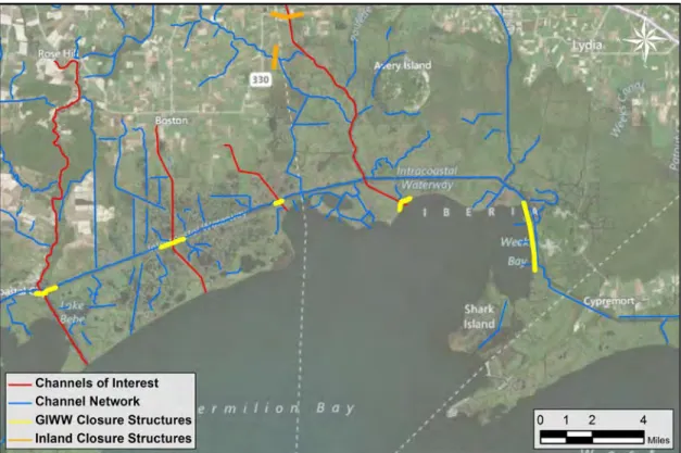
Figure 5-1: Closure Structure Locations ... 9
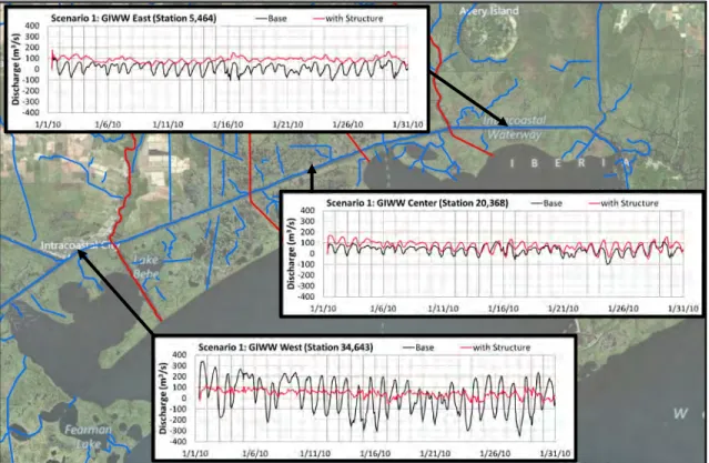
Figure 5-2: Scenario 1 GIWW Discharge Comparison ... 10
Figure 5-3: Scenario 1 Water Level Comparison ... 11
Figure 5-4: Scenario 1 Salinity Comparison ... 12
Figure 5-5: Scenario 2 GIWW Discharge Comparison ... 13
Figure 5-6: Scenario 2 Water Level Comparison ... 14
Figure 5-7: Scenario 2 Salinity Comparison ... 15
Figure 5-8: Scenario 3 GIWW Discharge Comparison ... 16
Figure 5-9: Scenario 3 Water Level Comparison ... 17
Figure 5-10: Scenario 3 Salinity Comparison ... 18
Figure 5-11: Scenario 3 Maximum Water Level Comparison over 15 Days ... 19
Figure 5-12: Scenario 3 Maximum Salinity Comparison over 15 Days ... 19
Figure 5-13: Scenario 4 Closure Structure Locations ... 20
Figure 5-14: Scenario 4 Water Level Comparison ... 21
Figure 5-15: Scenario 4 Maximum Water Level Comparison over 15 Days ... 22
LIST OF TABLES Table 3-1: Chenier Plain Model Inputs ... 3
1.0
INTRODUCTION
Fenstermaker teamed with the Coastal Protection and Restoration Authority (CPRA) and ARCADIS to examine water level and salinity impacts due to channel closure structures placed in Vermilion and Iberia Parishes. The goal of this Four Closure Structures project was to develop numerical simulations to evaluate impacts of the closure structures during storm events. Fenstermaker refined an existing MIKE FLOOD model to analyze the Vermilion Bay vicinity (Figure 1-1). This area is influenced by tides in Vermilion Bay and freshwater inflows from the inland riverine network.
Figure 1-1: Four Closure Structures Project Map
2.0
PREVIOUS MODEL
Fenstermaker refined an existing MIKE FLOOD model of coastal Louisiana developed under the Louisiana Coastal Area (LCA) Science and Technology Office in conjunction with the University of Louisiana at Lafayette. This Chenier Plain model analyzed regional tidal and salinity circulation
model began in 2006 examining water levels, salinity, and velocity patterns on a daily and monthly scale along the Louisiana coastal zone from Freshwater Bayou to Sabine Lake (Figure 2-1).
The Chenier Plain model is a living model that has been calibrated and validated over multiple years (Meselhe and Miller 2007), and is regularly updated with improved data and modeling techniques. The most recent version of the Chenier Plain model was expanded to include Vermilion Bay and 5,100 square kilometers of additional open water in the Gulf of Mexico, in addition to hydrologic data from 2010. The 2010 model was validated and calibrated using gage data collected by CPRA and the National Oceanic and Atmospheric Administration (NOAA). In addition to the reasons stated above, Fenstermaker selected the 2010 Chenier Plain model for the Four Closure Structures study because of Fenstermaker’s familiarity of the model setup and outputs.
Figure 2-1: Chenier Plain Model Domain (Meselhe and Miller 2007)
The MIKE FLOOD software suite developed by the Danish Hydraulic Institute (DHI) was selected for the Four Closure Structures study because of its coupled one- and two-dimensional capabilities and ability to capture time varying hydraulic structures such as locks. MIKE FLOOD is an ideal software suite for analyzing channel, open water, and overland flow in conjunction with
salinity transport. Please see Appendix C for a detailed discussion on the MIKE FLOOD solver routines (Meselhe and Miller 2007).
3.0
DATA COLLECTION
The Chenier Plain model was developed in 2007 using data from 2002 through 2006. As a living model, it has been continuously expanded and updated as more data becomes available. The data types and sources listed in Table 3-1 were collected as boundary conditions for the 2010 Chenier Plain model. Time series of select data are located in Appendix A.
Table 3-1: Chenier Plain Model Inputs
Type Source
Bathymetry National Geophysical Data Center (NGDC)
Evapotranspiration NOAA & Louisiana State University (LSU) AgCenter
Hydraulic Structures United States Army Corps of Engineers (USACE) & Coastal Wetlands Planning and Protection Act (CWPPRA) Precipitation USACE, National Climatic Data Center (NCDC), & United States Geological Survey (USGS) Riverine Discharge USGS & NOAA
Salinity USGS, Coastal Protection and Restoration Authority (CPRA) Coastwide Reference Monitoring System (CRMS), & USACE Topography LSU Atlas
Water Level USACE, CPRA CRMS, NOAA, & USGS Wind National Data Buoy Center (NDBC)
4.0
FENSTERMAKER MODEL
Fenstermaker was tasked with analyzing impacts to water levels and salinity in Vermilion Bay and surrounding project area due to placement of closure structures along several channels during typical conditions such as daily tide cycles and large rainfall events. ARCADIS analyzed storm surge impacts using the coastal circulation and storm surge model ADCIRC. The eastern portion of the 2010 Chenier Plain model was used to develop the Four Closure Structures model. Approximately 470 kilometers of channel and 5,600 square kilometers of model domain were added to capture water levels and salinities north of Vermilion Bay (Figure 4-1). Model
Several closure structures were placed within the model domain along Vermilion River, Boston Canal, Oaks Canal, and Delcambre-Avery Canal to reduce inland inundation due to storm surge. These closure structures would be closed before storm events reached the Vermilion Bay area and re-opened as soon as possible after the storm event to reduce flooding
Figure 4-1: Fenstermaker Model
Accurate channel dimensions were an important component of the Four Closure Structures model. Discharge is highly sensitive to channel geometry, and salinity transport is predicated on discharge. As such, a handheld depth finder was used to record water depth at locations shown in Figure 4-2. These water depths were related to observed water levels from the USGS gage at Cypremort Point and converted to an elevation. Figure 4-3 shows a comparison of channel cross-sections north of the Gulf Intracoastal Waterway (GIWW). Due to the absence of a complete survey, channels dimensions were adjusted for several channels during the validation process (orange channels in Figure 4-2). These channel dimensions differ from the ADCIRC model and were selected during the validation process because they showed optimal salinity transport compared to gage data.
As with the 2010 Chenier Plain model, the Four Closure model is intended to output daily and monthly average water levels and salinities; however, the model adequately captures hourly water levels as shown in Section 4.1.
4.1
Model Validation
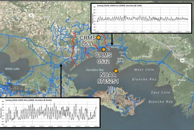
The Four Closure model was validated using three gage locations which collected water level and salinity data. One NOAA gage is located at Cypremort Point and two Coastwide Reference Monitoring System (CRMS) gages are located in Vermilion Bay and near Delcambre-Avery Canal. Gage locations are shown in Figure 4-4, and Table 4-1 lists the gage attributes.
Water level and salinity outputs from the Four Closure model compare favorably with observed gage data. Figures 4-5 through 4-10 compare observed water levels and salinity to the Four Closure model outputs. During January and February of 2010, the Four Closure model showed bi-directional discharge in the GIWW typically flowing to the east as it runs along Vermilion Bay (yellow arrows in Figure 4-4).
Table 4-1: Gage Attributes
Station Latitude Longitude Location
CRMS-0531 29°51’22” 91°58’42” Marsh CRMS-0532 29°49’30” 91°56’55” Channel NOAA-8765251 29°42.8’ 91°52.8’ Open Water
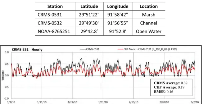
Figure 4-5: CRMS-531 Hourly Water Surface Elevation Validation
Figure 4-6: CRMS-531 Daily Salinity Validation
Figure 4-7: CRMS-532 Hourly Water Surface Elevation Validation
CRMS Average: 0.32 CHF Average: 0.19 RMSE: 0.16 CRMS Average: 0.79 CHF Average: 1.36 RMSE: 0.36 CRMS Average: 0.18 CHF Average: 0.29 RMSE: 0.18
Figure 4-8: CRMS-532 Daily Salinity Validation
Figure 4-9: NOAA 8765251 Hourly Water Surface Elevation Validation
Figure 4-10: NOAA 8765251 Daily Salinity Validation
CRMS Average: 0.49 CHF Average: 2.12 RMSE: 0.74 CRMS Average: 0.06 CHF Average: 0.29 RMSE: 0.27 CRMS Average: 0.38 CHF Average: 1.86 RMSE: 0.64
5.0
RESULTS
Several scenarios were analyzed to determine water level and salinity impacts due to closure structure placement. Four scenarios were analyzed with Inland closure structures or closure structures south of the GIWW (Figure 5-1). The southern structures were placed across Vermilion River, Boston Canal, Oaks Canal, Delcambre-Avery Canal, and Weeks Bay. The inland structures were placed across Delcambre-Avery Canal and Bayou Tigre.
• Scenario 1: South Structures (shown in yellow in Figure 5-1) with 2010 Tides and 2010 Channel Discharges
• Scenario 2: South Structures with 2010 Tides, 2010 Channel Discharges, and Large
Atchafalaya River Discharge
• Scenario 3: South Structures with 2010 Tides, 2010 Channel Discharges, and 50-year
Rainfall Event
• Scenario 4: Inland Structures (shown in orange in Figure 5-1) with 2010 Tides, 2010 Channel Discharges, and 50-year Rainfall Event
5.1
Scenario 1: South Structures with 2010 Tides and 2010
ChannelDischarges
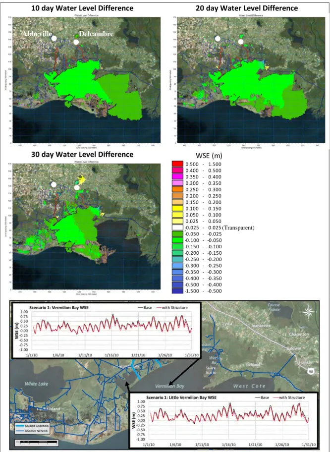
Scenario 1 examined the impacts of closure structures placed south of the GIWW with tides and channel discharges from 2010. The purpose of this scenario was to determine if placement of the closure structures would impact salinity transport in the Vermilion Bay vicinity. Figures 5-2
through 5-4 compare discharge, water level, and salinity at hourly and ten day increments through January 2010. The yellow and green values shown in Figures 5-2 and 5-3 are areas of minimal impact.
The addition of closure structures tended to damp discharge variability along the GIWW and increase the bi-directional discharge to the east. The water levels showed minimal impacts due to closure structures south of the GIWW, but there was a slight shift in the tidal cycle. Salinities increased in Vermilion Bay due to freshwater routed through the GIWW around Vermilion Bay. The water level impacts do not appear substantial enough to affect the Vermilion Bay ecosystem. Salinity levels increase over time and would require further analysis to determine ecosystem impacts if this scenario was selected for storm surge reduction benefits.
10 day Water Level Difference 20 day Water Level Difference
30 day Water Level Difference
Figure 5-3: Scenario 1 Water Level Comparison
0.500 - 1.500 0.400 - 0.500 0.350 - 0.400 0.300 - 0.350 0.250 - 0.300 0.200 - 0.250 0.150 - 0.200 0.100 - 0.150 0.050 - 0.100 0.025 - 0.050 -0.025 - 0.025 -0.050 - -0.025 -0.100 - -0.050 -0.150 - -0.100 -0.200 - -0.150 -0.250 - -0.200 -0.300 - -0.250 -0.350 - -0.300 -0.400 - -0.350 -0.500 - -0.400 -1.500 - -0.500 WSE (m) (Transparent) Abbeville Delcambre
10 day Salinity Difference 20 day Salinity Difference
30 day Salinity Difference
Figure 5-4: Scenario 1 Salinity Comparison
2.0 - 4.0 1.6 - 2.0 1.4 - 1.6 1.2 - 1.4 1.0 - 1.2 0.8 - 1.0 0.6 - 0.8 0.4 - 0.6 0.2 - 0.4 0.1 - 0.2 -0.1 - 0.1 -0.2 - -0.1 -0.4 - -0.2 -0.6 - -0.4 -0.8 - -0.6 -1.0 - -0.8 -1.2 - -1.0 -1.4 - -1.2 -1.6 - -1.4 -2.0 - -1.6 -4.0 - -2.0 Salinity (ppt) (Transparent) Abbeville Delcambre
5.2
Scenario 2: South Structures with 2010 Tides, 2010
ChannelDischarges, and Large
Atchafalaya Discharge
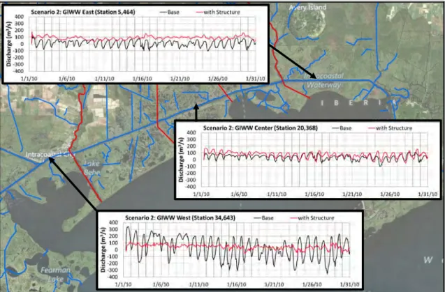
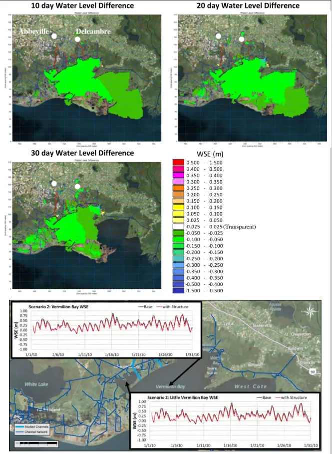
Scenario 2 examined the impacts of closure structures placed south of the GIWW with tides and channel discharges from 2010, but introduced high freshwater discharge from Atchafalaya River and Wax Lake Outlet during the flood of 2011 (see Appendix A for discharge data). The purpose of this scenario was to examine how the structures would impact salinity with abnormally high levels of freshwater inflow from the east. The majority Atchafalaya River and Wax Lake discharge exits the GIWW before reaching the project area. The bi-directional discharge in the GIWW tended to the east with the increased discharge from Wax Lake Outlet and the Atchafalaya River. Figures 5-5 through 5-7 compare discharge, water level, and salinity at hourly and ten day increments for January 2010 (yellow and green values are areas of minimal impact). The results for Scenario 2 are similar to Scenario 1: damped GIWW discharge, minimal impacts to water levels, and increased Vermilion Bay salinity. Further analysis of long term salinities and discharges would be required is if this scenario was selected for storm surge reduction benefits.
10 day Water Level Difference 20 day Water Level Difference
30 day Water Level Difference
Figure 5-6: Scenario 2 Water Level Comparison
0.500 - 1.500 0.400 - 0.500 0.350 - 0.400 0.300 - 0.350 0.250 - 0.300 0.200 - 0.250 0.150 - 0.200 0.100 - 0.150 0.050 - 0.100 0.025 - 0.050 -0.025 - 0.025 -0.050 - -0.025 -0.100 - -0.050 -0.150 - -0.100 -0.200 - -0.150 -0.250 - -0.200 -0.300 - -0.250 -0.350 - -0.300 -0.400 - -0.350 -0.500 - -0.400 -1.500 - -0.500 WSE (m) (Transparent) Abbeville Delcambre
10 day Salinity Difference 20 day Salinity Difference
30 day Salinity Difference
Figure 5-7: Scenario 2 Salinity Comparison
2.0 - 4.0 1.6 - 2.0 1.4 - 1.6 1.2 - 1.4 1.0 - 1.2 0.8 - 1.0 0.6 - 0.8 0.4 - 0.6 0.2 - 0.4 0.1 - 0.2 -0.1 - 0.1 -0.2 - -0.1 -0.4 - -0.2 -0.6 - -0.4 -0.8 - -0.6 -1.0 - -0.8 -1.2 - -1.0 -1.4 - -1.2 -1.6 - -1.4 -2.0 - -1.6 -4.0 - -2.0 Salinity (ppt) (Transparent) Abbeville Delcambre
5.3
Scenario 3: South Structures with 2010 Tides, 2010 Channel Discharges, and
50-year Rainfall Event
Scenario 3 analyzed the impacts of closure structures south of the GIWW during a 50-year, 24-hour rainfall event with tides and channel discharges from 2010. The purpose of this scenario was to examine water level impacts and salinity impacts during a large rainfall event. The 50-year, 24-hour rainfall event was applied uniformly over the model domain. As shown in Figures 5-8 through 5-12, the closure structures damped GIWW discharge, caused localized ponding, slightly decreased Vermilion Bay water levels, and increased Vermilion Bay salinity. The yellow and green values shown in Figures 5-9 and 5-10 are areas of minimal impact.
Placement of the closure structures during a 50-year, 24-hour rainfall event increased easterly discharge along the GIWW. Figure 5-11 shows the maximum water levels over the 15 day period. Ponding due to the closure structures is most pronounced around Delcambre-Avery Canal and the Weeks Bay closure structure. Similar to the other scenarios, Scenario 3 increased salinity in Vermilion Bay (Figure 5-12).
3 day Water Level Difference 6 day Water Level Difference
9 day Water Level Difference
Figure 5-9: Scenario 3 Water Level Comparison
0.500 - 1.500 0.400 - 0.500 0.350 - 0.400 0.300 - 0.350 0.250 - 0.300 0.200 - 0.250 0.150 - 0.200 0.100 - 0.150 0.050 - 0.100 0.025 - 0.050 -0.025 - 0.025 -0.050 - -0.025 -0.100 - -0.050 -0.150 - -0.100 -0.200 - -0.150 -0.250 - -0.200 -0.300 - -0.250 -0.350 - -0.300 -0.400 - -0.350 -0.500 - -0.400 -1.500 - -0.500 WSE (m) (Transparent) Abbeville Delcambre
3 day Salinity Difference 6 day Salinity Difference
9 day Salinity Difference
Figure 5-10: Scenario 3 Salinity Comparison
2.0 - 4.0 1.6 - 2.0 1.4 - 1.6 1.2 - 1.4 1.0 - 1.2 0.8 - 1.0 0.6 - 0.8 0.4 - 0.6 0.2 - 0.4 0.1 - 0.2 -0.1 - 0.1 -0.2 - -0.1 -0.4 - -0.2 -0.6 - -0.4 -0.8 - -0.6 -1.0 - -0.8 -1.2 - -1.0 -1.4 - -1.2 -1.6 - -1.4 -2.0 - -1.6 -4.0 - -2.0 Salinity (ppt) (Transparent) Abbeville Delcambre
Figure 5-11: Scenario 3 Maximum Water Level Comparison over 15 Days 0.500 - 1.500 0.400 - 0.500 0.350 - 0.400 0.300 - 0.350 0.250 - 0.300 0.200 - 0.250 0.150 - 0.200 0.100 - 0.150 0.050 - 0.100 0.025 - 0.050 -0.025 - 0.025 -0.050 - -0.025 -0.100 - -0.050 -0.150 - -0.100 -0.200 - -0.150 -0.250 - -0.200 -0.300 - -0.250 -0.350 - -0.300 -0.400 - -0.350 -0.500 - -0.400 -1.500 - -0.500 WSE (m) 2.0 - 4.0 1.6 - 2.0 1.4 - 1.6 1.2 - 1.4 1.0 - 1.2 0.8 - 1.0 0.6 - 0.8 0.4 - 0.6 0.2 - 0.4 0.1 - 0.2 -0.1 - 0.1 -0.2 - -0.1 -0.4 - -0.2 -0.6 - -0.4 -0.8 - -0.6 -1.0 - -0.8 -1.2 - -1.0 -1.4 - -1.2 -1.6 - -1.4 -2.0 - -1.6 -4.0 - -2.0 Salinity (ppt) Abbeville Delcambre Abbeville Delcambre
5.4
Scenario 4: Inland Structures with 2010 Tides,
ChannelDischarges, and 50-year
Rainfall Event
Scenario 4 analyzed the impacts of inland closure structures at Delcambre-Avery Canal and Bayou Tigre during a 50-year, 24-hour rainfall event with tides and channel discharges from 2010 (Figure 5-13). The purpose of this scenario was to examine water level and ponding impacts due to inland structure placement during a large rainfall event. Salinity was not examined. Scenario 4 was examined over 15 days which would be an abnormally long duration for the structures to be closed.
Minimal water level impacts were seen in Vermilion Bay; however, the closure structures caused ponding along Delcambre-Avery Canal and Tigre Bayou (Figure 5-14). Figure 5-15 shows maximum water levels over the 15 day period. Pump stations could be used to minimize ponding. Bayou Tigre would require a pump station with a 15 m3/s capacity and
Delcambre-Avery Canal would require an 8 m3/s capacity pump station to relieve upstream ponding due to
closure structures.
3 day Water Level Difference 6 day Water Level Difference
9 day Water Level Difference
Figure 5-14: Scenario 4 Water Level Comparison
0.500 - 1.500 0.400 - 0.500 0.350 - 0.400 0.300 - 0.350 0.250 - 0.300 0.200 - 0.250 0.150 - 0.200 0.100 - 0.150 0.050 - 0.100 0.025 - 0.050 -0.025 - 0.025 -0.050 - -0.025 -0.100 - -0.050 -0.150 - -0.100 -0.200 - -0.150 -0.250 - -0.200 -0.300 - -0.250 -0.350 - -0.300 -0.400 - -0.350 -0.500 - -0.400 -1.500 - -0.500 WSE (m) Abbeville Delcambre
Figure 5-15: Scenario 4 Maximum Water Level Comparison over 15 Days
6.0
DISCUSSION AND CONCLUSION
After examining the results from the Four Closure Structures model in the Vermilion Bay area, the modeling team found that Scenarios 1 and 2 showed little impact to water levels, while Scenarios 3 and 4 showed larger impacts. Scenarios 1, 2, and 3 showed impacts to salinity, while salinity was not examined in Scenario 4.
Structures south of the GIWW in Scenarios 1, 2, and 3 typically had little impact on water levels in Vermilion bay while increasing salinity. The increase in Vermilion Bay salinity under these scenarios is largely due to freshwater riverine inputs being rerouted through the GIWW and not entering the northern portions of Vermilion Bay. Due to the closure of the four canals and Weeks bay, the freshwater is re-routed and lowered the salinity levels in West Cote Blanche Bay. The inland closure structures in Scenario 4 caused large areas of ponding near Delcambre, Louisiana. Runoff from the 50-year, 24-hour storm event began to pond as it reached the
0.500 - 1.500 0.400 - 0.500 0.350 - 0.400 0.300 - 0.350 0.250 - 0.300 0.200 - 0.250 0.150 - 0.200 0.100 - 0.150 0.050 - 0.100 0.025 - 0.050 -0.025 - 0.025 -0.050 - -0.025 -0.100 - -0.050 -0.150 - -0.100 -0.200 - -0.150 -0.250 - -0.200 -0.300 - -0.250 -0.350 - -0.300 -0.400 - -0.350 -0.500 - -0.400 -1.500 - -0.500 WSE (m) Abbeville Delcambre
closure structures along Delcambre-Avery Canal and Bayou Tigre. This area did not have enough hydraulic connections to allow for adequate drainage of the area with these two large channels closed.
7.0
REFERENCES
Meselhe, Ehab A. and Robert L. Miller. 2007. Hydrologic Modeling and Budget Analysis of the Southwestern Louisiana Chenier Plain. Louisiana Coastal Area Science and Technology Program Office.
USGS. 2003. Surface-Water Hydrology of the Gulf Intracoastal Waterway in South-Central Louisiana, 1996-1999. United States Geological Survey.
APPENDIX A: Model Input Data
Figure A-1: Daily Rainfall
Figure A-2: 50-year, 24-hour Storm Event Rainfall
Figure A-3: Freshwater Bayou Lock Schedule (2010)
Figure A-4: Freshwater Bayou Lock Schedule (January – March 2010)
Figure A-5: Schooner Bayou Lock Schedule (2010)
Figure A-7: Atchafalaya River Discharge (January – March 2010 and 2011)
Figure A-8: Wax Lake Outlet Discharge (January – March 2010 and 2011)
Figure A-10: Daily Rainfall Evapotranspiration (January – March 2010)
APPENDIX B: Water Surface Elevation and Salinity Comparisons
0-10 day Average Water Level Difference 0-10 day Average Salinity Difference
10-20 day Average Water Level Difference 10-20 day Average Salinity Difference
20-30 day Average Water Level Difference 20-30 day Average Salinity Difference
0-10 day Average Water Level Difference 0-10 day Average Salinity Difference
10-20 day Average Water Level Difference 10-20 day Average Salinity Difference
20-30 day Average Water Level Difference 20-30 day Average Salinity Difference
0-10 day Average Water Level Difference 0-10 day Average Salinity Difference
10-20 day Average Water Level Difference 10-20 day Average Salinity Difference
20-30 day Average Water Level Difference 20-30 day Average Salinity Difference
0-10 day Average Water Level Difference
10-20 day Average Water Level Difference
20-30 day Average Water Level Difference
APPENDIX C: MIKE FLOOD Solver Routines
The following MIKE FLOOD explanation was copied directly from Meselhe and Miller 2007:
Numerical Modeling with MIKE FLOOD
MIKE FLOOD by the Danish Hydraulic Institute (DHI) is the modeling software used to simulate the Chenier Plain hydrodynamics. MIKE FLOOD is a commercially-available robust hydrodynamic and advection-dispersion modeling package linking a one-dimensional channel network with a two-dimensional relief grid (Its capability of handling a tidally-driven estuarine system such as the coastal Chenier Plain, and its GIS-based interface, makes it suitable in the present case). Given the proper inputs from the tides, upstream discharge, wind, and bathymetry, the model is capable of capturing the hydrodynamics of the system quite well. In addition, the inclusion of structures, wetting and drying capabilities, and the modeling of lateral outflow from the channels into the surrounding marshes make MIKE FLOOD an attractive modeling option.
MIKE FLOOD connects the channel network with the surrounding marsh and open water bodies (Figure B.1). This allows the modeler to represent the small-scale channel details and the floodplain flow separately. This in turn gives the modeler the ability to use a larger grid spacing (hence faster simulations compared to a grid-only representation) without omitting the structures, narrow cross-sections, and other small features affecting the circulation patterns.
Figure B-1: Overview of the Chenier Plain Modeling Scheme
MIKE11 is a hydraulic modeling software package that solves the equations of conservation of mass and momentum integrated over the cross section. Collectively, these equations are termed the “Saint-Venant” equations, and are derived on the basis of the following assumptions:
• The water is incompressible and homogeneous, i.e. without significant variations in density;
• The channel bottom slope is small (normal depth is greater than the critical depth);
• The wavelengths are large compared to the water depth. This ensures that the flow everywhere can be regarded as having a direction parallel to the bottom, i.e. vertical acceleration can be neglected and a hydrostatic pressure distribution along the vertical can be assumed; and
•The flow is subcritical.
The continuity and momentum-conservation equations are as follows: 𝜕𝑄 𝜕𝑥 + 𝜕𝐴 𝜕𝑡 =𝑞 [B.1] 𝜕𝑄 𝜕𝑡 + 𝜕 �𝛼 𝑄𝐴 �2 𝜕𝑥 +𝑔𝐴 𝜕ℎ 𝜕𝑥+ 𝑔𝑄|𝑄| 𝐶2𝐴𝑅 = 0 [B.2] where, Q = discharge, A = flow area, q = lateral inflow,
h = stage above datum,
C = Chezy resistance coefficient,
R = hydraulic or resistance radius, and
α = momentum distribution coefficient.
The Saint-Venant equations in MIKE11 are handled by the method of finite differences using the 6-Point Abbott Scheme after the founder of MIKE11, Mike Abbott. For more information, the interested reader is referred to the MIKE11 Reference Manual (2004 Ed.).
Model stability depends on the spacing of grid points (Q and h), cross-section inverts, and the time step. Generally, increasing the number of points with a decreasing time step improves the stability of the simulation. This stability criterion is represented by a Courant number condition.
𝑉∆𝑡
∆𝑥 ≤1 𝑡𝑜 2 [B.4]
Here Cr is the Courant Number, Δt is the time step, V represents the cross-sectional velocity, y is the water depth, g is the gravitational acceleration, and Δx is the spacing between two grid points.
MIKE11 Advection-Dispersion Module
MIKE11 solves the vertically-integrated equations of mass conservation and transport of a dissolved constituent. The solutions obtained will describe the movement of the salinity in the Chenier Plain. The one-dimensional equation for conservation of mass of a constituent in solution (such as temperature, salinity, etc) can be expressed as follows:
𝜕𝐴𝐶 𝜕𝑡 + 𝜕𝑄𝐶 𝜕𝑥 − 𝜕 𝜕𝑥 �𝐴𝐷 𝜕𝐶 𝜕𝑥�=−𝐴𝐾𝐶+𝐶2𝑞 [B.5]
Here, C is concentration (arbitrary unit), D is the dispersion coefficient, K is a linear decay coefficient, q is the lateral inflow, and C2 is source/sink concentration. The dispersion coefficient is related to the cross sectional average velocity via the following relationship:
𝐷=𝑎𝑉𝑏 [B.6]
where a and b are constants to be specified and they can be considered as additional calibration parameters. More information about the solution schemes and detailed descriptions of the various parameters are available in the MIKE11 DHI Software Reference Manual (2004 Ed.).
MIKE21 Hydrodynamic Module
The hydrodynamic model in the MIKE21 Flow Model (MIKE21 HD) is a general modeling system for the simulation of water levels and flows in estuaries, bays, and coastal areas. It simulates time-varying two-dimensional flows in one layer (vertically homogeneous) fluids and has been used in a large number of studies. The following depth-integrated equations of mass and momentum conservation describe the flow and water level variation.
𝜕𝜍 𝜕𝑡+ 𝜕𝑝 𝜕𝑥+ 𝜕𝑞 𝜕𝑦= 𝜕𝑑 𝜕𝑡 [B.7] 𝜕𝑝 𝜕𝑡+ 𝜕 𝜕𝑥 � 𝑝2 ℎ �+ 𝜕 𝜕𝑦 � 𝑝𝑞 ℎ �+𝑔ℎ 𝜕𝜁 𝜕𝑥+𝑔𝑝�𝑝 2+𝑞2 𝐶2ℎ2 1 𝜌𝑤� 𝜕 𝜕𝑥(ℎ𝜏𝑥𝑥) + 𝜕 𝜕𝑦 �ℎ𝜏𝑥𝑦�� − Ω𝑞− 𝑓(𝑉)𝑉𝑥+𝜌𝑤ℎ𝜕𝑥𝜕(𝑝𝑎) = 0 [B.8]
𝜕𝑝 𝜕𝑡+ 𝜕 𝜕𝑦 � 𝑞2 ℎ �+ 𝜕 𝜕𝑥 � 𝑝𝑞 ℎ �+𝑔ℎ 𝜕𝜁 𝜕𝑡+ 𝑔𝑞�𝑝2+𝑞2 𝐶2ℎ2 1 𝜌𝑤� 𝜕 𝜕𝑦 �ℎ𝜏𝑦𝑦�+𝜕𝑥 �ℎ𝜏𝜕 𝑥𝑦�� − Ω𝑝− 𝑓(𝑉)𝑉𝑦+𝜌𝑤ℎ𝜕𝑥𝑦𝜕 (𝑝𝑎) = 0 [B.9] where,
h(x,y,t) = the water depth (ζ-d) in m,
d(x,y,t) = the time-varying water depth in m; ζ(x,y,t) = the surface elevation in m;
p and q(x,y,t) = flux densities in the x and y-directions in m3/s/m;
u and v = depth-averaged velocities in the x and y-directions in m/s;
C(x,y) = the Chezy resistance in m1/2/s;
g = the acceleration due to gravity in m/s2;
f(V) = the wind friction factor;
V, Vx, Vy(x,y,t) = wind speed and components in the x and y-directions in m/s; Ω(x,y) = the latitude-dependent Coriolis parameter in units s-1;
pa(x,y,t) = the atmospheric pressure in kg/m-s2; ρa = the density of water in kg/m3;
x and y = the space coordinates in m;
t = the time in s; and
τ, τxx, and τyy = the components of effective shear stress in N/m2.
MIKE21 HD makes use of a so-called Alternating Direction Implicit (ADI) technique to integrate the equations for mass and momentum conservation in the space-time domain. More information is available in the DHI MIKE21 HD Software Scientific Documentation (2005 Ed.).
MIKE21 Advection-Dispersion Module
The Advection/Dispersion (AD) module simulates the spreading of dissolved substances subject to advection and dispersion processes in lakes, estuaries and coastal regions. Specifically, MIKE21 is used here to simulate the horizontal circulation of salinity in the near-shore Gulf of Mexico, and Chenier Plain lakes and marsh. Transport of a dissolved substance in MIKE21 is governed by the mass-conservation equation:
𝜕(ℎ𝑐) 𝜕𝑡 + 𝜕(𝑢ℎ𝑐) 𝜕𝑥 + 𝜕(𝑣ℎ𝑐) 𝜕𝑦 = 𝜕 𝜕𝑥 �ℎ𝐷𝑥 𝜕𝑐 𝜕𝑥�+ 𝜕 𝜕𝑦 �ℎ𝐷𝑦 𝜕𝑐 𝜕𝑦� − 𝐹 ∗ ℎ ∗ 𝑐+𝑆 [B.10] Here, c is the compound concentration (arbitrary units); u and v are the depth-averaged horizontal velocity components in the x and y directions (m/s); h is the water depth (m); Dx and Dy are the dispersion coefficients in x and y directions (m2/s); F is the linear decay coefficient (s-1); S=Q
s*(cs-c); Qs is the source/sink discharge m3/s/m2; and cs is the concentration of compound in the source/sink discharge Qs. Information on the velocities u and v are provided from the hydrodynamic module.
Dispersion coefficients represent the combined effect of differential advection and diffusion. The dispersion coefficient is an important salinity calibration parameter as it accounts for the effects of numerical diffusion and depth-integration on the transport equations. More details including a report entitled “An Explicit Scheme of Advection-Diffusion Modeling in Two Dimensions” are given in the DHI MIKE21 AD Software Scientific Documentation (2005 Ed.).
MIKE FLOOD Coupling Program
As stated previously, the MIKE FLOOD mass-preserving links connect the MIKE11 channel network with the MIKE21 grid (Figure B.2).
Figure B-2: Schematization of the MIKE FLOOD Standard Link
The hydrodynamic and advective-diffusive transport equations for standard links are as follows: 𝜕𝑄𝑛+1 2� 𝜕𝑡 =− �𝑔𝐴 𝜕𝐻𝑛 𝜕𝑥 + 𝑄𝑛|𝑄𝑛| 𝐴 ∗ 𝐶2∗ 𝑅� [B.11]
Here, Q represents the flow rate (m3/s); A is the cross-sectional area (m2); x is the length in m; H
is the water depth in m; R represents the hydraulic radius in m; and C is the Chezy resistance (m1/2/s).
Concentrations of AD (salinity) components are transferred explicitly between MIKE11 and MIKE21 depending on the direction of the flow. For standard links with flow from MIKE11 and MIKE21, the concentration of the AD-component is imposed as with a standard MIKE21 source, i.e. as a flux of mass into the MIKE21 points:
∆ �𝜕𝑉 ∗ 𝐶𝑀21𝑛+1 2
�
𝜕𝑡 �=𝑄𝑛+1 2� ∗ 𝐶𝑀11𝑛 [B.12]
Here, C is concentration, V is the total volume in the linked cells, and Q represents the flow rate. When flow is going from MIKE21 to MIKE11, the modification to the AD-equation in MIKE21 is:
∆ �𝜕𝑉 ∗ 𝐶𝑀11𝑛+1 2
�
𝜕𝑡 �=𝑄𝑛+1 2� ∗ 𝐶𝑀21𝑛 [B.13]
In summary MIKE FLOOD simulates the exchange between channel and marsh with links and describes a channel connecting to an open water body. In this way the modeler can describe the fine details (dynamic structures, narrow cross-sections, abrupt changes in channel dimensions) with a 1D channel network, while simulating the floodplain and Gulf of Mexico flow fields with a 2D grid.