Audio Engineering Society
Convention Paper
Presented at the 111th Convention
2001 September 21–24
New York, NY, USA
This convention paper has been reproduced from the author's advance manuscript, without editing, corrections, or consideration by the Review Board. The AES takes no responsibility for the contents. Additional papers may be obtained by sending request and remittance to Audio Engineering Society, 60 East 42nd Street, New York, New York 10165-2520, USA; also see www.aes.org. All rights reserved. Reproduction of this paper, or any portion thereof, is not permitted without direct permission from the
Journal of the Audio Engineering Society.
___________________________________
Wavefront Sculpture Technology
MARCEL URBAN, CHRISTIAN HEIL, PAUL BAUMAN
L-ACOUSTICS
Gometz-La-Ville, 91400 France
ABSTRACT
We introduce Fresnel’s ideas in optics to the field of acoustics. Fresnel analysis provides an effective, intuitive approach to the understanding of complex interference phenomena and thus opens the road to establishing the criteria for the effective coupling of sound sources and for the coverage of a given audience geometry in sound reinforcement applications. The derived criteria form the basis of what is termed Wavefront Sculpture Technology.
0 INTRODUCTION
This paper is a continuation of the preprint presented at the 92nd AES Convention in 1992 [1]. Revisiting the conclusions of this article, which were based on detailed mathematical analysis and numerical methods, we now present a more qualitative approach based on Fresnel analysis that enables a better understanding of the physical phenomena involved in arraying discrete sound sources. From this analysis, we establish criteria that define how an array of discrete sound sources can be assembled to create a continuous line source. Considering a flat array, these criteria turn out to be the same as those which were originally developed in [1]. We also consider a variable curvature line source and define other criteria required to produce a wave field that is free of destructive interference over a predefined coverage region for the array, as well as a wave field intensity that decreases as the inverse of the distance over the audience area. These collective criteria are termed Wavefront Sculpture Technology1 (WST) Criteria.
1 MULTIPLE SOUND SOURCE RADIATION - A REVIEW
The need for more sound power to cover large audience areas in sound reinforcement applications implies the use of more and more sound sources. A common practice is to configure many loudspeakers in arrays or clusters in order to achieve the required
1 Wavefront Sculpture Technology and WST are trademarks of
L-ACOUSTICS
sound pressure level (SPL). While an SPL polar plot can characterize a single loudspeaker, an array of multiple loudspeakers is not so simple. Typically, trapezoidal horn-loaded loudspeakers are assembled in fan-shaped arrays according to the angles determined by the nominal horizontal and vertical coverage angles of each enclosure in an attempt to reduce overlapping zones that cause destructive interference. However, since the directivity of the individual loudspeakers varies with frequency, the sound waves radiated by the arrayed loudspeakers do not couple coherently, resulting in interference that changes with both frequency and listener position.
Considering early line array systems (column speakers), apart from narrowing of the vertical directivity, another problem is the appearance of secondary lobes outside the main beamwidth whose SPL can be as high as the on-axis level. This can be improved with various tapering or shading schemes, for example, Bessel weighting. The main drawback is a reduced SPL and, for the case of Bessel weighting, it was shown that the optimum number of sources was five [2]. This is far from being enough for open-air performances.
In [1] we advocated the solution of a line source array to produce a wave front that is as continuous as possible. Considering first a flat, continuous and isophasic (constant phase) line source, we demonstrated that the sound field exhibits two spatially distinct regions: the near field and the far field. In the near field, wave
fronts propagate with 3 dB attenuation per doubling of distance (cylindrical wave propagation) whereas in the far field there is 6 dB attenuation per doubling of distance (spherical wave propagation). It is to be noted that usual concepts of directivity, polar diagrams and lobes only make sense in the far field (this is developed in appendix 1).
Considering next a line source with discontinuities, we also described a progressively chaotic behavior of the sound field as these discontinuities become progressively larger. This was confirmed in 1997 [3] when Smith, working on an array of 23 loudspeakers, discovered that 7 dB SPL variations over 1 foot was a common feature in the near field. Smith tried raised cosine weighting approaches in order to diminish this chaotic SPL and was somewhat successful, but it is not possible to have, at the same time, raised cosine weighting for the near field and Bessel weighting for the far field. In [1] we showed that a way to minimize these effects is to build a quasi-continuous wave front. The location of the border between the near field and the far field is a key parameter that describes the wave field. Let us call dB the
distance from the array to this border. We will make the approximation that if F is the frequency in kHz then λ=1/(3F) where λ is the wavelength in metres. Considering a flat, continuous line source of height H that is radiating a flat isophasic wavefront, we demonstrated in [1] that a reasonable average of the different possible expressions for dB obtained using either geometric,
numerical or Fresnel calculations is:
(
FH
)
H
F
d
B3
1
1
2
3
2 2−
=
where dB and H are in meters, F is in kHz.
There are three things to note about this formula:
1) The root factor indicates that there is no near field for frequencies lower than 1/(3H). Hence a 4 m high array will radiate immediately in the far field mode for frequencies less than 80 Hz. 2) For frequencies above 1/(3H) the near field extension is almost linear with frequency.
3) The dependence on the dimension H of the array is not linear but quadratic.
All of this indicates that the near field can extend quite far away. For example, a 5.4 m high flat line source array will have a near field extending as far as 88 meters at 2 kHz.
We also demonstrated in [1] that a line array of sources, each of them radiating a flat isophase wave front, will produce secondary lobes not greater than –12 dB with respect to the main lobe in the far field and SPL variations not greater than ± 3 dB within the near field region, provided that:
♦ Either the sum of the flat, individual radiating areas covers more than 80% of the vertical frame of the array, i.e., the target radiating area
♦ Or the spacing between the individual sound sources is
smaller than 1/(6F) , i.e., λ/2.
These two requirements form the basis of WST Criteria which, in turn, define conditions for the effective coupling of multiple sound sources. In the following sections, we will derive these results using the Fresnel approach along with further results that are useful for line source acoustical predictions.
Figure 1 displays a cut view of the radiated sound field. The SPL is significant only in the dotted zone (ABCD + cone beyond BC). A more detailed description is deferred to Section 4.
Figure 1:
Radiated SPL of a line source AD of height H. In the near field, the SPL decreases as 3 dB per doubling of distance, whereas in the far field, the SPL decreases as 6 dB per doubling of distance.
It should be noted that different authors have come up with various expressions for the border distance:
dB = 3H Smith [3]
dB = H/π Rathe [4]
dB = maximum of (H , λ/6) Beranek [5]
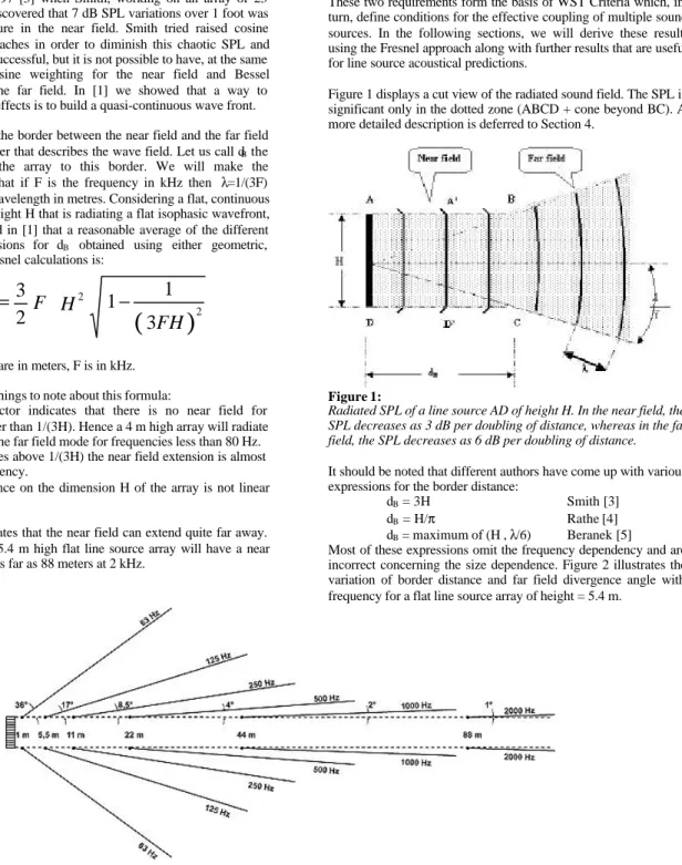
Most of these expressions omit the frequency dependency and are incorrect concerning the size dependence. Figure 2 illustrates the variation of border distance and far field divergence angle with frequency for a flat line source array of height = 5.4 m.
Figure 2:
Representation of the variation of border distance and far field divergence angle with frequency for a flat line source array of height 5.4 metres.
2 THE FRESNEL APPROACH FOR A CONTINUOUS LINE SOURCE
The fact that light is a wave implies interference phenomena when an isophasic and extended light source is looked at from a given point of view. These interference patterns are not easy to predict but Fresnel, in 1819, described a way to semi-quantitatively picture these patterns. Fresnel's idea was to partition the main light source into fictitious zones made up of elementary light sources. The zones are classified according to their arrival time differences to the observer in such a way that the first zone appears in phase to the observer (within a fraction of the wave length λ). The next zone consists of elementary sources that are in-phase at the observer position, but are collectively in phase opposition with respect to the first zone, and so on. A more precise analysis shows that the fraction of wave length is λ/2 for a 2-dimensional source and λ/2.7 for a 1-dimensional source (please see appendix 2 for further details).
We will apply Fresnel’s concepts to the sound field of extended sources. Let us consider first a perfectly flat, continuous and isophasic line source. To determine how this continuous wave front will perform with respect to a given listener position, we draw spheres centered on the listener position whose radii are incremented by steps of λ/2 (see figures 3 and 4). The first radius equals the tangential distance that separates the line source and the listener. Basically two cases can be observed:
1. A dominant zone appears:
The outer zones are alternatively in-phase and out-of-phase. Their size is approximately equal and they cancel each other out. We can then consider only the largest, dominant zone and neglect all others. We assume that this dominant zone is representative of the SPL radiated by the line source. This is illustrated in Figure 3 where it is seen that for an observer facing the line source the sound intensity corresponds roughly to the sound radiated by the first zone.
2. No dominant zone appears in the pattern and almost no sound is radiated to the observer position. Referring to figure 4, this illustrates the case for an off-axis observer.
Figure 3:
Observer facing the line source. On the right part (side view), circles are drawn centered on the observer O, with radii increasing by steps of λ/2. The pattern of intersections on the source AB is shown on the left part (front view). These define the Fresnel zones.
Figure 4:
The observer O, is no longer facing the line source. The corresponding Fresnel zones are shown on the left part (front view). There is no dominant zone and individual zones cancel each other off-axis.
Moving the observation point to a few locations around the line source and repeating the exercise, we can get a good qualitative picture of the sound field radiated by the line source at a given frequency.
Note that the Fresnel representations of figures 3 and 4 are at a single frequency. The effects of changing frequency and the on-axis listener position are shown in Figure 5.
Figure 5:
The effect of changing frequency and listener position.
As the frequency is decreased, the size of the Fresnel zone grows so that a larger portion of the line source is located within the first dominant zone. Conversely, as the frequency increases, a reduced portion of the line source is located inside the first dominant zone. If the frequency is held constant and the listener position is closer to the array, less of the line source is located within the first dominant zone due to the increased curvature. As we move further away, the entire line source falls within the first dominant zone.
3 EFFECTS OF DISCONTINUITIES ON LINE SOURCE ARRAYS
In the real world, a line source array results from the vertical assembly of separate loudspeaker enclosures. The radiating transducers do not touch each other because of the enclosure wall thicknesses. Assuming that each transducer originally radiates a flat wave front, the line source array is no longer continuous. In this section, our goal is to analyze the differences versus a
continuous line source in order to define acceptable limits for a line source array.
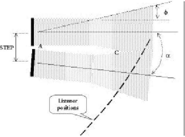
Let us consider a collection of flat isophasic line sources of height D, with their centers spaced by STEP. To understand the sound field radiated by this array, we replace the real array by the coherent sum of two virtual sources as displayed in figure 6. The real array is equivalent to the sum of a continuous line source and a disruption grid which is in phase opposition with this perfect continuous source.
Figure 6:
The left part shows a real array consisting of sources of size D spaced apart by STEP. The right part shows two virtual sources considered as a perturbation and a continuous ideal source. Their sum is equivalent to the real array.
3.1 Angular SPL of the Disruption Grid
The pressure magnitude produced by the disruption grid is proportional to the thickness of the walls of the loudspeaker enclosures. Figure 7 illustrates how to predict the effect of the disruption grid in particular directions at a given frequency. The complex addition of the virtual sound sources of the grid creates an interference pattern that cannot be neglected, unless by reducing their size.
Figure 7:
When the observer position is very far, Fresnel circles are transformed into segments. The left figure shows that when observing at the angle θdip, half the sources are in phase opposition
with the other half thus producing a null pressure. On the right, it is seen that as we move further off-axis, all sources are in phase thus producing a strong pressure.
Let us perform Fresnel analysis for an observer at infinity. In this case, circles crossing the grid become straight lines. Now let us consider the interference pattern as a function of polar angle. In the forward direction (θ = 0), all sources appear in phase. At θdip, half
the sources are in phase and the other half are in phase opposition, thus they cancel each other and the resulting SPL is very small. At
θpeak, all sources are back in phase and produce an SPL as strong as
in the forward direction.
Therefore, the discontinuities in a line source generate secondary lobes outside the beamwidth whose effects are proportional to the size of the discontinuities. This is the first reason why it is desirable to attempt to approximate a continuous line source as closely as possible.
From this qualitative approach, we understand that secondary lobes appear in the sound field due to the grid effect. The angles where the secondary peak and the secondary dip arise are given by:
)
sin(
θ
peak=
λ
STEP
2
/
)
sin(
θ
dip=
λ
STEP
If the first notch appears at θdip > π/2, it will not be detrimental to
the radiated sound field. This translates to:
STEP
6
1
1
)
sin(
θ
dip
≥
⇒
F
≤
As before, F is in kHz and STEP is in meters. Alternatively, expressing STEP in terms of wavelength:
2
λ
≤
STEP
In other words, the maximum separation or STEP between individual sound sources must be less than λ/2 at the highest frequency of the operating bandwidth in order for the individual sound sources to properly couple without introducing strong off-axis lobes.
As an example, if STEP = 0.5m, notches will not appear in the sound field provided that F < 300 Hz. In the next section, we intend to quantify the disruption due to the walls of enclosures and to establish limits on the spacing between radiating transducers.
3.2 The Active Radiating Factor (ARF)
Now we have to do some math to determine the superposition of pressure. The pressure delivered by the ideal continuous source in the far field is:
θ
θ
sin
2
sin
2
sin
H
k
H
k
H
p
continuous
∝
The pressure of the disruption grid is:
)
sin
2
sin(
)
sin
2
)
1
sin((
)
(
θ
θ
STEP
k
STEP
k
N
D
STEP
p
disrupt+
−
−
∝
Where D is the active radiating height of an individual sound element as shown in Figure 6.
In the forward direction, i.e: θ = 0, we have:
H
p
continuous(
θ
=
0
)
∝
)
)(
1
(
)
0
(
N
STEP
D
p
disruptθ
=
∝
−
+
−
)
)(
1
(
N
STEP
D
H
p
p
p
real=
continuous+
disrupt∝
−
+
−
STEP
D
N
p
real(
θ
=
0
)
∝
(
+
1
)
−
At the secondary peak we have:
λ
θ
)
=
sin(
peakSTEP
π
λ
λ
π
θ
N
STEP
STEP
N
H
k
peak=
=
2
2
)
sin(
2
0
)
sin(
)
(
=
=
π
π
θ
N
N
H
p
continuous peak(
)
(
)
( )
0
(
N
1
)
(
STEP
D
)
p
p
p
disrupt peak disrupt peak real−
+
−
=
=
=
θ
θ
We now have to define an acceptable ratio for the height of a secondary lobe with respect to the main on-axis lobe. Based on the pattern of a perfect line source that produces secondary lobes in the far field not higher than –13.5 dB of the main lobe, it seems optimal to specify in our case a –13.5 dB ratio. Therefore we require:
4
.
22
1
)
0
(
2
)
(
2
≤
=
=
θ
θ
θ
p
p
real peak real[
]
22
.
4
1
)
1
(
)
)(
1
(
2
≤
−
+
−
+
−
STEP
D
N
D
STEP
N
73
.
4
1
1
1
1
≤
+
−
−
N
STEP
D
STEP
D
We define the Active Radiating Factor (ARF) as:
STEP
D
ARF
=
thus,)
)
1
(
73
.
4
1
1
(
82
.
0
+
+
≥
N
ARF
Therefore, when N is large, we find that ARF has to be larger than 82% if the secondary peak is to be 13.5 dB below the main forward peak. This confirms what was originally obtained in [1]. Note that a secondary peak of only 10dB below the main forward peak is obtained when ARF is equal to 76%. ARF is thus a factor which has to be carefully looked at.
When N is large, a practical formula relating ARF to the attenuation of the secondary side lobes in decibels, Atten(dB), is:
10
1
1
20 ) (dB AttenARF
−+
=
Note: Frequency dependency does not show up in the final formula for ARF. This is because we have assumed that the angle θpeak was
between 0 and π/2. However, it should be noted that if the frequency is low enough there will be no secondary peak and this is the only way that frequency dependency can enter into this calculation.
3.3 The First WST Criteria and Linear Arrays
Assuming that the line array consists of a collection of individual flat isophasic sources, we have just redefined the two criteria required in order to assimilate this assembly into the equivalent of a continuous line source as derived in [1]. These two conditions are termed Wavefront Sculpture Technology (WST) criteria:
♦ The sum of the individual flat radiating areas is greater than 80% of the array frame (target radiating area) or
♦ The frequency range of the operating bandwidth is limited to F<1/(6 STEP), i.e., the STEP distance between sources is less than λ/2.
Note: further WST criteria will be derived in the following sections.
For a slot whose width is small compared to its height D, ARF is D/STEP. For the case of touching circular sound sources, the average ARF is π/4 =75%. It is therefore impossible to satisfy the first criterion and for circular pistons the only way to avoid the secondary lobes is to specify that the maximum operating frequency be less than 1/(6D). In other words, the diameter of a circular piston has to be smaller than 1/(6F). While this is possible for frequencies lower than a few kHz it becomes impossible at higher frequencies. For example, at 16 kHz we would need touching pistons with diameters of a few millimeters.
From this example, we understand that there is a challenge as to how to fulfil the first criterion at higher frequencies.One solution might consist of arraying rectangular horns in such a way that their edges touch each other. However, an important consideration is that such devices do not radiate a flat isophasic wave front. Then, the next question to be answered becomes: how flat does the wave front have to be in order for the sources to couple correctly? Let us consider a collection of vertically arrayed horns, separated only by their edges. The radiated wave front exhibits ripples of magnitude s, as shown in figure 8. The most critical case occurs at high frequencies where the wavelength is becoming small, e.g., 2 cm at 16 kHz. According to Fresnel, when standing in the far field the radiated wavefront curvature (s), should not be greater than half the wavelength, i.e., 1 cm at 16 kHz. Unfortunately, the conditions are much more restrictive in the near field when considering high frequencies.
Figure 8:
This illustrates that vertically arraying conventional horns will not produce a flat wave front.
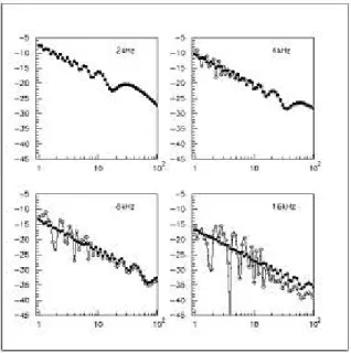
Figure 9 displays the calculated SPL versus distance for a line array of 30 horns, 0.15 m high, each of them producing a curved wave front of 0.3 m (ripple s = 10 mm). Comparison with a flat line source shows chaotic behavior of the line array, starting at 8 kHz and increasing with frequency. Apart from severe fluctuations in the SPL at higher frequencies, there is also a 4 dB loss at 16 kHz from 10 - 100 metres.
Figure 9:
SPL vs distance for a vertical array of 30 horns (total height = 4.5 m, wavefront curvature s=10 mm) calculated at 2, 4, 8 and 16 kHz. White dots: line array, black dots: continuous line source.
Another comparison displayed in figure 10 illustrates the cross section of the beam width which exhibits strong secondary peaks in the near field (20 m) at frequencies higher than 8 kHz.
Figure 10:
SPL along a vertical path, 20 m away from the vertical array of 30 horns (total height = 4.5 m, wavefront curvature s=10 mm) calculated at 2, 4, 8 and 16 kHz. White dots: line array, black dots: continuous line source.
It is therefore necessary to reduce wave front curvature by half (s < 5 mm), in order to create an “as good as” perfect line source up to 16 kHz. In effect, this will shift the sidelobe pattern observed in Figure 10 and the on-axis behaviour observed in Figure 9 from 8 kHz to 16 kHz. We conclude by stating that the deviation from a flat wave front should be less than λ/4 at the highest operating frequency (corresponding to 5 mm at 16 kHz).
For this reason, a waveguide has been specifically developed in order to generate a flat, isophasic wavefront at the exit of the device. The patented DOSC waveguide is incorporated in several commercially-available sound reinforcement systems that are designed to perform in accordance with WST criteria.
For the frequency range of 1.3 - 16 kHz, the sound pressure of a circular piston (i.e., the output of a compression driver) is passed through the waveguide where all possible acoustic path lengths are identical in length. This produces a wave front that is flat and isophasic (constant phase) at the rectangular aperture of the opening (see figure 11). This geometric transformation from circular to rectangular creates a wavefront that is sufficiently flat to satisfy the limits of acceptable curvature derived above and experiments have shown that wavefront curvature is less than 4 mm at 16 kHz. When multiple DOSC waveguides are vertically arrayed, this allows for satisfaction of the 80% ARF criterion provided that the angle between adjacent enclosures is less than 5 degrees (see section 6.2 for further details).
Figure 11:
WST Criteria Illustrated. On top we see the central portion of the DOSC waveguide that geometrically sets all possible sound path lengths to be identical from the circular entrance to the rectangular exit of the device, thus producing a flat, isophasic source for the high frequency section. The bottom figure shows a stack of 5 such devices (including the outer housing) which produces a vertical, flat sound source satisfying WST criteria 1.
4 SOUND FIELD RADIATED BY A FLAT LINE SOURCE ARRAY
4.1 Radiation as a Function of Distance
Considering a flat line source array, we want to understand why there is a near field (cylindrical wave propagation) and a far field (spherical wave propagation) and to derive an expression for the border distance. We will use Fresnel analysis to locate the border between the two regions (see [1] for analytical calculations). Let us consider a flat line source array of N discrete elements, operating at a given frequency. The observer is moving along the main axis of the radiation, as shown in figure 12. As the observer moves away from the line source, the number of sources in the dominant zone, Neff, increases until it reaches the maximum
number of available sources (h = H). Moving beyond this distance, the number of sources no longer varies.
Figure 12:
The first Fresnel zone height is h. This height grows as distance d increases until h = H. At greater distances, no more increase of the radiated power is expected.
Each source radiates a sound field as depicted in figure 1. We will place ourselves in the far field of each source (where spherical propagation applies). It will be detailed in section 6.2 that the condition that we are located in the far field of each element implies certain restrictions on the tilt angles between adjacent elements.
The total pressure magnitude is thus proportional to:
STEP
ARF
d
N
p
eff
∝
eff
while the SPL is proportional to the square of peff.
We need to know how Neff (or h) varies with the listener distance.
From figure 12, we calculate:
)
2
/
(
4
λ
+
λ
=
=
h
d
STEP
N
eff
For λ<<d, we have two simplified formulations for the SPL depending on the size of h:
When h < H:
ARF
Fd
ARF
d
h
I
I
I
nearfield flat nearfield flat 2 2 2 23
4
∝
⇒
∝
=
When h > HARF
d
H
I
I
farfield flat 2 2 2∝
=
We verify that as long as Neff < Nmax, the SPL decreases as 1/d,
defining the cylindrical wave propagation region. It is simple to extract the expression for border distance dB.
H
F
d
d
d
flat B flat B farfield flat flat B nearfield flatI
I
24
3
)
(
)
(
=
⇒
=
where dB and H are in meters, F is in kHz. The formula derived in
[1] for F>>1/3H, is 3/2 FH2, therefore Fresnel analysis predicts that the border distance is 50% closer.
When does a near field exist? With Fresnel we understood that as the distance of the listener decreases, the number of sources in the first zone decreases too, except for when λ/2 > H/2 because then the entire array is always in the first zone. Therefore, with Fresnel analysis, we have derived the same result as found in [1], i.e., there is no near field when F<1/(3H)
There is, however, the basic fact that even a continuous source displays ripples in the SPL of the near field, but with magnitude less than ± 3dB about the average.
This is the second reason for assigning ourselves the goal of producing a wave front as close as possible to a continuous sound source, i.e, in order to reduce ripples in the nearfield response. (recall that the first reason was in order to reduce sidelobe levels in the far field).
To illustrate this, the array studied in [3] consists of 23 dome tweeters with diameters of 25 mm. The STEP is 80 mm. The second criterion for arrayability is that the frequency be less than 1/(6STEP) = 1/(6*0.08) = 2 kHz. The first criterion is that for frequencies higher than 2 kHz, the ARF should be greater than 80%. Here the ARF is less than 25/80=30%. and we can conclude that above 2 kHz, this array will exhibit severe problems in the near field.
In figure 13, we compare the SPL of a continuous sound source 1.76 m high, with the array of 23 tweeters and calculate the SPL as a function of distance at 1 and 8 kHz. We see that below 2 kHz the continuous and discrete arrays are similar while for higher frequencies, the discrete array shows unacceptable SPL ripples over very small distances. We also plot the -3 dB (near field) and the -6 dB (far field) lines predicted from our analysis.
Figure 13:
SPL as a function of distance. Empty circles: 23 tweeters totaling a height of 1.76m. Full circles: a continuous array of the same height. The –3dB and the –6dB per doubling of distance lines are shown on the same figure to indicate the border between the near and far fields.
4.2 Vertical Pattern in the Far Field
With the help of Fresnel analysis, we now investigate the vertical directivity in the far field for a flat line array. The horizontal directivity is equivalent to that radiated by a single element. We saw previously in figures 3 and 4, that being off-axis radically changes the Fresnel zone pattern on the source. We want to show what happens with some simple examples.
The pressure in the far field for a flat line array of height H is known analytically:
2
sin
2
sin
sin
)
(
θ
θ
θ
kH
kH
H
pressure
∝
The first dip in pressure is given by:
π
θ
=
2
sin
H
k
FH
kH
dip
3
1
2
sin
θ
=
π
=
Let us see how Fresnel analysis allows us to understand why and where there will be pressure cancellations in the far field. At a given frequency, we rotate around the source at a fixed distance, as shown in figure 14.
Figure 14:
A) The first Fresnel zone is larger than the height of the array and the entire array is in phase.
B) As we turn around the array there may be an angle where half the array is in phase opposition to the other half.
At Position A: we are standing in the far field region and the entire source is heard in phase so that we have maximum SPL.
At Position B: we have cancellation since half the sources are in-phase while the rest are out of in-phase. This occurs at the angle θdip
(see Figure 15).
Figure 15:
Defining the quantities used to determine θdip.
We want IJ to be equal to λ/2, thus:
FH
H
dip
3
1
sin
θ
=
λ
=
This is exactly the same result as the analytical formula. Remarks:
♦ We see here that the Fresnel approach does not give the exact functional behavior of the SPL. Instead it gives us, in a simple way, the characteristic points. We understand physically why there will be an angle where no SPL is produced and we can calculate that angle, but we cannot derive the sinx/x behavior. In more complex situations Fresnel will tell us the gross features of the sound field - if it comes to a point where we need more detailed information we will have to use numerical analysis, but the characteristic features are more easily understood with Fresnel analysis.
♦ When staying on-axis, the sound field is cylindrical up to dB.
We see now that moving just a bit off the main axis can cause the SPL to change tremendously. If there are several listeners at different positions and they are aligned on the main axis, then a flat array is fine. Most of the time, however, the audience is more off-axis than on-axis.
IJ
=
H
dip4.3 Vertical Pattern in the Near Field
As stated above in Section 1 and [1], contrary to the far field, the SPL in the near field is not amenable to closed form expressions. This is unfortunate since the near field can extend very far, especially at higher frequencies. However, using Fresnel analysis, (as described in Section 2) we can describe the vertical pattern of the sound field in both the near and far fields.
At this point, we would like to describe the SPL in the near field (dotted region of figure 1) in greater detail. The SPL as calculated along A'D' of figure 1 is shown in figure 16 (black points). For this example we have H = 4 m, the distance AA' is d = 9 m and the frequency is F = 4 kHz. Figure 16 shows that the SPL is nearly constant between A'D' until it drops to –6 dB at the edge of the array. We see also that as we go beyond the edge of the array, the SPL has decreased by more than 12 dB.
The size of the first Fresnel zone is a very characteristic dimension and for this example its value is 1.5 m. It is predicted that the SPL will fall to –6 dB at the edge of the array and over half the first Fresnel zone distance. This is seen to be in excellent agreement with the results shown in figure 16.
In figure 16 we also plot the SPL corresponding to the pressure in the far field (empty circles):
θ
θ
sin
2
)
sin
2
sin(
H
k
H
k
p
farfield=
This clearly illustrates that a polar plot or an angular formula that is valid in the far field is totally wrong in the near field. For further details, please see Appendix 1.
Figure 16:
Full circles: SPL along A'D' for a line source (H = 4 m) at a distance of 9 m, for F = 4 kHz. Empty circles: the SPL calculated using the analytical expression for the farfield directivity for the same line source. This is drawn along A'D', each point on A'D' defining the angle θ as shown in Figure 1.
5 SOUND FIELD RADIATED BY A CURVED LINE SOURCE ARRAY
5.1 Radiation as a Function of Distance
Considering now a convex line source array of constant curvature, Fresnel analysis can be used to find the border between the near field and the far field at a given frequency. It will be shown in the following that this border distance is always further away for a convex line source than for a flat line source, depending on the radius of curvature. This surprising result raises a new question as to how the sound field behaves in the near field with respect to the far field. This question will be answered analytically in the following section where it will be seen that in some cases, the transition between near and far fields is asymptotic so that the difference in the sound field behaviour is less pronounced than as is for a flat sound source.
However, at this point of the discussion we are aware that an extended sound source and, more specifically, a curved line source array cannot be assimilated to a point source that radiates a spherical wavefront. Attempts to represent the extended sound source with a point source model necessarily implies compromised results which turn out to be unacceptable when the sound source becomes large with respect to the considered wavelength. With reference to figure 17, when the observer is at position A, the flat line source (black vertical line) is not yet entirely in the first Fresnel zone, thus at A the field is cylindrical. Moving to position B, the flat line source is entirely in the first Fresnel zone and consequently we have reached the border between the near and far field for this kind of source. Curving the array in a convex shape, we realize that the listener position in the near field is extended provided that the curved source is not entirely included in the first zone.
Figure 17:
At position A, the field of the flat line source is cylindrical. At position B we have reached the border between near and far fields for the flat line source. By curving the array, we can place the listener farther away than B because the entire curved line source is not yet in the first Fresnel zone.
Thus the far field of a curved array begins farther away than the corresponding one for a flat array. The amount of increase depends upon R, the radius of curvature of the array. Having R very large implies a border line slightly larger than for a flat source, as is expected, since the flat source is just a particular case of a curved array with R very large. Conversely, with a reduced radius of curvature, the near field can extend very far away from the array (potentially infinite). However, as seen below in Section 5.2, the tradeoff is that there is a reduction in the on-axis SPL in comparison with a flat line array.
5.2 Vertical Pattern of the Radiated Sound Field
Although we do not have an analytical formula for the far field pattern of a curved line source, with Fresnel analysis we can see that a curved array projects a uniform sound field except near the edges. We place ourselves at infinity and instead of the Fresnel circles we draw straight lines. Figure 18 shows a curved array with constant curvature R.
Figure 18:
The left part shows a curved array AB and the first Fresnel zone in black for a listener position located at infinity. The right figure shows what happens for an observer far away and listening to the array at angle θedge. The size of the first Fresnel zone (in black) is
half of what it used to be.
We get the same number of effective sources until we reach angle
θedge where the number drops by a factor of 2. This corresponds to
a 6 dB reduction in SPL and therefore defines the vertical directivity of the curved array.
A curved array has a uniform SPL that is defined by the angles of its edges. A straight array is non-uniform but on-axis, projects a
higher SPL.Therefore, the uniform vertical angular SPL of a
curved array has a price. We show in the following, that the SPL of a curved line source is, on average, 3 dB less than the on-axis SPL of a flat line source.
In figure 19, we compare curved versus flat line source arrays. The height of both sources is 3 m and the radius of curvature is 5 m for the curved line source. For a frequency of 2 kHz, dborder for the flat
source is situated at 27 m. We calculate the SPL along a vertical line, 20 m away from the array. The curved source is still producing a cylindrical field at 20 m and it is seen in figure 19 that the vertical pattern of the SPL for the curved source is clearly less chaotic than that of the flat source. However, comparing the average SPLs between ± 1.5 m, the flat line array shows a 3 dB advantage over the curved array.
Figure 19:
Comparison of flat and curved line source arrays of the same height. The SPL is calculated on a vertical line 20 m away from the sources. It is apparent that the curved source presents less variation in its vertical SPL pattern but with reduced on-axis SPL.
6 WAVEFRONT SCULPTURE TECHNOLOGY
We have investigated two generic types of extended sound sources: the flat line source and the constant curvature line source. In an effort to adapt the shape of a line source to a specific audience geometry, we will now look at variable curvature line sources. In doing this, our intent is to focus more energy at the most remote listeners positions, while distributing the energy better at closer locations (see figure 20).
Figure 20:
Comparison between flat and variable curvature arrays. The SPL distribution of the variable curvature array is adapted to suit the audience geometry.
6.1 Radiation as a Function of Distance
Using Fresnel analysis, we will consider the size of the dominant zone at various locations and distances from the array in order to determine how to optimize the shape of the line source to match the audience geometry requirements. Considering this approach, we are aware that the pressure magnitude of the array at one
location is proportional to the size of the dominant zone looked at from this position. We have seen in previous sections that the size is larger for a flat line source and gets smaller as the radius of curvature decreases. To formalize this, let’s calculate the size of the dominant zone with respect to the number of effective sound sources included in the first zone.
Figure 21 displays the method used to calculate the size of the zone included in the gap [d, d+λ/2], d being the tangential distance from the listener to the array. As in section 4, the array consists of N discrete elements, each of them radiating a flat isophasic wave front and operating at a given frequency. These elements are articulated with angular steps to form an array of variable curvature.
Figure 21:
Nomenclature for the calculation of the size of the first Fresnel zone for a curved array.
As in section 4.1, the total pressure magnitude is proportional to:
STEP
ARF
d
N
p
eff∝
effwhile the SPL is proportional to the square of peff.
The height of the first Fresnel zone is h (see figure 21) such that:
( )
λ
(
cos
θ
)
2
4
2
2
2
R
d
R
h
d
+
=
+
+
−
whereθ
sin
2
R
h
=
We will use the small angle approximation for θ to get:
from which we find that:
+
+
=
+
1
4
2
2
2
4
2
4
R
d
R
d
λ
θ
θ
λ
The quantity θ2/4 is smaller than 1 and smaller than d/R, thus:
4 2 2
4
2
1
R
d
d
R
θ
≈
λ
+
λ
+
The active height of the first Fresnel zone is:
ARF
R
ARF
h
≈
2
θ
and the sound intensity from this zone is:
(
)
d
R
ARF
I
2 2 22
θ
∝
We now make the approximation that the closest listener is at a distance d that is larger than the wavelength of interest.
STEP
d
d
F
ARF
I
curvedα
+
∝
1
1
1
3
4
2where STEP is a constant and d is the distance to the listener. Recall that α is the tilt angle between adjacent radiating elements. This angle varies along the array and the radius of curvature R at a given point on the array is just STEP/α. The expression for a flat line array is obtained by setting α = 0. It is to be noted that this expression is valid provided that the curved line source array is not entirely included within the dominant Fresnel zone. This is the case for2:
H
F
STEP
23
4
>
α
Three major results can be derived by comparing the above expression for Icurved with the expressions previously derived for a
flat line source, i.e,:
ARF
Fd
I
nearfield flat 23
4
∝
ARF
d
H
I
farfieldflat 2 2 2∝
♦ For α = 0, the curved array is flat. The two expressions for Iflat and Icurved converge and both expressions demonstrate
near field behaviour with cylindrical sound field propagation.
♦ For α = constant, the transition between the near field and far field is smooth. At short distances where αd < STEP, the near field goes from cylindrical to spherical. At long distances where αd > STEP, the far field typically becomes spherical with an asymptotic limit for Icurved, that is:
2
Conversely, when α < (4 STEP)/ (3 F H2),
d
ARF
H
I
curved 2 2 2∝
This expression for Icurved typically applies at lower frequencies.
λ
d
+
λ
2
=
R
θ
+
R
θ
d
+
R
θ
4
2
4
4
d
F
STEP
ARF
I
curved 2 21
3
4
α
∝
♦ The interesting part comes when a constant value for αd is specified. This can be achieved by adapting the angular step
α separating two adjacent sound sources to the distance d of their focus target on the audience. See figure 22 for an illustration of this. Setting αd = K = constant throughout the entire audience profile, the expression for Icurved becomes:
STEP
K
ARF
Fd
I
adapted+
∝
1
1
3
4
2This expression shows a 1/d sound pressure level dependence, thus a 3 dB attenuation per doubling of the distance.
Although exhibiting cylindrical behaviour for the sound field, it should be noted that the structure of the sound field has cylindrical effects (1/d dependence) on the audience only, while the propagation in a fixed direction (through the air), is still somehow in between cylindrical and spherical modes (according to previous considerations).
For this reason, we will term the adapted sound field radiated by a variable curvature line source having αd constant as a pseudo-cylindrical sound field. In addition, the method consisting of adapting the sound field to the audience geometry is termed Wavefront Sculpture. As a matter of fact, shaping the line source in such a way so that αd = constant corresponds to an additional Wavefront Sculpture Technology criterion.
0 5 10 15 20 25 30 0 5 10 15 20 25 30 35 40 45 50 55 60 65 70 75 80 85 90 Figure 22:
Illustration of wavefront sculpture where a variable curvature line array is designed so that αd=constant over the audience geometry.
6.2 Limits On the Angular Incrementation of a Curved Line Source
In section 3, we investigated the effects of discontinuities on line source arrays. Another consideration for a variable curvature line source array is the amount of angular separation that is allowed between two discrete sources before lobing occurs. As shown in figure 23, each source individually radiates a near field over a distance that depends on its size and the frequency of interest. The SPL is mainly focussed in the dotted regions (recall figure 1) and the zone AC is a small SPL region. This defines a maximum separation angle between two discrete elements, based on the need to project a sound field with no discontinuities on the audience. Figure 23 is also interesting because it illustrates that the sound field can be bad in the air above the audience but that it will be fine on the audience.
Note: even if there is no physical gap between the fronts of radiating elements, this region AC will still exist due to the fact
that the elements are radiating flat wavefronts and are angled with respect to each other.
Figure 23:
Two sources separated by distance STEP and tilted by angle
α with respect to each other. The SPL is shown as a dotted region.
Let us define φ as the far field coverage angle of a single element at frequency F. Using a small angle approximation:
STEP
ARF
λ
φ
=
The distance and angle that separate two adjacent elements are STEP and α , respectively. In figure 23, the dotted zones represent the sound field of each source and the blank zone AC corresponds to a zone with poor SPL. We aim at reducing the blank zone and should clearly avoid allowing point C to reach the audience. Using the small angle approximation, the distance AC is given by:
α
φ
−
=
2
STEP
AC
Rewriting φ in terms of frequency and specifying that AC is smaller than d, we have:
d
STEP
STEP
ARF
F
−
<
3
2
α
where α is in radians, F in kHz and STEP is in meters. We require that α is greater than zero, thus:
ARF
F
d
STEP
3
2
<
The worst case is F=16 kHz and d=dmin, the minimum distance
where a listener will be located. This corresponds to:
ARF
d
STEP
24
min
max
=
Substituting STEPmax into the above expression for α we get the
following expression for the maximum tilt angle αmax :
( )
−
=
STEP
STEP
STEP
STEP
d
STEP
max max min max max2
1
α
From this expression it is seen that there is a tradeoff between the maximum element size and the maximum allowable inter-element angles, i.e., if we want to increase the angles between sources then we have to reduce the element size.
As an example, let us consider dmin to be 10 meters. Since the
diameter of a 15'' low frequency component is typically 0.40 m, this implies a minimum STEP of 0.44 m when we allow for the additional thickness of the loudspeaker enclosure walls. When we take this minimum STEP value of 0.44 m we find for αmax the
condition that:
°
−
°
=
5
.
7
2
.
6
maxARF
α
Since ARF must remain between 0.8 and 1, therefore αmax will be
between 4.5° and 3.1°, which represents the maximum allowable angle between enclosures.
What about the intensity?
STEP
d
d
F
I
α
+
=
1
1
1
3
4
Assuming a STEP of 0.44 m, dmin of 10 m and a frequency of 16
kHz, we find that αd/STEP is of order 1. Therefore the intensity will be roughly a factor of 2 smaller (-3 dB) than the on-axis intensity of a straight array (α=0).
7 CONCLUSION
Our technique to understand and characterize the sound field radiated by linear arrays is the Fresnel approach in optics, as applied to acoustics. Fresnel analysis does not provide precise numerical results but gives a semi-quantitative, intuitive understanding. More precise results can come later using numerical analysis techniques, but only when one knows or can predict the answers in a semi-quantitative way.
We tackled the problem of defining when an assembly of discrete sources can be considered equivalent to a continuous source and why a continuous source is desirable. We understood why a continuous line source exhibits two different regimes: when close to the source the SPL varies as 1/d (cylindrical wave propagation) and far away the SPL varies as 1/d2 (spherical wave propagation).
We found that the position of the border is proportional to the frequency and to the square of the height of the array and also that for low enough frequencies there is no near field.
Following this, by studying the properties of curved arrays using Fresnel analysis we determined conditions concerning the tilt angles between loudspeaker enclosures and the size of these enclosures required in order to provide a uniform cylindrical SPL over a given audience.
Summarizing the Wavefront Sculpture Technology criteria for arrayability:
For a flat array:
♦ either the sum of the individual flat radiating areas covers more than 80% of the vertical frame of the array, i.e., the target radiating area
♦ or the spacing between sound sources is smaller than 1/(6F) , i.e., less than λ/2 at the highest operating frequency
♦ the deviation from a flat wavefront should be less than λ/4 at the highest operating frequency.
For a curved array:
The same criteria as for the flat array plus
♦ enclosure tilt angles should vary in inverse proportion to the listener distance.
♦ the vertical size of each enclosure and the relative tilt angles between adjacent enclosures should conform within the limits established in section 6.2.
8 REFERENCES
[1] C. Heil, M. Urban, “Sound Fields Radiated by Multiple Sound
Source Arrays”, preprint #3269, presented at the 92nd AES
Convention, Vienna, March 24-27, 1992
[2] D.B. Keele, “Effective Performance of Bessel Arrays”, J. Audio Eng. Soc. Vol 38, pages 723-748, October 1990
[3] D.L. Smith, “Discrete-Element Line Arrays. Their Modeling and Optimization”, J. Audio Eng. Soc. Vol. 45, No 11, November 1997
[4] E. Rathe, “Notes on Two Common Problems of Sound Propagation”, J. Sound Vibration, Vol. 10, pages 472-479, 1969 [5] L. L. Beranek “ACOUSTICS” Published by the American Institute of Physics, Inc. New York. Third printing 1990.
APPENDIX 1
It is only in the far field region that directivity, polar plots and secondary lobes make sense. In the near field, these concepts cannot be used as they are greatly misleading. This is due to the fact that the line source cannot be represented as a point source in the near field since a polar diagram makes the assumption that the energy flow is radial. For example, in order to draw a polar plot we would measure the SPL along a circle like the one pictured on the right part of figure A1-1. This would result in the polar plot as shown on the left part of the figure and we would wrongly conclude that a large fraction of energy is sent to the floor and to the ceiling. This is incorrect since in the near field the energy flow is only forward (perpendicular to the line source array).
Figure A1-1:
The drawing on the left, displays a polar diagram where the flow of energy is supposed to emanate from O, along OA for instance. Using such a polar diagram in the near field (right) would indicate an incorrect flow of energy.
APPENDIX 2
For Fresnel analysis we draw circles with λ/2 increments in their radii. This may appear somewhat surprising since half a wavelength leads to a phase opposition. One edge of the zone is in phase opposition to the other edge of the zone and consequently we would expect a small resultant SPL. Qualitatively we can demonstrate why Fresnel chose that value and why the SPL is not small but, on the contrary, reaches its maximum level. Consider the first zone to be divided into small but finite pieces as shown in figure A2-1.
Figure A2-1:
The left part shows the first Fresnel zone broken into 5 pieces equal in sound pressure. The right part displays the Argand diagram of the complex amplitudes associated with these pieces, and their resultant sum.
OA is the resultant SPL from the first Fresnel zone and it is larger than OB which incorporates part of the second zone.
In order to see this more rigorously, we calculate the SPL of a continuous line source whose height is variable. The observation point is 4 meters away, on the main axis (see figure A2-2).
Figure A2-2:
From the observation point we draw a circle of radius d. This circle is tangent to the line AB. Drawing a circle whose radius is larger (d+∆r) defines a segment of height H on AB.
We normalize the SPL due to H(∆r) by the SPL arising due to the first Fresnel zone at the same distance, while assuming the entire zone to be at the center (this is equivalent to neglecting the λ/2 variation from the center to the edge of the zone). This is pictured
in the figure A2-3. Here we can see that the maximum SPL is not reached for λ/2 but for λ/2.7. The reason for this is that Fresnel considered 2-dimensional sources whereas we are considering only 1-dimensional sources. Since we are interested in the qualitative predictions of the method we use λ/2 as a reference value. It is easier to remember and figure A2-3 shows that the SPL difference between λ/2 and λ/2.7 is only 0.5db.
Finally, we note that, on average, the light intensity from the dominant zone is roughly 6 dB higher than the light intensity from the complete source.
Figure A2-3:
The normalized SPL of the segment H(∆r), defined in figure A3-2, displayed as a function of the increase in the radius of the circle.
SPL{H(∆r)} / SPLfirst zone
∆r / λ
![Figure 21 displays the method used to calculate the size of the zone included in the gap [d, d+λ/2], d being the tangential distance from the listener to the array](https://thumb-us.123doks.com/thumbv2/123dok_us/6470.3000072/11.894.103.411.350.545/figure-displays-method-calculate-included-tangential-distance-listener.webp)