Multi-agent stochastic simulation of occupants in buildings

(1)

Chapman, Jacob (2017) Multi-agent stochastic

simulation of occupants in buildings. PhD thesis, The

University of Nottingham.

Access from the University of Nottingham repository:

http://eprints.nottingham.ac.uk/39868/1/JacobChapman4170825psxjc5%2017-01-16%20final.pdf

Copyright and reuse:

The Nottingham ePrints service makes this work by researchers of the University of Nottingham available open access under the following conditions.

This article is made available under the Creative Commons Attribution licence and may be reused according to the conditions of the licence. For more details see:

http://creativecommons.org/licenses/by/2.5/

(2)

The University of Nottingham

Doctoral Thesis

Multi-Agent Stochastic Simulation of

Occupants in Buildings

Author:

Jacob Chapman

Supervisors:

Prof. Darren Robinson

Dr Peer-Olaf Siebers

A thesis submitted in fulfilment of the requirements for the degree of Doctor of Philosophy

in the

The Faculty of Engineering Architecture and Built Environment

(3)

THE UNIVERSITY OF NOTTINGHAM

Abstract

Faculty of Engineering Architecture and Built Environment

Doctor of Philosophy

Multi-Agent Stochastic Simulation of Occupants in Buildings by JacobChapman

One of the principle causes for deviations between predicted and simulated performance of buildings relates to the stochastic nature of their occupants: their presence, activities whilst present, activity dependent behaviours and the consequent implications for their perceived comfort. A growing research community is active in the development and val-idation of stochastic models addressing these issues; and considerable progress has been made. Specifically models in the areas of presence, activities while present, shading de-vices, window openings and lighting usage.

One key outstanding challenge relates to the integration of these prototype models with building simulation in a coherent and generalizable way; meaning that emerging models can be integrated with a range of building simulation software. This thesis describes our proof of concept platform that integrates stochastic occupancy models within a multi agent simulation platform, which communicates directly with building simulation software. The tool is called Nottingham Multi-Agent Stochastic Simulation (No-MASS).

No-MASS is tested with a building performance simulation solver to demonstrate the effec-tiveness of the integrated stochastic models on a residential building and a non-residential building. To account for diversity between occupants No-MASS makes use of archetypical behaviours within the stochastic models of windows, shades and activities. Thus providing designers with means to evaluate the performance of their designs in response to the range of expected behaviours and to evaluate the robustness of their design solutions; which is not possible using current simplistic deterministic representations.

A methodology for including rule based models is built into No-MASS, this allows for test-ing what-if scenarios with buildtest-ing performance simulation and provides a pragmatic basis for the modelling of the behaviours for which there is insufficient data to develop stochastic models. A Belief-Desire-Intention model is used to develop a set of goals and plans that an

(4)

iii

agent must follow to influence the environment based on their beliefs about current envi-ronmental conditions. Recommendations for the future development of stochastic models are presented based on the sensitivity analysis of the plans.

A social interactions framework is developed within No-MASS to resolve conflicts between competing agents. This framework resolves situations where each agent may have different desires, for example one may wish to have a window open and another closed based on the outputs of the stochastic models. A votes casting system determines the agent choice, the most votes becomes the action acted on.

No-MASS employs agent machine learning techniques that allow them to learn how to respond to the processes taking place within a building and agents can choose a strategy without the need for context specific rules.

Employing these complementary techniques to support the comprehensive simulation of occupants presence and behaviour, integrated within a single platform that can readily interface with a range of building (and urban) energy simulation programs is the key contribution to knowledge from this thesis. Nevertheless, there is significant scope to extend this work to further reduce the performance gap between simulated and real world buildings.

(5)

Acknowledgements

I wish to express my gratitude to my supervisors; Professor Darren Robinson and Assistant Professor Peer-Olaf Siebers for their tireless work discussing new ideas and providing the main motivation for the completion of this work. It has been a great honour working with them both and their passion, knowledge and drive moved this thesis from a conceptual idea to a finished product that can be released into the world. Darren’s knowledge of building simulation and occupant modelling and Peer-Olaf’s skills in agent simulation and the social sciences were key to the development and usefulness of Nottingham Multi Agent Stochastic Simulation (No-MASS) tool.

I have been lucky to work with some great and very knowledgeable colleagues in the Laboratory for Urban Complexity And Sustainability at The University of Nottingham. A special thanks to Said Jaboob for helping me understand his work in stochastic modelling and Ana Sancho Tom´as for helping develop my ideas on building performance simulation/ agent simulation and the difficulties in linking the two.

I am thankful to The Horizon Digital Economy Research Centre for Doctoral Training for funding my work and supporting me in my application to push No-MASS. Giving me time to develop, test and extend my ideas on the areas of knowledge I wished to focus my expertise on is greatly appreciated. I also wish to mention the help and support I received from DesignBuilder for their help in integrating No-MASS within their building simulation tool. With Andy Tindale and his team this work is now accessible to building designers, vastly improving the impact No-MASS will have on the world.

I would like to thank my family for their help and support, especially Chrisminder Hare, your motivation and hard work has helped significantly. This thesis is dedicated to the memory of my beloved grandfather, Norman Barr.

(6)

List of Figures

1.1 Energy Used By Sector (European Energy Agency, 2015) . . . 2

1.2 Thesis Structure . . . 7

3.1 No-MASS Flow Diagram of alpha version . . . 19

3.2 No-MASS Beta Version Flow Diagram . . . 21

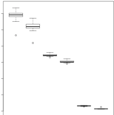
3.3 Time step sensitivity analysis, using a single zone non-residential building, highlighting the effects of different time steps when using No-MASS, 100 replicates each . . . 23

3.4 EnergyPlus, FMU Data Flow Diagram . . . 24

3.5 No-MASS Data Flow Diagram . . . 26

3.6 FMI Interface Flow Diagram . . . 27

3.7 Main DesignBuilder interface . . . 28

4.1 Residential ground floor (left), Residential 1st floor (middle), Office (Right) 38 4.2 Convergence of mean heating demand: Geneva Office (left) and House (right), 95% confidence interval . . . 41

4.3 Simulation results for yearly heating demand (Boxplot) Stochastic agent platform 100 replicates, (Circle) Single deterministic simulation . . . 43

4.4 Simulation results for monthly heating demand, (Left) Geneva Office, (Right) Nottingham Office. (Boxplot) Stochastic agent platform 100 replicates, (Circle) Single deterministic simulation. . . 44

4.5 Monthly average window state, stochastic 100 replicates, Geneva Office (Left), Nottingham Office (Right). . . 44

4.6 Monthly average light state, stochastic 100 replicates, Geneva Office (Left), Nottingham Office (Right) . . . 45

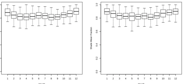
4.7 Monthly Average external shade opening fractions, stochastic 100 replicates, Geneva Office (Left), Nottingham Office (Right) . . . 45

4.8 Monthly window and heating usage for the rooms of the Geneva House. . . 46

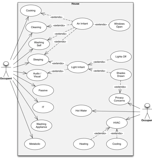
5.1 Use case diagram of occupant interactions in residential building . . . 61

5.2 Use case diagram of occupant interactions in non-residential building . . . . 62

5.3 No-MASS belief set diagram. . . 66

5.4 The light influenced privacy plan, used within the household to achieve goal 5.2.9 . . . 71

5.5 Sleeping privacy plan. . . 72

5.6 Sleeping lighting plan . . . 72

5.7 Sleeping window plan, the not sleeping state is used to depict any of the other eight states . . . 73

5.8 State diagram washing oneself with privacy consideration . . . 73

(9)

List of Figures viii

5.9 Washing self plan to open window once washing has completed, the not

washing self state is used to depict any of the other eight states . . . 74

5.10 Window open during cooking plan to remove any odours from the air . . . 74

5.11 Plan for deploying shading during the audio/visual state to reduce glare on the televisions . . . 75

5.12 Plan for appliance usage during non-residential building use . . . 76

5.13 BDI Rules’ Sensitivity Analysis, 100 replicates with the plans executing 100% of the time . . . 77

5.14 Box plots of demands due to electrical appliance rules . . . 80

5.15 Stochastic occupancy profile (dashed line) with electrical demand from com-puter(s) (solid line) . . . 80

6.1 Heating demand in a non-residential for each individual window opening model with coefficients estimated for a range of individual occupants (Haldi, 2010) and assigned to an agent profile . . . 91

6.3 Heating demand in a residential for each individual window opening model with coefficients estimated for a range of individual occupants (Haldi, 2010) and assigned to an agent profile . . . 94

7.1 Heating demand mean convergence for the learning heating setpoint within the non-residential building . . . 104

7.2 Learnt monthly heating setpoint profiles from 100 replicates within the non-residential building . . . 105

7.3 Box plots of 100 replicates for learning heating setpoints within the non-residential building . . . 106

7.4 Density plot of PMV for learning heating setpoints within the non-residential building . . . 107

7.5 Box plot of monthly mean air temperature (◦C) for the learning heating setpoints for the residential building . . . 108

7.6 Box plots of 100 replicates for learning heating setpoints within the residen-tial building . . . 109

7.7 Density plot of PMV for learning heating setpoints within the residential building . . . 109

7.8 Heating demand for mean convergence for learning window interactions . . 110

7.9 Box plots of 100 replicates for learning window interactions within the non-residential building . . . 111

7.10 Density plot of PMV for learning window interactions within the non-residential building . . . 111

7.11 Box plots of the percentage of time the window is open per month for 100 replicates in the non-residential building . . . 112

7.12 Box plots of 100 replicates for learning window interactions within the res-idential building . . . 113

7.13 Density plot of PMV for learning window interactions within the residential building . . . 113

7.14 Box plots of the percentage of time the window is open per month for 100 replicates in the residential building . . . 114

A.1 Design a Building. . . 121

A.2 Enabled detailed occupancy . . . 122

(10)

List of Figures ix

A.4 Edit the occupancy profile . . . 123

A.5 Edit individual occupants profiles, selecting windows, shades, etc.. . . 124

A.6 Run a simulation and view the results of stochastic occupancy . . . 124

C.1 Learnt monthly heating setpoint profiles from 100 replicates, Kitchen . . . . 130

C.2 Learnt monthly heating setpoint profiles from 100 replicates, Living Room . 131

C.3 Learnt monthly heating setpoint profiles from 100 replicates, Bathroom . . 132

C.4 Learnt monthly heating setpoint profiles from 100 replicates, Master Bedroom133

C.5 Learnt monthly heating setpoint profiles from 100 replicates, Residential Office . . . 134

(11)

(12)

List of Tables

4.1 Agent states with corresponding locations and values . . . 33

4.2 Residential Building Zone Details . . . 39

4.3 Non-Residential Building Zone Details . . . 39

4.4 Construction Materials . . . 40

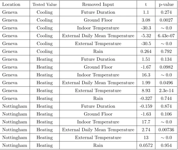
4.5 Models included in simulation compared to the base case simulation (de-grees of freedom = 99 and where p-value is∼0.0 it is less than 2.2e-16) . . 48

4.6 Window Input Parameter Sensitivity Analysis on non-residential building (degrees of freedom = 99 and where p-value is∼0.0 it is less than 2.2e-16) 50 4.7 Window Input Parameter Sensitivity Analysis on residential building (de-grees of freedom = 99 and where p-value is∼0.0 it is less than 2.2e-16) . . 51

4.8 Shade Input Parameter Sensitivity Analysis (degrees of freedom = 99 and where p-value is ∼0.0 it is less than 2.2e-16) . . . 52

4.9 Lights Input Parameter Sensitivity Analysis (degrees of freedom = 99 and where p-value is ∼0.0 it is less than 2.2e-16) . . . 52

5.1 Use Case Diagram Symbology . . . 60

5.2 Agent Services . . . 64

5.3 Agent predicates and corresponding functions . . . 67

5.4 State Chart Symbology . . . 70

5.5 BDI Rules’ Sensitivity Analysis . . . 79

6.1 Agent Voting Power . . . 88

7.1 Example Q-table table space, (*) indicates current state at 11◦C where the largest value is an action of 21◦C. . . 100

(13)

(14)

Chapter 1

Introduction

The resources needed to sustain the world’s ever expanding population are reaching new levels. In 2015, representatives from 195 countries signed an agreement with the aims of:

“Holding the increase in the global average temperature to well below 2 ◦C above pre-industrial levels and pursuing efforts to limit the temperature in-crease to 1.5◦C above pre-industrial levels, recognizing that this would signif-icantly reduce the risks and impacts of climate change;

Increasing the ability to adapt to the adverse impacts of climate change and foster climate resilience and low greenhouse gas emissions development, in a manner that does not threaten food production; and

Making finance flows consistent with a pathway towards low greenhouse gas emissions and climate-resilient development.”

(United Nations,2015) It is therefore important to reduce global energy use arising from the contribution of fossil fuels and the associated emission of greenhouse gasses.

In Europe the energy used within residential sector and the services sector accounted for 41% of the total energy used in 2013 and represented an increase of 5% relative to 1990 levels (Figure 1.1). Building performance simulation is used to model the flows of energy in buildings and their systems at the design/ retrofit stage, to ensure they not only meet the demands of the occupants but also allow designers to test strategies for improving building performance.

(15)

Chapter 1. Intr o duction 2

(16)

Chapter 1. Introduction 3

Although a powerful building (re-)design decision support tool, building performance sim-ulations can be subject to limitations. Studies have found that buildings may use twice as much energy as predicted at design stage. Bordass et al. (2001) studied 16 buildings which were predicted to have low energy use, however real world tests showed they were not low energy, but used as much as an average building. Under the stringent design and construction standards imposed by Passivhaus,Blight and Coley(2013) observed that on average a difference of 21% between simulated and actual energy use. It has been reported that for high energy buildings such as labs there is on average a factor of 2.5 difference between predicted and actual energy use (Turner and Frankel,2008). Baker and Steemers

(2003) found that building design parameters such as the plan, orientation and facade have been found to cause fluctuations in energy from 2.5 times. System parameters such boiler efficiency bring fluctuations to 5 times, leaving occupants to account for the other half of the 10 times fluctuation in energy.

Predicted building performance continues to deviate – sometimes considerably – from that which is observed post-build. The reasons are many and complex. These can be cat-egorised as (Chapman et al.,2016): (type I) errors in modelling deterministic phenomena or indeed the neglect of these phenomena, (type II) errors in the inputs to these deter-ministic models, (type III) errors in modelling stochastic phenomena or indeed the neglect of these phenomena, (type IV) errors in the inputs to these stochastic models. Type I errors might include ignoring thermal storage in the modelling of heat diffusion, assuming thermophysical properties to be constant in the dynamic modelling of heat diffusion, or assuming that heat diffuses exclusively in one direction. Type II errors might relate to the characterisation of the bulk thermophysical properties of building materials, or assuming that multilayer constructions are perfectly homogenous and known; where as in reality workmanship is imperfect and unknown. Type III errors can be sub-categorised accord-ing to whether stochastic perturbations to heat flows in buildaccord-ings are a) climatic, or b) human-behavioural in nature. Type IIIa errors might relate to wind pressures across the envelope and the corresponding impacts on convective heat transfers and infiltration, or the effects of cloud cover on transmitted shortwave irradiation. Whereas, type IIIb might relate to occupants’ presence and associated metabolic heat gains, interactions with the envelope (e.g. windows and blinds), lights, appliances and systems. Finally, type IV errors relate to the empirical coefficients that are estimated for the models that are structured to address type III errors and their suitability to the particular context under considera-tion. Thus, and as with deterministic phenomena, with respect to stochastic phenomena a distinction is made between the model structure and its ability to capture the underly-ing stochastic phenomena in principle, and the calibration of this model to a particular circumstance.

(17)

Using suitable calibration techniques simulations can more accurately represent the ag-gregate behaviour of a real building, improving predictions to within 6% (Norford et al.,

1994). Using 5 different bespoke models of occupancy,Menezes et al. (2012) managed to improve their predictive accuracy from a 70% under prediction to a 3% under prediction. The initial model used basic deterministic schedules with the final model using monitored data for lighting, appliances and catering equipment. There is clearly a performance gap that has not been covered by deterministic techniques, this gap can be reduced with ac-curate representation of real world occupant interactions. But whilst calibration from a real world building can capture the occupant interactions taking place, it is costly and not possible at the design stage.

This thesis focuses on the simulation of people within buildings and the effects of their energy related behaviours on building performance. Building performance simulation soft-ware such as EnergyPlus (Crawley et al., 2000) and ESP-r (Clarke, 2001) tend to have deterministic rules governing occupant behaviour. The deterministic rules and schedules that typically represent occupant interactions within building performance simulation soft-ware do not necessarily emulate the mean and certainly not the variance observed in real world behaviours and the performance impacts of them. There have been attempts at addressing this (Bourgeois et al.,2006) but not in a generic and portable way.

With the objective of addressing these limitations, and following the suggestions of Robin-son et al. (2011), our approach is to use multi-agent stochastic simulation for modelling occupant behaviour; to combine stochastic models into a single package that can be used to support building and urban performance simulation using a range of software. The term agent has many meanings and has evolved over time. Agents are often described as objects within programs that control their actions based on their perceptions of the environment (Huhns and Singh,1998). Multi-agent simulation is a tool that has been developed primar-ily in the social sciences to effectively model human interaction (Bonabeau,2002, Zhang et al., 2011). Its use in the social sciences has typically been to study behaviours that emerge from bottom up interactions, allowing the creator to make judgements as to what has caused these emergent behaviours and whether they correspond with expectation from social theory. An agent should have the following properties; they should be autonomous, have social ability, perceive and react to the environment and be proactive with their choices (Wooldridge and Jennings, 1995). Each agent has rules and behaviours, making them excellent in principle at modelling group and individual interactions (Axtell,2000). This work uses multiple agents to model occupants within buildings, using a combination of statistical techniques, interaction rules and machine learning.

(18)

1.1 Hypothesis

An effective modelling strategy for simulating occupants in building perfor-mance simulation is multi-agent simulation. Simulating an occupants’ energy related behaviours through agents that make use of stochastic models, theory driven rules, social interactions and machine learning techniques.

To develop and test this hypothesis the following aims are defined:

1. Represent the stochastic nature of occupants energy related behaviours, couple stochastic models of occupant interactions with building performance simulation. 2. Ensure diversity between occupants is accounted for.

3. Develop theory driven rules using belief-desire-intention techniques for the phenom-ena for which data are absent or insufficient.

4. Enable agents to communicate through a social interaction framework.

5. Integrate machine learning techniques to enable agents to learn how to react to the environment to improve their comfort.

This latter is particularly interesting for it may open up the possibility of representing stochastic behaviours of occupants in building simulation without the need complex data hungry models.

1.2 Methodological Approach

A multi-agent simulation framework has been developed, which has been named Notting-ham Multi-Agent Stochastic Simulation (No-MASS). The No-MASS framework integrates existing stochastic models of occupant interaction into a tool that can be coupled with building or urban energy performance simulation tools. The coupling allows for simu-lated occupants to make changes within the simusimu-lated building environment and receive responses arising from the effects of the interactions which may stimulate future interac-tions. Sensitivity analysis is used to scrutinise the inputs of each stochastic model ensuring that the models have a significant impact on predicting the building performance results. Parameters that do not can be removed and the models simplified. Current stochastic models do not cover all of the energy related behaviours of occupants, therefore a belief-desire-intention (BDI) rule system is used to model other interactions, supplementing the data-driven stochastic models. For example switching off the light during sleep. Agents can have unique desires causing changes within the environment that may be in conflict

(19)

with the desires of other agents. To solve this problem an agent social interaction model is developed to govern the interactions between agents. For more complex interactions where BDI rules would be difficult to design, agent machine learning techniques are used, allowing the agent to learn how to respond to different stimuli.

1.3 Research Structure

The research context, the hypothesis and structure of the work have been set out in Chap-ter1. Chapter2begins with a review of occupant representations in building performance simulation and highlights the effects occupant interactions can have on the energy per-formance of the building. Also explored in Chapter 2, is how occupants are modelled in the domains of social sciences, economics and computer science, to observe how methods from these domains can be applied to building performance simulation. Chapter 3 dis-cusses the proof of principle framework that was developed in response to needs derived from the literature and describes how the framework interfaces with building performance simulation. Stochastic models of interaction within the framework are then tested against a case study using a deterministic representation of occupants for comparison in Chapter

4. As the availability of stochastic models of interactions do not cover every aspect of an occupant’s interaction with a building, a new approach is integrated into No-MASS for creating rule based interaction ideas based on an agent belief-desire-intention method is described and tested in Chapter 5. But often building occupants do not make changes to the environment without considering the effects on other people, so presented and tested in Chapter 6 is No-MASS’s approach for handing negotiated social interactions. In Chapter

7 machine learning techniques within agents are demonstrated allowing agents to learn how to respond to the processes taking place within a building; thus agents can choose a strategy without the need for context specific rules. Finally, in 8 this thesis closes by identifying the principle contributions to knowledge arising from this work and a discus-sion for the scope of augmenting these contributions in the future. The thesis structure is summarised in Figure1.2 below.

(20)

Chapter 1. Introduction 7 Chapter 2 Chapter 5 Chapter 6 Chapter 7 Chapter 3 Chapter 4 Chapter 1 Building Performance Simulation Multi Agent Simulation No-MASS

Belief Desire Intent

Social Interactions Machine Learning Stochastic Models Introduction Chapter 8 Conclusion AIM 1 & 2 AIM 3 AIM 5 AIM 4 THE FRAMEWORK BACKGROUND

(21)

(22)

Chapter 2

Occupants in Building

Performance Simulation

This thesis focuses on the development and application of a new simulation platform, conceived to systematically improve upon the representation of type IIIb and associated type IV errors in building simulation the were identified in Chapter 1. In this endeav-our, work begins with a quick review of building simulation tools. Then the Empirical evidence maintaining that human behaviour impacts building’s performance is presented. In conjunction with this evidence the corresponding progress made in the development of stochastic models of human behaviour to address these impacts is presented. Finally, the use of agents to model people in other fields is discussed.

2.1 Building Performance Simulation

There are many building performance simulation tools often with competing algorithms and methodologies, but they all aim to support the building designer in the testing of strategies to improve the buildings performance; to reduce energy use whilst maintaining comfort and ensuring that the design is robust.

In the United States there were initially two government funded building performance simulation tools that had very similar capabilities (Crawley et al., 2001). DOE-2 and BLAST both simulated the performance of buildings but had different features that made one better in some cases and the other better in others, for example BLAST was better at systems simulation and DOE-2 better at building simulation. They were developed over many years, making them costly to maintain and so the respective developer teams pooled their resources, taking the best parts of both tools and developed a single application

(23)

Chapter 2. Occupants in Building Performance Simulation 10

named EnergyPlus. EnergyPlus can simulate surface/ air heat transfers and included a building systems manager to manage heating ventilations and air conditioning (HVAC), electrical equipment, air loops and photovoltaics (PV). Now a more comprehensive open source building systems simulation platform, it has been extensively tested, and is well documented. Made accessible through a range of both free and commercial graphical user interfaces (GUIs), most notably the DesginBuilder GUI, EnergyPlus is the most widely used of all available building performance simulation tools.

The ESP-r tool is another building performance simulation tool that simulates heat, mois-ture and air flow, electrical power flow, HVAC systems and lighting and renewable energy systems. It can also calculate performance appraisal measures such as life cycle analy-sis, indoor air quality, thermal comfort and environmental impact (Clarke, 2001). It has also been extended to simulate occupant interactions using sub hourly occupancy controls (Bourgeois et al., 2006) and computation fluid dynamics has been integrated. Although powerful, it is also complicated and unproductive to use by non-experts and, although open source, is relatively poorly documented, limiting its uptake.

TRNSYS is a modular transient simulation program initially developed for the study of solar energy systems. The main library consists of 150 models that support weather data processing, building performance simulation, the simulation of solar thermal processes and HVAC systems more generally. The library system makes it expandable, however unlike ESP-r and EnergyPlus it is neither free to use nor open source.

There a many other building simulation tools and because they often perform well in some areas and poorly in others comparisons between their ability to simulate the per-formance of buildings are difficult. Crawley et al. (2008) highlight that the terminology used throughout the different simulation tools make it difficult to compare their abilities, however they make a good attempt at doing so. These tools although useful, our work focuses on reducing the extent of the deviations between the simulated results and the real world performance of the building.

2.2 Building Performance Deviations

Seligman et al.(1978) concluded from a study of 28 identical houses there were deviations of 2 to 1 in energy demands which is thought to be primarily caused by behavioural diversity between occupants; as the houses were themselves identical. In a study of four identically constructed houses, Bahaj et al. (2007) found that in certain periods of the year energy demands varied by a factor of six due to occupancy. In their study of 22 identical residential houses in Germany, Maier et al. (2009) have identified a factor of 2

(24)

variation in heating demand. Meanwhile, post occupancy evaluations of UK EcoHomes have found that occupants’ planned behaviour accounts for a variation of 51% in heating demand between dwellings (Gill et al.,2010). The variations due to occupancy in identical buildings highlight the difficulty in performing accurate simulations of energy performance. Design stage estimations can make predictions underperform by more than half. However, calibrating models so the simulations accurately represent the real building can improved predictions to within 6% (Norford et al., 1994). Altering the heating controls using an occupant comfort measure (predicted mean vote), Andersen et al. (2007) found that a simulated building could vary in energy use by 324% from a low consumption scenario to a high consumption scenario. Using 5 different bespoke models of occupancy,Menezes et al. (2012) managed to go from a 70% under prediction of actual energy to a 3% under prediction. The initial model used basic deterministic schedules with the final model using monitored occupant data for lighting, number and use of appliances and catering equipment.

The endeavour to reduce the performance gap by accounting for variability between oc-cupants has led to models addressing the stochastic nature of ococ-cupants’ behaviours, in-tegrated within building performance simulation software. These range from hard coded integration in the case of lighting behaviour models in Reinhart’s (2004) Lightswitch2002 algorithm to Haldi and Robinson’s (2011) integration of occupant presence, window and blind models into CitySim. More recently, Vorger (2014) hard coded models of presence, activities, approximate use of heating systems, window and blind interaction within the building simulation software Pleiades+COMFIE. In line with empirical findings,Haldi and Robinson(2011) found with CitySim that variations in stochastic behaviour accounted for a factor of two variation in heating demand. Likewise, when comparing an ideal and worst case occupant scenario to demonstrate the range of influence occupants have,Roetzel et al.

(2011) found that there was a factor of 2 difference in the simulated annual energy use for both heating and cooling. Bonte et al. (2014) found a similar factor of two variation arising from the integration of models of blinds, lights, windows, temperature setpoints and clothing into a building simulation tool.

Although these efforts have usefully demonstrated the potential impact of stochastic be-haviours (and models of them) on building performance, and that these closely concur with empirical observations, they are software specific and lack generality. This criticism was partially addressed byBourgeois et al.(2006) who developed a general solution for the integration of lighting, windows and blind models with ESP-r, called Sub-Hourly Occu-pant Control (SHOCC). But this approach is also software specific and does not support more complex features.

(25)

In thesis postulates that a comprehensive behavioural modelling framework should sup-port:

“The definition of archetypes and archetypal behaviours to account for diver-sity between occupants, social interactions between members of a population and corresponding implications for their behaviours, and behaviours that are conditional on others having already been exercised or indeed on proximity to the building envelope or system, with corresponding implications for interac-tion probability.”

(Chapman et al.,2016)

2.3 Stochastic Interactions of Occupants

As noted above the endeavour to reduce the performance gap by accounting for variability between occupants has led to the development of models addressing the stochastic nature of occupants’ behaviours. Presence within a zone is a requirement for most occupant interactions within a building. Reinhart (2004) developed a simple stochastic occupancy model in the Lightswitch2002 algorithm, randomising arrival and departure times by 15 minutes from deterministic schedules. This moved the schedules away from repeated daily profiles but this is not based on empirical data. Page et al. (2008) used longitudinal occupant data to build an inhomogeneous Markov chain model to predict the likelihood of an occupant being present within a zone at a given time of day; although it does not predict movement between zones and long term absences are poorly represented (eg due to illness, business trips or vactions). More recently,Wang et al.(2011) built a Markov chain model for predicting time-dependent transitions between rooms. Chang and Hong (2013) developed curves of occupant presence based on automated lighting sensors. Finally,Feng et al.(2015) used these 3 different approaches in an algorithm where occupancy schedules are derived from Chang and Hong, the number of occupants in a room calculated using

Page et al.’s model and transitions between rooms using Wang et al.’s model. As Page et al.’s model is the only model to be rigorously validated it remains to be seen how accurate the other models are. Vorger(2014) developed probability distributions from French survey data for predicting long term absences due to holidays and sickness. Although the data is heavily influenced by the French school holidays, the same methodology could be applied to other locations.

Once occupancy is known presence dependent behaviors can be predicted. The Lightswitch2002 algorithm developed by Reinhart (2004) predicts the probabilistic use of lighting at ar-rival, during presence and at departure, as a function of minimum indoor illuminance. The

(26)

algorithm also predicts blind usage, but this is based on a deterministic solar threshold irradiance of 50W/m2. Haldi and Robinson developed two occupant interaction models, one for windows (Haldi and Robinson,2009) and one for external shading devices (Haldi and Robinson, 2010). The shading model uses a hybrid of Markov chains to predict if they are lowered or raised and a Weibull distribution to predict the opening fraction at arrival or departure. The window opening model, also uses a hybrid approach. Transitions in opening status are modelled as a discrete time Markov process, whereas the duration that a window will remain open is modelled as a continuous time random process using a Weibull distribution. Both models performed well under validation.

It is also possible to predict the activities that an occupant maybe performing at a given time. Wid´en et al. (2009) used time use survey data describing occupants’ activities to occupants activity dependent use of electrical appliances and their corresponding energy demand. Wid´en et al. (2012) expanded on this by building a Markov model to predict activities from the time use data; the outputs of which he uses in a separate model that predicts electrical demand from the activity performed. However, this model only predicts if an activity takes place not when it will start and appliances’ dynamic usage behaviour are accounted for. Wilke (2013) created a time dependent Markov chain model that predicts the transition from one activity to another at a given time, coupled with a model to pre-dict the duration for which this activity survives, from which the load profile is prepre-dicted based on that activity. Appliances are assigned based on household socio-demographic characteristics using a logistical regression based on an appliance use survey. This model performs well under validation, but it is complex and computationally expensive. In the quest for a parsimonious model (one which yields acceptable accuracy for the least compu-tational cost and complexity),Jaboob(2015) tested a range of modelling strategies, again using time use survey data, selecting time dependent Markov model of activities.

These models cover a rather comprehensive range of energy related behaviours but there remain gaps to be filled. Energy related behaviours relating to curtains interactions, window opening with regard to air quality and noise pollution, etc. To capitalise on the value of these models and to facilitate the straight forward integration of future models they should be integrated with a robust multi-agent simulation framework which is itself integrated with building performance simulation software using an open co-simulation framework. Achieving this in a coherent and generalised way is important if these models are to gain widespread use in building performance simulation, which continues to use outdated deterministic rules and schedules to support building design.

(27)

2.4 Multi-Agent Simulation

Multi-agent simulation has been used to represent people in a variety of areas. Epstein and Axtell’s (1996) SugarScape simulates a simple society where inhabitants need to eat resources in an artificial world to survive. Each agent moves around a plane looking for and consuming sugar based on predetermined rules. These models demonstrated how societies can develop over time, congregating around areas of resource. The model was expanded to include sugar and spice as resources that could be traded, from which the authors showed that the prices of both converged to an equilibrium, as economic theory would predict. Meanwhile Axelrod (1987) tested agents, employed in combination with a genetic algorithm, against a prisoner’s dilemma scenario (should you defect against or cooperate with your accomplice who has the same options). Later,Axelrod and Hamilton

(1984) found that 95% of all populations evolved towards the optimal tit-for-tat strategy, demonstrating the effectiveness of agents in exploring alternative decisions. Traffic flow within cities has also been modelled with agents, allowing traffic planners to make informed decisions to improve congestion (Balmer et al., 2006, Nagel et al.,1999). Each agent in these scenarios occupies a vehicle, with their own goals and decisions to make. Another example is city wide disaster scenarios, evaluating traffic flow during an evacuation and the effects of different city road layouts (Ring, Grid, etc.) on evacuation time (Chen and Zhan,2006). Finally,Siebers and Aickelin(2011) models the effects of changes in employee empowerment on customer satisfaction in shops.

Agent cognition is often based on the belief-desire-intention (BDI) system formulated by

Rao and Georgeff (1995). In this system an agent has beliefs about the current state of the environment and related desires about what it wants to achieve, they commit to an intent which is the desire they want to achieve. A plan, made up of a set of actions, is chosen to realise there intent. This methodology has been used in the context of building performance simulation, where agents obtain a belief about the state of the current envi-ronment from a building performance simulation tool. In this vein,Andrews et al. (2011) combine the Radiance ray tracing tool with agents, to simulate interactions with lighting and shading. Agents build up their understanding of the environment with data from Radiance (room illuminance level) then, based on their assigned personal characteristics, develop plans of actions and act on the plan that maximizes their utility (satisfaction). To simulate diversity each agent was given an archetype of either green activist, good citizen, healthy consumer or traditional consumer. These archetypes were developed from ques-tionnaires administered to building occupants, to better understand their preferred lighting levels and the energy use they are comfortable with. The agents’ assigned archetype would effect their desire thus altering their intended method of interaction. Kashif (2014) uses

(28)

a similar approach to predict the use of fridge-freezers, where an occupant would first perceive their hunger, second conceive a desire based on social normals, household rules and culture. They then finally perform an action, remove food from the freezer, increasing the electrical load on the fridge and then cook. These approaches attempt to encapsulate the human decision making processes involved in each activity. But they can lead to very complex and unwieldy models that have a weak empirical basis. Paradoxically this is also their strength, that with relatively little data reasonably reliable aggregate behaviours can be simulated.

Come what may it is important that empirical studies results have a high degree of cer-tainty and that agents’ rules and behaviours are grounded with data based on reality (Gimblett, 2002). In recent years there has been a move from models based on social theoretical rules and behaviours, to those derived from observation (Janssen and Ostrom,

2006). By using previously developed stochastic models of occupant behaviour it is pos-sible to predict agent behaviours based on solid empirical evidence. As an alternative to the BDI approach, Liao et al. (2012) use room occupancy data to inform their agents’ behaviours for the prediction of presence across multiple rooms and occupants. However,

Liao et al. note that for larger numbers of agents, it is often difficult to obtain high quality data from which to infer reliable rules. The model was also developed for a very specific use case of university buildings where students and professors have very different schedules. It has yet to be seen if this method can be applied to other building uses. Furthermore, these agents do not have the properties (social ability, reactivity and pro-activness) re-quired byWooldridge and Jennings(1995) to be formally designated as intelligent agents. More recently,Langevin et al.(2014) use data taken from a one year study of an air con-ditioned office to develop rules that allow an agent to proactively restore thermal comfort based on thermal sensation. These rules allow an agent to make changes to clothing, to operate windows/fans/heaters and to change set point temperatures. These values are then parsed to a dynamic building simulation program using the Building Control Virtual Test Bed (BCVTB). The Langevin agents are only as good as the realism given to the agent attributes specified for the model (such as clothing levels), the corresponding com-fort model and the limited thermal inhomogeneity in the simulated indoor environment. With thermal discomfort as the trigger for a specified behaviour (based on the stationary ISO 7730 model), an error in the (dis)comfort prediction will inevitably undermine the faithfulness of the predicted interactions and their consequences. An improvement would be to more explicitly represent the dynamic relationship between environmental stimuli and interactions for prediction.

In contrast with previous strategies to model occupants’ behaviour that have tended to be based either on data-driven stochastic models or BDI rules, integrated with a specific

(29)

dynamic building simulation program, this work proposes a more general framework. The virtues of both modelling approaches can be combined (data-driven where data is abundant and BDI where it is not) and interfaced with a range of building simulation programs; whether at the building or the urban scale. To this end and in the first instance, existing models of occupants’ activities, metabolic heat gains, use of windows, lights and shading devices are integrated with a bespoke platform called Nottingham Multi-Agent Stochastic Simulation (No-MASS). These agents’ interactions are parsed to a building simulation program, which in turn parses environmental parameters to No-MASS, to impact on future behaviours. This provides a generic way to integrate existing and future stochastic models, speeding up time from model development to integration and thus availability of missing models for use by the broader simulation community, increasing their usefulness. The remainder of this thesis is dedicated to describing this new framework and evolutions of it, from population generation, through parameter assignment to simulation (pre and runtime), and to demonstrating its utility.

(30)

Chapter 3

No-MASS

There remain many gaps in our ability to model occupants’ stochastic behaviours (such as their interactions with heating and cooling systems, hot water devices, curtains, their use of windows to evacuate pollutants, etc). However there is the availability of a sufficient core set of rigorously formulated and validated models with which to evaluate the proof of principle of No-MASS as a platform for addressing type IIIb and IV errors and thus of evaluating the robustness of buildings’ performance. This chapter introduces No-MASS, then discuses how it is used in the following chapters, the models included and how it is implemented. Also described is how it can be connected to other simulation tools through a generic interface, such as EnergyPlus, and finally explain its inclusion in a leading commercial building simulation tool, called DesignBuilder.

3.1 Concept

The No-MASS simulation tool was developed in two phases. The first phase (alpha) is deployed in Chapter4to test the effects of stochastic models on buildings, while the second phase (beta) is used in Chapters5 to7.

Alpha Version

The initial family of models integrated with No-MASS includes models of occupants’ ac-tivities (Jaboob, 2015), presence and corresponding metabolic heat gains (Page et al.,

2008), window interactions (Haldi and Robinson, 2009), shading interactions (Haldi and Robinson, 2010) and lighting interactions (Reinhart, 2004). These models were chosen

(31)

Chapter 3. No-MASS 18

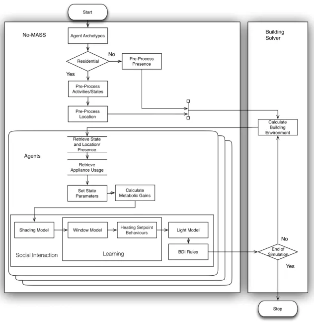
as they have been empirically verified and were readily available. Simulations with No-MASS follow the process outlined in the conceptual flow-diagram in Figure 3.1. A num-ber of pre-processes are first performed. Initially an agent population is created, with each agent assigned a profile that influences their subsequent behaviours. For example, socio-demographic characteristics influence the applicable probabilities with which time dependent activities will be predicted; likewise, the probability of being present at a given time step and the corresponding location. This maybe the agents’ office when occupying (and sleeping in) a non-residential building or their bedroom for sleeping when occupying a residential building. These characteristics and the subsequent modelling of activities is constrained in the present prototype version of No-MASS to cases of adults that act independently but whose activity choices may be influenced by the composition of the household. For example, couples may have different activity profiles than single adults liv-ing alone and elderly agents may perform different actions at different times compared with younger adults: there is a greater chance that an elderly retired occupant will be present and cook during the day, whereas a younger occupant will more likely be out at work. The profiles are defined through a simulation input file, that contains the characteristics of each agent.

Once the agents are defined a pre-process of those models that do not utilise transient environmental inputs, such as models that depend on time only, is run. A distinction between residential and non-residential buildings is made. For residential buildings the activity that an agent will perform and the corresponding location at each time step is processed; whereas in non-residential buildings, a separate presence model is used to calculate whether an agent is present in a given zone at each time step. Once these pre-processes are complete EnergyPlus is called to simulate the building’s energy flows for the first time step. At the end of each subsequent time step, No-MASS is called by EnergyPlus. Environmental conditions are parsed from EnergyPlus to No-MASS, which then uses these to predict our agents’ behaviours. Each agent is called independently and at random. For residential buildings the pre-processed activity and location for the present timestep is retrieved and used to calculate the metabolic gains for that agent and location. In non-residential buildings only the pre-processed presence is retrieved to calculate metabolic gains. Next agents’ interactions with shading devices, windows and lighting are predicted. The outputs from all models are then parsed back to EnergyPlus, which resolves the energy consequences of these interactions when simulating the building’s energy flows during the next time step, so that there is no within timestep iteration. This process continues until the end of the simulation period.

(32)

(33)

Beta Version

These core models integrated with the core version provide us with a rigorous and useful starting point, regarding the modelling of occupants’ stochastic behaviours that impact on the buildings performance. However not all such stochastic phenomena are covered. In response Figure 3.2gives an overview of an extension of the alpha version: a beta version of No-MASS with two new models included, the first a social interaction framework and the second a heating setpoint model.

As noted earlier, No-MASS builds an agent population, assigning a profile to each member dependent on the input parameters supplied in the No-MASS configuration file. These profiles are made up of the stochastic model coefficients for windows and shading, or in the case of the presence and activity model the probabilities of being in a state at a given point in time. However now an improved activity model is implemented, this allows occupant profiles to be defined through social demographical characteristics, these alter when and where the agent will be present in a household (Jaboob, 2015). These demographical characteristics consist of the agents age range, marital status, whether they are employed, their family configuration, education level and gender. A retired person will spend more time at home during the day then a professional below the age of 60, a student will sleep and wake later.

The use of shades, windows, lights and heating system setpoints are modelled via a so-cial interaction framework; which allows communication with other occupants, creating a conflict resolution mechanism and co-operative strategy. A voting system is used to allow agents to voice how they wish to interact with the environment, if the other agents in the zone agree an interaction takes place. Unlike the alpha version the social interaction model allows the stochastic models for window, shading and lighting have been moved inside the agents themselves. A benefit of this is that each agent can be given a different set of co-efficients for each model meaning more diversity between agents. Belief-Desire-Intention (BDI) rules are applied, allowing rules to be integrated where data-driven stochastic mod-els are not available. Outputs from the building solver and other modmod-els such as activities are used as inputs to deterministic rules, thus allowing No-MASS to be extended beyond the stochastic models. Finally, an agent reinforcement learning model has been introduced that can model either heating system setpoints or window interactions. Agents learn how to interact in a way that keeps discomfort to a minimum based on the temporal spacial restraints of the environment.

(34)

Set State Parameters Start

Shading Model Window Model

Pre-Process Activities/States Retrieve State and Location/ Presence Pre-Process Location Light Model No-MASS Pre-Process Presence Building Solver Stop End of Simulation Yes No Retrieve Appliance Usage Agent Archetypes Social Interaction Calculate Metabolic Gains Agents Residential Yes No BDI Rules Heating Setpoint Behaviours Learning Calculate Building Environment

(35)

3.2 Implementation

No-MASS was built from the ground up, having tested a number of current multi-agent simulation development platforms, including Repast Simphony and Anylogic. Although these platforms are very useful they come with significant overheads, typically requiring a large library of graphical user interface routines to be imported, making it more difficult to package a No-MASS equivalent with simulation tools such as EnergyPlus and the De-signBuilder interface to it. C++ was chosen as the development language as it is simple to integrate with EnergyPlus (Crawley et al.,2001), our chosen building simulation tool is also developed in C++. Using the same language allows for easy communication between the two tools. EnergyPlus developed by the US Department of Energy, is well tested, well documented and open source; allowing us to readily understand how to connect to it. There are also two interfaces that allow other tools to interact with it, without altering the EnergyPlus source code. The first is through the building controls virtual test bed (BCVTB) and the second is through the Functional Mockup Interface (FMI) (Nouidui et al., 2013). The No-MASS platform connects to EnergyPlus using FMI, which is an open standard so that No-MASS could in principle be integrated with any other FMI compliant simulation tool. This is chosen over the BCVTB as it allows direct commu-nication through C++ double precision arrays using predefined calling points, whereas BCVTB requires calls over sockets adding complexity and slowing the processing time. The calling points are well documented, with No-MASS only using theinitialise function,

the receive an array of doubles function for the environmental variables and the send an

array of doubles function for the occupant interactions. The array of values that No-MASS

receives at each time step is defined in the XML file ModelDescription.xml. At the begin-ning of the time step the following environmental variables are received: horizontal sky illuminance, rain status, outdoor air dry-bulb temperature, zone air temperature, zone humidity, indoor radiant temperature and indoor illuminance. Returned to EnergyPlus are the number of occupants in a zone, their metabolic gains, appliance gains, the window status, the blind shading fraction, the lighting status and the heating setpoint. Due to the window, shading and location/presence models used within No-MASS a sub-hourly timestep is recommended (ie. 5 minutes), as longer timesteps may overestimate the impli-cation of the occupant interactions. For example the response time to an agent opening a window may be short with the room cooling in just a few minutes. An agent can only respond at the next time step, if the timesteps are not sufficiently short in length, the open window may over cool the room. Figure3.3 shows the effects of different simulation timesteps on the performance of the simulation on a non-residential monozone building. The timestep choice will have a differing impact depending on the complexity of the build-ing and the occupants simulated.

(36)

Chapter 3. No-MASS 23 1 2 3 4 5 6 10 12 15 20 30 110 115 120 125 130 135 140 145

Length Of Timestep (Minutes)

Heating Demand (kWh/m2.y)

Figure 3.3: Time step sensitivity analysis, using a single zone non-residential building, highlighting the effects of different time steps when using No-MASS, 100 replicates each

No-MASS has been developed as both a Linux shared object and as a Microsoft Windows dynamic link library. Figure 3.4 shows how the system connects to EnergyPlus. In the same way that EnergyPlus reads in the building configuration and weather data from the IDF file and the EPW file, No-MASS reads in data from an XML file called NoMass-Config.xml. This file contains information about the occupants that is used to build the agent population, and the subsequent processing of an agent activity profile (a series of parameters defining the the socio-demographic characteristics of the agent, ie. gender, age, income level, etc) that is used to calculate the probability of an activity taking place at each timestep, as well as the bedroom or office that this agent will assigned to during the corresponding activity (eg. the bedroom while sleeping). It also defines the window

(37)

and shading model coefficients for each model, allowing for diversity between occupants and models to be represented as needed.

Figure 3.4: EnergyPlus, FMU Data Flow Diagram

3.3 Integration

3.3.1 EnergyPlus

EnergyPlus is typical in its use of deterministic rules that represent occupant interactions within buildings. The types of interactions that can be set are limited to single event driven procedures, for example ifx happens at time tdo y. Heating setpoints in Energyplus are determined by a combination of temporal (the time and date) and comfort related eg. air temperature, operative temperature, thermal comfort (Fanger’s predicted mean vote) and humidity parameters. An example of a schedule defining the heating setpoints would

(38)

Chapter 3. No-MASS 25 be: Schedule:Compact, Kitchen Heating SP Sch, T emperature, T hrough: 31Dec, F or:W eekdays, U ntil: 05 : 00, 12, U ntil: 10 : 00, 18, U ntil: 17 : 00, 12, U ntil: 23 : 00, 18, U ntil: 24 : 00, 12;

This describes the heating setpoints for the kitchen zone for weekdays throughout the year heating the zone to 18◦C between 5am to 10am and 5pm to 11pm, and to 12◦C otherwise. For window openings the interactions are set in a similar schedule format, albeit with more parameters to choose from (including air temperature, enthalpy, constant, thermal comfort (ASHRAE 55 adaptive and CEN 15251 adaptive), adjacent temperature and adjacent enthalpy). Shading interactions are enabled through a schedule then set through a single setpoint value, either a temperature for heating or cooling, or solar irradiance incident either at the window or on the horizontal plane. Lights are set though a fraction schedule where the values are a fraction of the design level to allow for dimming. Presence within a zone is also set through schedule of the fraction of the total number of occupants that can occupy a zone.

Functional Mockup Interface (FMI)

No-MASS couples with EnergyPlus through the open FMI standard, a generic program-ming interface that allows other programs to interface to EnergyPlus to extend its func-tionality. It provides a description of how information can be passed from EnergyPlus at runtime to a functional mockup unit (FMU) which can then make calculations, the results of which are parsed back to EnergyPlus. These results are then used by EnergyPlus for future calculations.

An FMU consists of:

• The FMU Library (Windows Dynamic Link Library, Linux Shared Object) • A Model Description File

(39)

• Any Other Configuration Files

The library file contains the programmed equations, in a programming language that supports C interfaces. When the No-MASS source code is compiled it is in the form of the library file. No-MASS works as both a Windows dynamic link library or a Linux Shared object. It can also be compiled on Macintosh computers; however EnergyPlus does not support FMI on Macintosh computers so no testing has been conducted on the MacOS.

FMI works using a simple data exchange methodology (Figure 3.5). At each timestep EnergyPlus sends a set of predefined variables (x) to the FMU (e.g. Zone Mean Air Temperature and/or Site Rain status). The FMU performs a calculation on the values and returns a set of results (y) to EnergyPlus (e.g. occupant location and/or shade status). These return values can be made to overwrite EnergyPlus values for the next timestep.

Figure 3.5: No-MASS Data Flow Diagram

Within EnergyPlus there are three types of external interface that can be written to:

ExternalInterf ace:F unctionalM ockupU nitImport:T o:V ariable

ExternalInterf ace:F unctionalM ockupU nitImport:T o:Schedule

ExternalInterf ace:F unctionalM ockupU nitImport:T o:Actuator

No-MASS uses the schedules and actuators to write values to EneryPlus, overwriting the predefined deterministic rules, at each timestep. The flow of processing from EnergyPlus to the FMU is given in Figure 3.6.

(40)

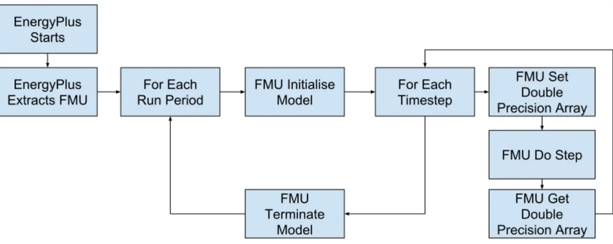
Chapter 3. No-MASS 27 EnergyPlus Starts EnergyPlus Extracts FMU For Each Timestep For Each Run Period FMU Initialise Model FMU Set Double Precision Array FMU Do Step FMU Get Double Precision Array FMU Terminate Model

Figure 3.6: FMI Interface Flow Diagram

EnergyPlus starts, reads in its configuration file, and determines that it needs to run a simulation for use with an FMU. EnergyPlus then searches for the FMU, in this case No-MASS, and extracts the information it needs to communicate with the FMU. For each run period the FMU is initialised by calling the initialise method of the FMU. Then at each timestep EnergyPlus calls the FMU, setting the variables in the FMU by passing an array of double precision values defined in the model description XML file. Then EnergyPlus calls the FMU do step method where the FMU performs any calculations (see Figure 3.1

for the processes inside No-MASS). To receive the return values EnergyPlus calls the get double precision array method in the FMU and receives an array of double precision values back, as specified in the model description XML file. Once all timesteps are completed the FMU is terminated and the simulation is ended.

(41)

DesignBuilder

Figure 3.7: Main DesignBuilder interface

.

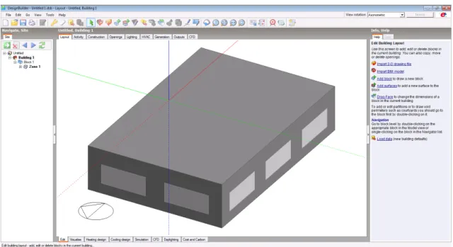
DesignBuilder provides access to EnerygPlus through an easy-to-use interface that serves more than 3500 customers in 80 different countries. Their main market sectors are ser-vices engineers, building simulation experts, architects (technical), energy assessors (UK), LEED, BREEAM, Green Star assessors, university R&D and teaching. To enable re-searchers and early adopters to use and test MASS, GUI components controlling No-MASS were integrated with the DesignBuilder GUI (See AppendixAfor screen shots of the tool in use). In this way No-MASS can now in principle be used by any building designer without the need to know the complexities of EnergyPlus, FMI, and No-MASS.

The steps in developing and simulating a No-MASS compliant model are as follows: Using the DesignBuilder GUI a building is designed. A user can then enable the No-MASS occupants in the simulation configuration dialogue. Once enabled on the main occupant activity screen there are a choice of occupant templates. There are predefined sets of occupants for offices or residential buildings (eg. family with children, working professional, students, retired, etc.) that can be chosen. Each set of occupants can be further edited allowing different combinations of presence, activities, shades and windows profiles to be defined. The current limitations of the GUI are that it does not allow for agent learning and as of yet BDI rules have not been added.

This tool allows for quick and easy setup of complex building types with differing stochastic occupants. A designer can now test the building against a range of different use cases, with

(42)

occupants simulated as agents and interactions based on real world empirical, validated models and data.

(43)

(44)

Chapter 4

Data Driven Stochastic Models,

Coupled with Building

Performance Simulation

No-MASS couples stochastic models of occupant interaction with building simulation, the process of which was described in the previous chapter. This chapter describes how these models work and the effects they have on building performance. The models are also analysed in terms of their inputs to ensure that each has a significant effect on building performance.

4.1 Stochastic Models

Activity model

The activity model (Jaboob, 2015) predicts the time-dependent probability that one of a set of ten activities will be performed in the home. These activities include sleeping, passive, audio/visual, IT, cooking, cleaning, metabolic, washing appliance use, personal washing and absence from the building. The activities were derived from the UK Time Use Survey (TUS) data 2000-2001 (Gershuny and Fisher, 2013). Jaboob’s work was to better predict activity-dependent use of energy in homes. The data was filtered into 10 activities, those within the home aggregated into a set of nine meta activities, with activities taking place outside of the home aggregated into a single activity, out of the home. This formulation of 10 energy-related activities reduced the risk of over-fitting in their model. Most of these activity aggregates are self-explanatory, however some are

(45)

Chapter 4. Data Driven Stochastic Models 32

less so. The activity passive refers to occasions when an occupant is awake, but not physically active; whereas metabolic refers to when an occupant is awake and physically active. After implementing and testing a number of different prediction methodologies

Jaboob (2015) found that modelling the activities as a time-dependent Bernoulli process using multinomial logistic regression was the most parsimonious (good predictions and least computationally expensive) approach.

P(x, t) = exp(Aj(x, t)) ΣN_j₌₁exp(Aj(x, t)), j = 1, . . . , N (4.1.1) and Aj(x) =αj+ n X k=1 βjkxjk (4.1.2)

Where, t is time, N corresponds to the total number of activities, n the number of pre-dictors, and x the predictors describing the observation, each associated with a slope coefficientβjk, andαj is the intercept. As the probabilities are only dependent on time it is possible to generate a 10 by 24 matrix giving the probability of performing each activity at a given hour; though the corresponding model can also be re-called within the hour for sub-hourly simulation timesteps. Models can also be estimated for subpopulations of the time use survey dataset from which they are derived, to give probabilities that depend for example on age, employment status, season or day of the week. No-MASS accounts for diversity through a choice of sub-models, for the activity model a range of occupants defined through social demographical characteristics can be chosen, these alter when the where the agent will be present in a household. A retired person will spend more time at home during the day then a professional below the age of 60. The sub-model used for each agent is assigned when the agent population is generated. This model is pre-processed, assigning a state to each timestep within the simulation. This is achieved by drawing a random number for each timestep for each agent. Where that number falls within the range of probabilities for that hour, the corresponding activity is assigned to the relevant agent. These are then stored for retrieval at run time.

Note that this process is only considered for residential buildings and does not apply to the simulation of non-residential buildings, for which the corresponding time use survey data is not available. Jaboob (2015) also provides predictions for secondary activities, for example audio/ visual while cooking. However these have not yet been integrated; currently No-MASS infers location, clothing level and metabolic rate from the activity model, thus there would be no energy related consequences of the second action.