Robust methods in Mendelian
randomization
Jessica Mary Barbara Rees
Department of Public Health and Primary Care
University of Cambridge
This dissertation is submitted for the degree of
Doctor of Philosophy
Declaration
This thesis is the result of my own work and includes nothing which is the outcome of work done in collaboration except as declared in the Acknowledgements and specified in the text. It is not substantially the same as any that I have submitted, or, is being concurrently submitted for a degree or diploma or other qualification at the University of Cambridge or any other University or similar institution except as declared in the Acknowledgements and specified in the text. I further state that no substantial part of my thesis has already been submitted, or, is being concurrently submitted for any such degree, diploma or other qualification at the University of Cambridge or any other University or similar institution except as declared in the Acknowledgements and specified in the text. It does not exceed the prescribed word limit for the relevant Degree Committee.
Jessica Mary Barbara Rees January 2019
Robust methods in Mendelian
randomization
Jessica Mary Barbara Rees
Mendelian randomization uses genetic variants as instrumental variables to estimate the causal effect of a risk factor on an outcome using observational data. If a genetic variant is included in a Mendelian randomization study that does not satisfy the instrumental variable assumptions then the causal estimate from traditional instrumental variable methods will be biased. Since Mendelian randomization studies using publicly available summary level data (estimates and standard errors of the genetic associations with the risk factor and the outcome) from large consortia can be performed with relative ease and little expense, the popularity of Mendelian randomization in epidemiological studies has increased dramatically. As such, various methods have been developed in Mendelian randomization that use summary level data and account for possible violations of the instrumental variable assumptions. However, additional Mendelian randomization methods that account for violations in the instrumental variable assumptions are still required.
In this dissertation, we introduce robust methods for Mendelian randomization that downweight the contribution of genetic variants with heterogeneous causal ratio estimates. We extend the univariable MR-Egger method to the multivariable setting to account for both measured and unmeasured pleiotropic effects. We also explore the possibility of extending multivariable Mendelian randomization to the factorial setting to estimate statistical interaction effects. Finally, we apply some of the methods we have developed to perform a Mendelian randomization study to investigate the effect of adiposity and body composition measurements on asthma using data from UK Biobank and the GABRIEL consortium.
This dissertation is dedicated to my uncle, Canon Peter Coyle, who passed away during my PhD. He will always be remembered for his kindness, humility, and
Acknowledgements
I would like to thank my supervisor, Stephen Burgess, for his guidance and support, and my secondary supervisor, Angela Wood, for advice and feedback on the work presented in this dissertation. I would also like to thank Chris Foley for helpful discussions and contributions to the work presented in Chapter 5, and Raquel Granell for feedback on the work in Chapter 6.
The work presented in Chapter 3 is based on work originally carried out by my supervisor Stephen Burgess and other collaborators (Jack Bowden, Frank Dudbridge and Simon Thompson). A copy of a draft manuscript that has been uploaded to arXiv on this work by Stephen Burgess and colleagues can be found in Appendix A. I acknowledge that Stephen Burgess developed the methods in Sections 3.3.1 to Section 3.3.3. I suggested the extension in Section 3.3.4, performed the additional applied analysis in Section 3.4, adapted and re-performed the simulation studies, and re-wrote the work. I would like to thank Stephen Burgess, Angela Wood, Jack Bowden and Frank Dudbridge for their useful comments on the work contained in Chapter 3. The paper in Appendix B is based on the work in Chapter 3 and was written by me under the supervision of Stephen Burgess, with contributions from Angela Wood, Jack Bowden and Frank Dudbridge.
The paper in Appendix D was written by me under the supervision of Stephen Burgess, with contributions and editorial input from Angela Wood. This paper forms the basis of the work in Chapter 4.
The paper in Appendix F was written by me under the supervision of Stephen Burgess, with contributions from Chris Foley. This paper forms the basis of the work in Chapter 5.
Finally, I would like to thank my family and friends for all their help and encour-agement. I would particularly like to acknowledge the unwavering support shown by my parents, Andrew and Margaret.
Abbreviations
AD Alzheimer’s disease
ATE average treatment effect
BIA bioelectrical impedance analysis
BMI body mass index
CHD coronary heart disease
CI confidence interval
DAG directed acyclic graph
DXA dual X-ray emission absorptiometry
FEV1 forced expiratory volume in 1 second FFM/FFMI fat free mass/fat free mass index
FM/FMI fat mass/fat mass index
FVC forced volume vital capacity
GABRIEL Multidisciplinary Study to Identify the Genetic and
Environmental Causes of Asthma in the European Community GIANT Genetic Investigation of ANthropometric Traits
GLIDE global and individual tests for direct effects
GLGC Global Lipids Genetics Consortium
GWAS genome-wide association study
GWS genome wide significance
HDL-C high-density lipoprotein cholesterol
InSIDE instrument strength independent of direct effect
ITT intention to treat
IV instrumental variable
IVW inverse-variance weighted
LDL-C low-density lipoprotein cholesterol
LM/LMI lean mass/lean mass index
LP Lasso penalization
LTS least trimmed squares
MAF minor allele frequency
MBE mode-based estimator
MR-Egger Mendelian randomization-Egger
NOME no measurement error
OLS ordinary least squares
OR odds ratio
PC principle component
PW penalized weights
QC quality control
RCT randomized clinical trial
Rr robust regression
RR relative risk
xi
SD standard deviation
SE standard error
SNP single nucleotide polymorphism
SSGAC Social Science Genetic Association Consortium
TAG Tobacco, Alcohol and Genetics
TSLS two-stage least squares
Notation
X risk factor
¯
X mean value of the risk factor (Chapter 5)
Y outcome
U confounder of theX−Y association
Z instrumental variable
G genetic variant acting as an instrumental variable
UI univariable inverse-variance weighted (Chapter 4) UE univariable MR-Egger (Chapter 4)
MI multivariable inverse-variance weighted (Chapter 4) ME multivariable MR-Egger (Chapter 4)
GS weighted gene score
α direct effect of Gon Y
α′ direct effect of Gon Y in a multivariable framework (Chapter 4) βX parameter of genetic association: regression parameter in the
G−X regression
βY parameter of genetic association: regression parameter in the G−Y regression
γ causal effect of one risk factor on another risk factor (Chapter 4) δ parameter of genetic association: regression parameter in the
G−U regression (Chapter 3)
ζX parameter of genetic association: regression parameter in the U−X regression
ζY parameter of genetic association: regression parameter in the U−Y regression
ϵ error term in linear regression models θ causal effect of X onY
θM marginal causal effect of X onY (Chapter 5) λ penalty term in Lasso regression (Chapter 3)
µ mean value of α′ (Chapter 4) or mean value of X (Chapter 5)
ρ correlation parameter
σ variance parameter
φ random effects parameter
F F statistic from regression ofX onG
h number of data points in least trimmed squares (Chapter 3) i subscript indexing individual
j subscript indexing genetic variant J total number of genetic variants
k subscript indexing risk factor (Chapter 4) K total number of risk factors (Chapter 4) N total number of individuals or observations
xiii
p probability of Y (Chapter 5)
Q Cochran’s Q statistic
r standardised residuals (Chapter 3)
r2 measure of linkage disequilibrium (Chapter 6)
R2 amount of variance explained in X
w inverse-variance of the causal ratio estimate
wLT S weights from least trimmed squares regression (Chapter 3)
B binomial distribution
N normal distribution
U uniform distribution
χ2 chi-squared distribution
Table of contents
v
List of figures xxi
List of tables xxv
1 Introduction 1
1.1 Causal effect . . . 1
1.2 Randomized clinical trials . . . 2
1.3 Epidemiological studies . . . 2
1.4 Instrumental variable analyses . . . 3
1.5 Mendelian randomization . . . 4
1.5.1 Using genetic variants as instrumental variables . . . 5
1.5.2 Classification of studies . . . 6
1.6 Motivation for the dissertation . . . 7
1.7 Structure of the dissertation . . . 9
2 Statistical methods for Mendelian randomization 11 2.1 Testing for a causal effect . . . 11
2.2 Additional assumptions for a point estimate . . . 12
2.3 Estimating the causal effect . . . 13
2.3.1 Wald (ratio) estimator . . . 14
2.3.2 Two-stage least squares regression . . . 16
2.3.3 Binary outcomes . . . 16
2.4 Pleiotropic genetic variants . . . 17
2.5 Heterogeneity and pleiotropic variants . . . 19
2.5.1 Plots of the genetic associations . . . 19
2.5.2 Test for heterogeneity . . . 21
2.6 Sensitivity analyses . . . 22
2.6.1 Downweighting or removing genetic variants . . . 22
2.6.2 MR-Egger . . . 25
2.6.3 Multivariable Mendelian randomization . . . 30
2.7 Conclusion . . . 35
3 Robust methods for Mendelian randomization 37 3.1 Introduction . . . 37
3.2 Robust statistics and Mendelian randomization . . . 38
3.2.1 Overview of robust statistics . . . 39
3.2.2 Relevance of robust statistics to Mendelian randomization . . . 39
3.2.3 Methods considered . . . 40
3.3 Methods . . . 40
3.3.1 Robust regression (MM–estimation) . . . 41
3.3.2 Penalized weights . . . 44
3.3.3 Lasso selection . . . 46
3.3.4 Least trimmed squares selection . . . 48
3.3.5 Binary outcomes . . . 49
3.3.6 Summary and overview of methods . . . 49
3.4 Applied examples . . . 51
3.4.1 Causal effect of body mass index on schizophrenia risk . . . 51
3.4.2 Causal effect of low-density lipoprotein on Alzheimer’s disease risk 52 3.4.3 Results . . . 52
3.4.4 Summary . . . 54
3.5 Simulation study . . . 59
3.5.1 Data generating model . . . 59
3.5.2 Methods applied to the simulated data . . . 61
3.5.3 Results . . . 62
3.5.4 Increased number of genetic variants . . . 71
3.5.5 Binary outcome . . . 75
3.5.6 Summary . . . 81
3.6 Discussion . . . 82
3.6.1 Comparison with the arXiv paper . . . 83
3.6.2 Interpretation of heterogeneity among the causal ratio estimates 83 3.6.3 Issues with penalizing genetic variants . . . 84
3.6.4 Implication for Mendelian randomization studies . . . 84
Table of contents xvii
3.6.6 Key points from chapter . . . 86
4 Multivariable MR-Egger 89 4.1 Introduction . . . 89
4.2 Methods . . . 90
4.2.1 Univariable Mendelian randomization . . . 91
4.2.2 Multivariable Mendelian randomization . . . 93
4.2.3 Assumptions for multivariable MR-Egger . . . 95
4.2.4 Precision of the multivariable MR-Egger estimate . . . 96
4.2.5 Advantages of multivariable MR-Egger and comparison with univariable MR-Egger . . . 97
4.2.6 Orientation of the genetic variants . . . 98
4.2.7 Summary . . . 99
4.3 Causal effect of HDL-C on CHD risk . . . 100
4.3.1 Methods . . . 100 4.3.2 Results . . . 101 4.3.3 Summary . . . 103 4.4 Simulation study . . . 104 4.4.1 Results . . . 109 4.4.2 Summary . . . 112
4.5 Causal relationships between risk factors . . . 113
4.5.1 Simulation study . . . 113
4.5.2 Summary . . . 118
4.6 Discussion . . . 119
4.6.1 Multivariable by design, or multivariable as a sensitivity analysis?119 4.6.2 InSIDE assumption and orientation of genetic variants . . . 120
4.6.3 Linearity and homogeneity assumptions . . . 121
4.6.4 Implication for future research . . . 122
4.6.5 Correlated genetic variants . . . 123
4.6.6 Key points from chapter . . . 124
5 Factorial Mendelian randomization 125 5.1 Introduction . . . 125
5.2 Interaction effects . . . 126
5.2.1 Factorial randomized clinical trials . . . 126
5.2.2 Interaction effects using observational data . . . 129
5.2.4 Summary . . . 132
5.3 Factorial framework . . . 132
5.3.1 Genetic variants used as predictors for the risk factors . . . 132
5.3.2 Genetic variants acting as proxies for pharmacological interventions133 5.3.3 Effect of obesity and alcohol consumption on the risk of liver disease . . . 135
5.3.4 Requirement for further methodological research . . . 136
5.3.5 Summary . . . 138
5.4 Performing factorial Mendelian randomization . . . 138
5.4.1 Genetic variants used as predictors of risk factors . . . 139
5.4.2 Genetic variants used as proxies for drug treatments . . . 164
5.4.3 Summary . . . 172 5.5 Applied example . . . 172 5.5.1 Methods . . . 173 5.5.2 Results . . . 175 5.5.3 Summary . . . 177 5.6 Discussion . . . 178
5.6.1 Interpretation of the interaction effect . . . 179
5.6.2 Strength of the instrumental variables . . . 179
5.6.3 Number of cross-over variants . . . 180
5.6.4 Dichotomization of the gene scores . . . 180
5.6.5 Limitations . . . 181
5.6.6 Key points from chapter . . . 182
6 Applied example: adiposity and asthma 183 6.1 Introduction . . . 183
6.1.1 Motivation . . . 184
6.1.2 Measurements for adiposity and body composition . . . 185
6.1.3 Genome wide association studies on adiposity, body composition and asthma . . . 186
6.1.4 Study design . . . 186
6.1.5 Summary . . . 189
6.2 One–sample Mendelian randomization analysis . . . 191
6.2.1 Exposure and outcome measurements . . . 192
6.2.2 Data quality control . . . 193
6.2.3 Selection of genetic variants . . . 196
Table of contents xix
6.2.5 Mendelian randomization analyses . . . 204
6.2.6 Descriptive statistics of the individual level data . . . 206
6.2.7 Summary level data . . . 210
6.2.8 Ever diagnosis of asthma . . . 213
6.2.9 Current asthma . . . 216
6.2.10 Summary . . . 219
6.3 Two–sample Mendelian randomization analysis . . . 220
6.3.1 Methods . . . 220 6.3.2 Results . . . 224 6.3.3 Summary . . . 226 6.4 Comparison of results . . . 228 6.4.1 Univariable analyses . . . 228 6.4.2 Multivariable analyses . . . 230 6.4.3 Summary . . . 232 6.5 Discussion . . . 233
6.5.1 Measurements for asthma and body composition . . . 233
6.5.2 Instrumental variables for body composition . . . 233
6.5.3 Application of multivariable methods . . . 234
6.5.4 Limitations . . . 234
6.5.5 Key points from the chapter . . . 236
7 Conclusions and future work 237 7.1 Summary of the thesis . . . 238
7.1.1 Chapter 1 . . . 238 7.1.2 Chapter 2 . . . 238 7.1.3 Chapter 3 . . . 239 7.1.4 Chapter 4 . . . 239 7.1.5 Chapter 5 . . . 240 7.1.6 Chapter 6 . . . 241 7.2 Future work . . . 242
7.2.1 Extension to correlated genetic variants . . . 242
7.2.2 Unresolved issues for multivariable MR-Egger . . . 243
7.2.3 Multivariable methods . . . 243
7.2.4 Interaction effects . . . 244
7.3 Conclusion . . . 244
Appendix A Paper from arXiv: Robust instrumental variable methods using multiple candidate instruments with application to Mendelian
randomization 263
Appendix B Paper 1: Robust methods in Mendelian randomization via
penal-ization of heterogeneous causal estimates 309
Appendix C Appendix to paper 1 335
Appendix D Paper 2: Extending the MR-Egger method for multivariable Mendelian randomization to correct for both measured and unmeasured
pleiotropy 349
Appendix E Appendix to paper 2 365
Appendix F Paper 3: Factorial Mendelian randomization: using genetic
vari-ants to assess interactions 379
Appendix G Appendix to paper 3 393
Appendix H Chapter 3 supplementary material 407
H.1 Non-convergent robust regression models . . . 407 H.2 MR-Egger models . . . 408 H.3 One-sample Mendelian randomization . . . 410
Appendix I Chapter 6 supplementary material 413
I.1 One–sample Mendelian randomization study . . . 413 I.1.1 Histograms of the adiposity and body composition measurements413 I.1.2 Information on the genetic variants considered for the Mendelian
randomization analysis . . . 417 I.1.3 Genetic associations with the body composition measurements
and asthma . . . 420 I.2 Two-sample Mendelian randomization study . . . 433 I.2.1 Genetic associations with asthma from the GABRIEL consortium433 I.2.2 Genetic associations with BMI from UK Biobank . . . 435
List of figures
1.1 Directed acyclic graph illustrating the instrumental variable assumptions. 4 1.2 Illustration of some of the types of Mendelian randomization studies. . 7 2.1 Directed acyclic graph illustrating the Mendelian randomization
assump-tions. . . 13 2.2 Directed acyclic graph illustrating a potentially pleiotropic genetic
vari-ant that invalidates the Mendelian randomization assumptions. . . 18 2.3 Example scatter plot of the genetic associations with Alzheimer's disease
against the genetic associations with low-density lipoprotein cholesterol. 20 2.4 Directed acyclic graph illustrating the multivariable Mendelian
random-ization assumptions. . . 32 2.5 Directed acyclic graph illustrating instrument strength for multivariable
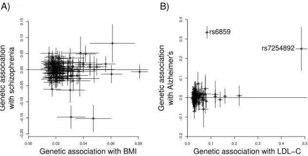
Mendelian randomization. . . 34 3.1 Scatter plots of the genetic associations with body mass index and
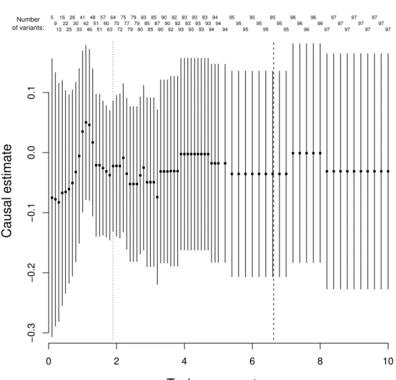
schizophrenia, and the genetic associations with low-density lipoprotein cholesterol and Alzheimer's disease. . . 53 3.2 Estimates of the approximate log causal odds ratios for schizophrenia
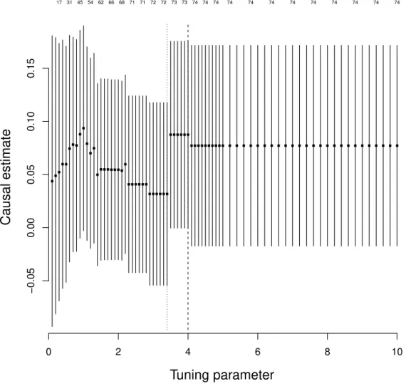
per unit increase in body mass index from the Lasso selection method. 57 3.3 Estimates of the approximate log causal odds ratios for Alzheimer's per
unit increase in low-density lipoprotein from the Lasso selection method. 58 3.4 Directed acyclic graph used in the data generating model for the
simu-lation study. . . 60 4.1 Directed acyclic graph illustrating the potential violation of the
instru-mental variable assumptions by a pleiotropic effect. . . 92 4.2 Directed acyclic graph illustrating the multivariable Mendelian
4.3 Directed acyclic graph illustrating the causal relationship between two risk factors used in the simulation study. . . 114 5.1 Figure comparing a factorial randomized clincial trial to a multivariable
Mendelian randomization study. . . 133 5.2 Directed acyclic graph illustrating a multivariable Mendelian
random-ization framework. . . 140 5.3 Histograms of the estimates and standard errors of the positive
inter-action effect from the simulation study when there were no cross-over variants. . . 148 5.4 Plot of the median standard errors of the interaction term for the four
two stage least squares regression models from the simulation study. . . 153 6.1 Directed acyclic graph illustrating the assumed relationships betweem
the risk factors and outcome for the Mendelian randomization study. . 187 6.2 Characteristics of the two Mendelian randomization studies. . . 188 6.3 Flowchart of the number of participants with phenotypic and quality
controlled genetic data from UK Biobank. . . 194 6.4 Flowchart highlighting the quality control steps applied to the genotyped
genetic data from UK Biobank. . . 195 6.5 Univariable and multivariable Mendelian randomization analyses
per-formed to investigate the effect of adiposity and body composition on asthma . . . 204 6.6 Scatter plots of the genetic associations for fat mass index and fat-free
mass index from UK Biobank. . . 212 6.7 Scatter plot of the genetic associations with body mass index and ever
diagnosis of asthma in UK Biobank for the variants used in the main analysis. . . 214 6.8 Scatter plot of the genetic associations with body mass index and ever
diagnosis of asthma in UK Biobank for the reduced set of variants used in the main analysis. . . 214 6.9 Scatter plot of the genetic associations with body mass index and current
asthma status in UK Biobank. . . 217 6.10 Scatter plot of the genetic associations with body mass index and current
asthma status in UK Biobank for the reduced set of variants. . . 217 6.11 Flowchart highlighting the number of variants with genetic association
List of figures xxiii 6.12 Scatter plot of the genetic associations with body mass index from UK
Biobank and the genetic associations with asthma from the GABRIEL consortium. . . 225 6.13 Scatter plot of the genetic associations with body mass index from UK
Biobank and the genetic associations with asthma from the GABRIEL consortium for the reduced set of genetic variants. . . 225 6.14 Forest plot comparing the estimates for body mass index from the
one–sample and two–sample Mendelian randomization studies. . . 229 6.15 Forest plot comparing the estimates for fat mass index and fat-free mass
index from the one–sample and two–sample analyses. . . 231 I.1 Histograms of weight, height and body mass index from UK Biobank. . 414 I.2 Histograms of the bioelectrical impedance analysis measurements for fat
mass index and fat-free mass index from UK Biobank. . . 415 I.3 Histograms of the dual-energy X-ray measurements for fat mass index,
List of tables
3.1 Overview of the robust methods introduced in Chapter 3. The meth-ods are categorised by whether they downweight genetic variants with heterogeneous ratio estimates (can be applied to the IVW or MR-Egger methods) or select genetic variants for the IVW method. . . 50 3.2 Estimates of the approximate log causal odds ratios for schizophrenia
per unit increase in body mass index and Alzheimer's disease per unit increase in low-density lipoprotein. . . 56 3.3 Summary statistics on instrument strength from the simulation study
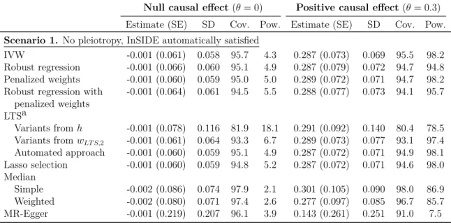
for Scenarios 1-4 with a null or positive causal effect. . . 62 3.4 Results from the simulation study for Scenario 1 with a null or positive
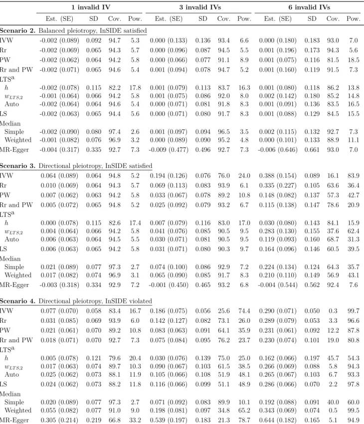
causal effect. . . 64 3.5 Results from the simulation study for Scenarios 2-4 with a null causal
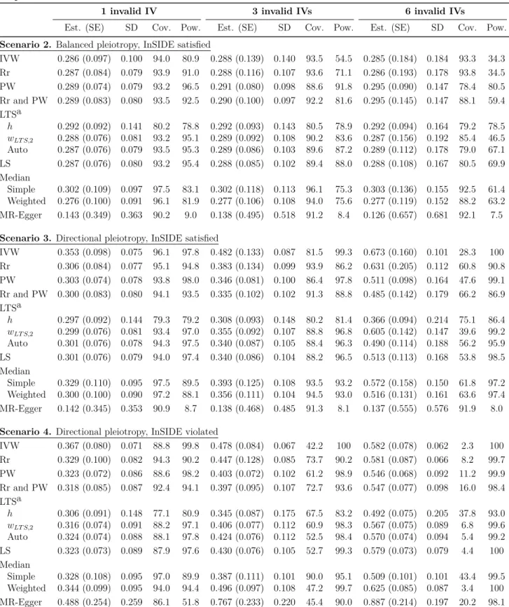
effect. . . 66 3.6 Results from the simulation study for Scenarios 2-4 with a positive
causal effect. . . 67 3.7 Power of the intercept test in the MR-Egger method from the simulation
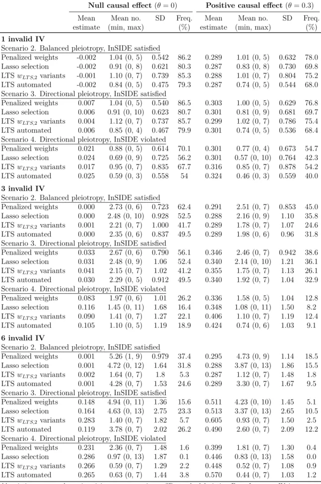
study for Scenarios 1-4 with a null or positive causal effect. . . 68 3.8 Summary statistics on the number of genetic variants penalized or not
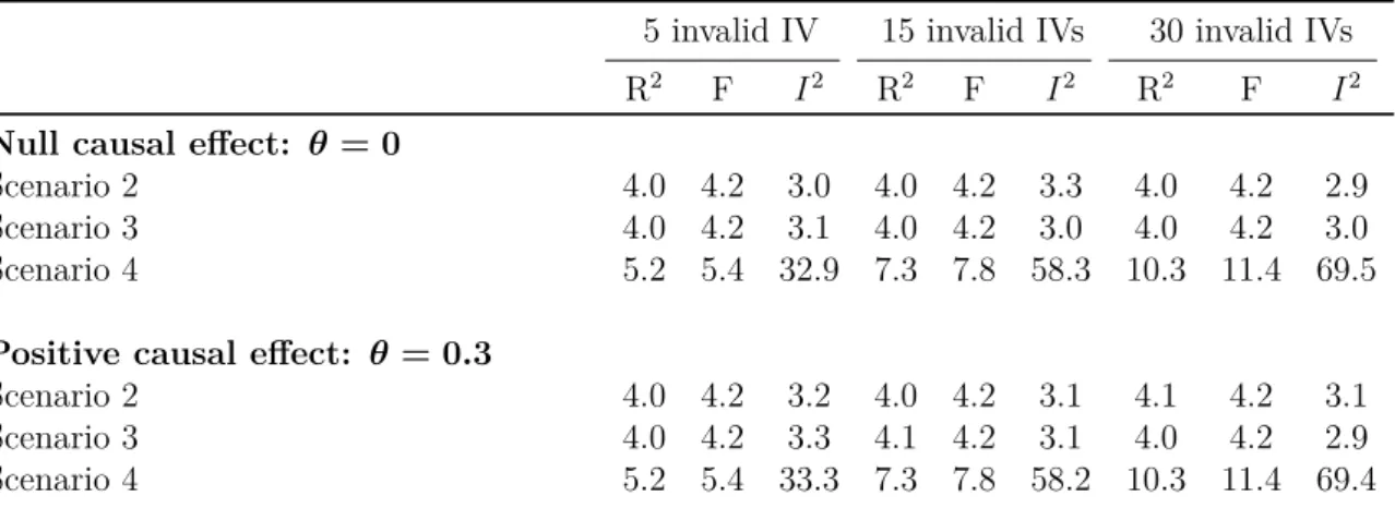
selected in the simulation study for Scenarios 2-4 with a null or positive causal effect. . . 70 3.9 Mean values of the R2 (%), F-statistic and I2 (%) when the simulation
study was re-performed for 100 genetic variants. . . 71 3.10 Results from the simulation study for Scenarios 2-4 when the number of
genetic variants was increased to 100 for a null causal effect. . . 73 3.11 Results from the simulation study for Scenarios 2-4 when the number of
3.12 Summary statistics on instrument strength and prevalence of the out-come from the simulation study for Scenarios 1-4 with a null or positive causal effect and binary outcome. . . 76 3.13 Results from the simulation study with a binary outcome for Scenario 1
with a null or positive causal effect. . . 77 3.14 Results from the simulation study for Scenarios 2-4 with a null causal
effect and binary outcome. . . 79 3.15 Results from the simulation study for Scenarios 2-4 with a positive
causal effect and binary outcome. . . 80 4.1 Estimates of the approximate log causal odds ratios for coronary heart
disease per unit increase in high-density lipoprotein cholesterol. . . 102 4.2 Estimates of the approximate log causal odds ratios for coronary heart
disease per unit increase in high-density lipoprotein cholesterol, low-density lipoprotein cholesterol, and triglycerides. . . 103 4.3 Summary statistics on instrument strength for a null and positive causal
effect when the genetic associations were generated independently in the simulation study. . . 107 4.4 Summary statistics on instrument strength for a null and positive causal
effect when the genetic associations were correlated in the simulation study. . . 108 4.5 Results from the simulation study for a null and positive causal effect
when the genetic associations were generated independently. . . 110 4.6 Results from the simulation study for a null and positive causal effect
when the genetic associations were correlated. . . 111 4.7 Results from the simulation study for a null and positive causal
ef-fect when the risk factors were causally dependent and the genetic associations were generated independently. . . 116 4.8 Results from the simulation study for a null and positive causal
ef-fect when the risk factors were causally dependent and the genetic associations were correlated. . . 117 5.1 Contingency table for a 2×2 factorial randomized clinical trial. . . 127
5.2 Table comparing the effect of lowering low densty lipoprotein levels on the risk of coronary heart disease by inhibiting different gene regions. . 134 5.3 Number of instrumental variables in the simulation study. . . 147
List of tables xxvii 5.4 Results from the simulation study when there were no cross-over variants
and the directly generated risk factors were used. . . 149 5.5 Results from the simulation study when there were no cross-over variants
and the mean centred risk factors were used. . . 150 5.6 Mean number of pariticpants in each cell of the 2×2 contingency table
for the simulation study. . . 151 5.7 Results from the simulation study when there were cross-over variants
and the mean centred risk factors were used. . . 152 5.8 Results from the simulation study when there were no cross-over variants
and the directly generated risk factors were used by the amount of variance the genetic variants explained in the risk factors. . . 155 5.9 Results from the simulation study when there were five cross-over
vari-ants and the directly generated risk factors were used by the amount of variance the genetic variants explained in the risk factors. . . 156 5.10 Results from the simulation study when there were eight cross-over
variants and the directly generated risk factors were used by the amount of variance the genetic variants explained in the risk factors. . . 157 5.11 Results from the simulation study when the directly generated risk
factors were used by the amount of variance the genetic variants explained in the risk factors and by the number of cross-over variants. . . 158 5.12 Results from the simulation study using summary level data when there
were five cross-over variants. . . 163 5.13 Mean number of particiapants in each cell of the 2×2 contingency table
from the simulation study when the gene scores were dictohomized. . . 169 5.14 Results from the simulation study when the gene scores were treated as
continous and binary variables. . . 171 5.15 Summary statistics of body mass index, alcohol consumption and systolic
blood pressure by gene score classification. . . 175 5.16 F-statistic and Sanderson-Windmeijer conditional F-statistic for body
mass index, alcohol consumption and the product of body mass index and alcohol consumption. . . 176 5.17 Estimates of the interaction effect of body mass index and alcohol
consumption on systolic blood pressure. . . 177 6.1 Information on the traits associated with the genetic variants considered
6.2 Summary of the demographic characteristics of the UK Biobank partici-pants included in the analysis. . . 207 6.3 Summary statistics of the adiposity and body composition measurements
from UK Biobank. . . 208 6.4 Summary statistics relating to asthma status from UK Biobank. . . 209 6.5 Summary statistics on forced vital capacity and forced expiratory volume
from UK Biobank. . . 209 6.6 Summary statistics on instrument strength for body composition
mea-surements in UK Biobank. . . 210 6.7 Estimates of the approximate causal log odds ratios for ever diagnosis
of asthma per unit increase in body mass index from UK Biobank. . . . 215 6.8 Estimates of the approximate causal log odds ratios for current asthma
per unit increase in body mass index from UK Biobank. . . 218 6.9 Estimates of the approximate causal log odds ratios for asthma per unit
increase in body mass index using summary level data. . . 226 H.1 Number of robust regression models that failed to report a standard
error in the simulation study. . . 407 H.2 Results from the simulation study when an intercept term was included
in the robust regression, penalized weights, and robust regression and penalized weights methods for a null and positive causal effect. . . 409 H.3 Results from the simulation study when the data was generated for a
one-sample Mendelian randomization study and a null causal effect. . . 411 H.4 Results from the simulation study when the data was generated for a
one-sample Mendelian randomization study and a positive causal effect. 412 I.1 Information on the genetic variants considered for the Mendelian
ran-domization analysis using the UK Biobank dataset. . . 417 I.2 Estimtes of the genetic associations with body mass index from UK
Biobank. . . 420 I.3 Estimtes of the genetic associations with bioelectrical impedance analysis
measurements for fat mass index from UK Biobank. . . 423 I.4 Estimtes of the genetic associations with bioelectrical impedance analysis
measurements for fat-free mass index from UK Biobank. . . 425 I.5 Estimtes of the genetic associations with dual-energy X-ray
List of tables xxix I.6 Estimtes of the genetic associations with dual-energy X-ray
measure-ments for fat-free mass index from UK Biobank. . . 429 I.7 Estimtes of the genetic associations with asthma from UK Biobank. . . 431 I.8 Estimates of the genetic associations with asthma extracted from the
GABRIEL consortium. . . 434 I.9 Estimates of the genetic associations with body mass index, fat mass
index and fat-free mass index from the UK Biobank dataset for the proxy genetic variants. . . 435
Chapter 1
Introduction
Epidemiology investigates the determinants of health outcomes and the distribution of diseases at the population level. Epidemiological research can inform disease aetiology, the effectiveness of treatments on disease outcomes, public health policies, and the prioritization of healthcare resources. To strengthen the credibility of these findings and recommendations, epidemiology must consider questions of cause and effect.
In this Chapter, we discuss what is meant by the causal effect of a risk factor on an outcome (Section 1.1), and consider the detection and estimation of these effects in randomized clinical trials (Section 1.2), epidemiological studies with observational data (Section 1.3), instrumental variable analyses (Section 1.4), and finally, Mendelian randomization (Section 1.5). We then provide motivation for the work presented (Section 1.6), and outline the structure of the dissertation (Section 1.7).
1.1
Causal effect
In this dissertation, we consider a causal effect to be a measure of the impact an intervention on the risk factor X has on the distribution of an outcomeY. We use the
notation do(X =x) introduced by Pearl [1] to illustrate that X has been intervened
on and set to the value x. If the risk factor has a causal effect on the outcome, then an
intervention on X will change the distribution of Y, and the conditional distribution p(Y =y|do(X =x)) will be dependent on the valuex.
An observational association considers differences in the outcome when the risk factor is observed at different values. If the risk factor is associated with other variables, such as variables that confound the association betweenXandY, then the observational
association of the risk factor on the outcome may highlight differences in the risk factor and the confounders. Hence, the conditional distribution p(Y =y|X = x) may not
be equivalent to p(Y =y|do(X =x)) [2]. This distinction between an observational
association and a causal effect has contributed to the phrase ‘correlation does not imply causation’.
1.2
Randomized clinical trials
Randomized clinical trials (RCT) are considered the ‘gold standard’ of assessing the effectiveness of a treatment on a disease outcome [3]. In its simplest form, a RCT randomly allocates participants to receive the treatment or control (no treatment). By randomizing participants to treatment, all known and unknown confounders should be balanced between the two treatment groups [4]. It can be inferred that the treatment has a causal effect on the outcome if the frequency of the disease outcome differs between the randomized groups. RCTs usually perform an intention to treat (ITT) analysis where the effect of randomization on the outcome is estimated [5]. The estimate from a ITT analysis will be equivalent to the causal parameter of the average treatment effect (ATE) if all of the participants take the treatment they have been randomly allocated to (‘full compliance to randomization’) [6].
1.3
Epidemiological studies
Due to cost, time, and ethical reasons, it may not be feasible to conduct a RCT to investigate the causal effect of a treatment or modifiable risk factor on a disease outcome [7]. Observational data is often used to investigate the effect of a risk factor on a disease outcome when a RCT cannot be performed. Whilst it is theoretically possible to adjust for the confounders of the risk factor–outcome association in the statistical analysis of the observational data, we cannot guarantee that all of the confounders will have been accounted for (known as ‘residual confounding’) [8]. Observational studies may also be affected by ‘reverse causation’ in which the observed association between the risk factor and outcome is due to a causal effect of the outcome on the risk factor [8].
Due to residual confounding and reverse causation, analyses using observational data that adjust for potential confounders in the statistical model cannot distinguish between correlation and causation. This limitation has led to numerous examples where an apparent association has been identified using observational data, but the result has not been replicated in a RCT. For example, epidemiological studies using observational data suggested that vitamin C has a protective effect against cardiovascular disease
1.4 Instrumental variable analyses 3 [9, 10], but this result was not supported in a RCT where a null effect was reported [11].
1.4
Instrumental variable analyses
Using observational data, an instrumental variable (IV) can be used to infer a causal effect between a risk factor X and an outcome Y. IVs have been applied to a wide
range of research areas, including economics and medical research. For a variable G to
be a valid IV, the following conditions must be satisfied: • IV1: G is associated with the risk factor (G̸⊥⊥X);
• IV2: Gis (marginally) independent of all unmeasured confounders U of the risk
factor–outcome association (G⊥⊥U); and
• IV3: G is independent of the outcome conditional on the risk factor and
con-founders (G⊥⊥Y|(X, U)) [2, 12].
Under the IV1 assumption, there will be a systematic difference in the average levels of the risk factor between the subgroups of G, and the IV2 assumption ensures that
the unmeasured confounders U will be equally distributed between these subgroups.
The IV3 assumption guarantees that Gonly has an effect on Y viaX, i.e. Gdoes not
have a direct effect on Y.
Figure 1.1 is a directed acyclic graph (DAG) of the variables G, X, Y and U,
where G satisfies the IV assumptions. A DAG is a graphical model that provides a
non-parametric representation of the relationships between a set of variables. In a DAG, nodes are used to represent variables, and these nodes are connected by directed edges, usually represented as single headed arrows. For example, A → B implies that the
variableA has a direct effect on variableB. Conversely, if two nodes are not connected
by an arrow, this infers that there is no direct effect between the two variables. A DAG must not contain a variable C which has a sequence of directed edges that lead back
to C. Hence, a DAG cannot have any complete cycles. DAGs do not have to contain
all intermediate variables, such as C in A → C → B, and a node may represent a
collection of variables.
In Figure 1.1, the IV1 assumption is satisfied by the arrow connecting G to the
risk factor X. IV2 is satisfied as there is no arrow that directly links G and the set of
unmeasured confounders U, and there is no pathway betweenG andU. Finally, IV3 is
𝐺
𝑋
𝑌
𝑈
Fig. 1.1 Directed acyclic graph illustrating the instrumental variable assumptions for the variableGto investigate the causal effect of a risk factor X on a outcome Y, whereU are the set of unmeasured confounding variables of theX−Y association.
DAGs imply that there is a direction of effect between variables, but these effects are not necessarily causal. From Figure 1.1, the joint distribution of Y, X, U and G
can be factorized as:
p(y, x, u, g) =p(y|u, x)p(x|u, g)p(u)p(g), (1.1)
and the DAG will have a causal interpretation with respect to X if we can intervene
on X without changing the distributionsp(y|u, x), p(u) and p(g) in Equation 1.1 [13].
These three distributions should be the same regardless of whether X is set to x′ (i.e. do(X =x′)) or x′ is observed. Sheehan and Didelez [13] refer to this condition as the
‘structural assumption’, and this assumption, along with the three IV conditions, must be satisfied for the DAG in Figure 1.1 to have a causal interpretation with respect to
X. Under this structural assumption, we can express the joint distribution of Y,X, U
and G as:
p(y, u, g|do(X=x′)) = p(y|u, x′)p(u)p(g). (1.2)
In Section 2.1, we consider how an IV can be used to statistically test for a causal effect betweenX and Y within the context of Mendelian randomization. We define
the additional assumptions required to produce a point estimate of the causal effect (Section 2.2), and outline the methods commonly used in the IV literature to estimate
the causal effect (Section 2.3).
1.5
Mendelian randomization
Mendelian randomization uses genetic variants as IVs to detect and/or estimate the causal effect of a risk factor on an outcome using observational data. Katan [14] first introduced the idea of using genetic variants as IVs to detect causal effects, and their use in epidemiological research has been popularized by Davey Smith and Ebrahim [15].
1.5 Mendelian randomization 5 In this Section, we discuss the merits of using genetic variants as IVs and introduce different types of Mendelian randomization studies.
1.5.1
Using genetic variants as instrumental variables
A genetic variant must be associated with the risk factor for the IV1 assumption to be satisfied. Since there has been a substantial increase in the number of genome wide association studies (GWAS), and the results from these studies are usually publicly available, this assumption should be relatively straight forward to verify. Typically, uncorrelated genetic variants (not in linkage disequilibrium) that are associated with the risk factor at the genome wide significance level (p-value<5×10⁻⁸) are considered
in a Mendelian randomization study.
Since increases in sample sizes have led to more genetic variants being identified in GWASs, and common genetic variants typically explain little variation in the risk factor, many Mendelian randomization analyses now include multiple genetic variants as IVs [16]. The genetic variants do not have to be causally associated with the risk factor to be valid IVs. Any genetic variant that is in linkage disequilibrium with the causal variant and satisfies the IV assumptions can be used as a IV [17]. Including multiple genetic variants in the analysis will only increase the power to detect the causal effect if the variants explain additional variability in the risk factor [18, 19]. Note that since genetic variants are determined at conception, the association between the variant and the risk factor should not be subject to reverse causation [20, 21].
The IV2 assumption that the genetic variant is not associated with any of the un-measured confounders of the risk factor–outcome association is an untestable condition. The assumption that genetic variants are ‘randomly’ distributed in the population, combined with Mendel’s laws of inheritance, are often used to justify the validity of the IV2 assumption as it implies that the genetic variants are randomly distributed in the population with respect to potentially confounding variables, such as social and environmental factors [15]. The credibility of the IV2 condition could be considered by testing the genetic variants with known measured confounders of the risk factor– outcome association in the dataset used in the main analysis, and by looking up the genetic associations with known unmeasured confounders in external datasets and consortia. Although this is a sensible suggestion, it is by no means exhaustive.
If a genetic variant is associated with more than one trait then it is said to be a ‘pleiotropic’ variant. The inclusion of a pleiotropic genetic variant in a Mendelian randomization analysis may lead to the violation of the IV2 or IV3 assumptions. Since GWASs have identified many genetic variants that are associated with multiple traits,
including pleiotropic variants in a Mendelian randomization study is a major concern [22]. This limitation has led to various methods being introduced into the Mendelian randomization literature that either detect and remove pleiotropic variants, or estimate consistent causal effects in the presence of pleiotropic variants.
1.5.2
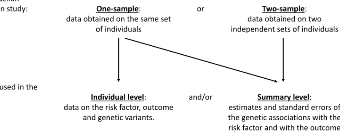
Classification of studies
Figure 1.2 provides an illustration of the two main types of Mendelian randomization studies considered in the literature and this dissertation, and the type of data that can be used in the analysis of these two studies. When Mendelian randomization was initially considered in the literature, data on the same set of individuals was generally used, known as a ‘one–sample’ Mendelian randomization study [23]. Typically, individual level data on the risk factor, outcome, and genetic variants are used in the analysis model for one–sample Mendelian randomization. However, it is possible for estimates and standard errors of the genetic associations with the risk factor and with the outcome, referred to as ‘summary level data’, to be used in the analysis of a one–sample Mendelian randomization study.
It has now become increasingly popular for Mendelian randomization analyses to use data from two independent samples, known as a ‘two–sample’ Mendelian randomization study [24]. Two–sample Mendelian randomization studies generally use summary level data where the estimates and standard errors of the genetic associations with the risk factor are obtained from one sample, and the estimates and standard errors of the genetic associations with the outcome are obtained from the other sample. It is assumed that the two independent samples come from the same underlying population.
Typically, ‘summary level data’ refers to the case where the genetic associations with the risk factor and the genetic associations with the outcome have been estimated in two independent samples (i.e. a two–sample Mendelian randomization study). However, as noted above, it is possible for summary level data to be used in a one–sample study. Throughout this dissertation, we assume that ‘summary level data’ refers to the two–sample setting unless explicitly stated otherwise.
Since access to individual level data can be restrictive, and summary level data is often publicly available from GWASs and large consortia, two–sample Mendelian randomization studies continue to grow in popularity [25]. This has led to numerous methodological developments in using summary level data in Mendelian randomization. Databases, such as Phenoscanner [26], and software, such as MR-Base [27], have been developed to allow users to extract summary level data from published GWASs and
1.6 Motivation for the dissertation 7 Type of Mendelian
randomization study: One-sample:
data obtained on the same set of individuals
or Two-sample: data obtained on two independent sets of individuals
Type of data used in the
analysis: Individual level: data on the risk factor, outcome
and genetic variants.
and/or Summary level: estimates and standard errors of the genetic associations with the risk factor and with the outcome Fig. 1.2 Diagram illustrating some of the types of Mendelian randomization studies and the data used in the analysis.
consortia databases. MR-Base will even perform a two-sample Mendelian randomization analysis if the user specifies a risk factor and outcome.
1.6
Motivation for the dissertation
The overarching aim for this dissertation was to develop methods for applied Mendelian randomization studies. Some of the method development in this dissertation has been motivated by our main applied example of investigating the effect of adiposity and body composition on asthma using data from UK Biobank in a one–sample Mendelian randomization study. UK Biobank is a prospective, population based cohort consisting of approximately 500,000 participants aged between 40-69 years living in the UK. Extensive baseline characteristics were collected at recruitment, including adiposity, body composition measurements and genetic information.
The primary research question for this applied example was to use body mass index (BMI) as a measure of adiposity to perform a Mendelian randomization study to investigate the effect of BMI on asthma. Since the results from a Mendelian randomization study may be invalid if the IV2 or IV3 assumptions are violated, we consulted the literature on Mendelian randomization to identify methods that detect or account for the inclusion of pleiotropic variants (discussed in Chapter 2). Identifying gaps in the literature, we developed and extended ‘robust methods’ that downweight or remove pleiotropic genetic variants (Chapter 3). It was anticipated that these methods would be used in the sensitivity analysis for the Mendelian randomization study on BMI and asthma (Chapter 6).
UK Biobank has measurements on body composition, including fat mass (FM) and fat-free mass (FFM). To have a more comprehensive appreciation for the effect of adiposity and body composition on asthma, we considered the possibility of investigating the simultaneous effect of FM and FFM on asthma in a one–sample Mendelian randomization study. Since there is a substantial overlap in the genetic variants that are associated with FM and FFM, the IV assumptions would have been violated if the effect of FM and FFM on asthma had been considered in separate Mendelian randomization analyses. However, multivariable Mendelian randomization has been developed to allow for causal effects of multiple risk factors that share common genetic predictors to be estimated in the same analysis [28].
The estimates from multivariable Mendelian randomization may be invalid if pleiotropic variants that are associated with traits that do not lie on the causal pathways between the risk factors and outcome (violation of the IV3 assumption for multivariable Mendelian randomization) are included in the analysis. However, there are no methods that estimate consistent causal effects of multiple risk factors when pleiotropic variants that violate the IV3 assumption for multivariable Mendelian randomization are included in the analysis. Since the MR-Egger method has been developed to estimate consistent causal effects in the presence of pleiotropic variants when one risk factor is included in the analysis [29], we considered the extension of this method to the multivariable setting (Chapter 4) with the anticipation of using the method in the sensitivity analysis for investigating the effect of FM and FFM on asthma (Chapter 6).
Whilst expanding MR-Egger to the multivariable setting, it became evident that there may be circumstances where detecting interaction effects between risk factors would be of interest. This observation initiated work on estimating statistical interac-tion effects in ‘factorial’ Mendelian randomizainterac-tion (Chapter 5). The methodological framework required to estimate interaction effects between risk factors in Mendelian randomization has not been considered in the literature. However, there has been ap-plied examples on estimating interaction effects between pharmacological interventions, but there remain various unresolved methodological issues relating to this application. Note that this work was not directly relevant to our investigation of the effect of adiposity and body composition on asthma as we did not suspect that there would be statistical interactions in this applied project.
In the next Section, we provide an overview of the dissertation and outline the material presented in each Chapter.
1.7 Structure of the dissertation 9
1.7
Structure of the dissertation
The additional assumptions required to estimate causal effects and the most frequently used IV methodology in Mendelian randomization are outlined in Chapter 2. The difficulties of considering binary outcomes in Mendelian randomization are highlighted and discussed in this Chapter. Chapter 2 also contains a literature review on sensitivity analyses in Mendelian randomization that try to identify or account for pleiotropic genetic variants to produce unbiased causal estimates. The review focuses on methods that use summary level data of the genetic associations with the risk factor and with the outcome in Mendelian randomization.
Chapter 3 introduces four robust methods for Mendelian randomization using summary level data. In this Chapter, we assume that heterogeneity among the causal ratio estimates is due to pleiotropic variants. As such, the proposed methods in Chapter 3 remove or downweight the contribution of genetic variants with heterogeneous causal ratio estimates. These methods are compared to other methods in the literature (outlined in Chapter 2) in two applied examples and an extensive simulation study. As highlighted in the acknowledgements, this work is adapted and extended on material uploaded to arXiv by Burgess et al. [30] (see Appendix A for a copy of this work). A paper has now been published on this material [31] (see Appendices B and C for a copy of the manuscript and its appendix).
In Chapter 4, we extend the MR-Egger method [29] to the multivariable setting to account for both measured and unmeasured pleiotropy (the ‘multivariable MR-Egger method’). Through theoretical arguments, we outline the assumptions required to obtain a consistent causal estimate from the multivariable MR-Egger method. We apply the method to published genetic data, and consider the performance of the method in a simulation study. A paper has already been published on this material [32] (see Appendices D and E for a copy of the manuscript and its appendix).
Chapter 5 presents work on estimating causal interaction effects of risk factors on an outcome in Mendelian randomization analyses. This extension to the Mendelian randomization framework is considered in a simulation study and an applied example. Interaction effects between pharmacological interventions in Mendelian randomization has already been considered in the literature [33–35], and Chapter 5 also addresses some of the unresolved methodological issues relating to this work. A paper has now been published on this material [36] (see Appendices F and G for a copy of the manuscript and its appendix).
Chapter 6 investigates the causal effect of adiposity and body composition on asthma using data from UK Biobank in an extensive one–sample Mendelian randomization
study. A two–sample Mendelian randomization study is also considered by using data from UK Biobank and the GABRIEL (A Multidisciplinary Study to Identify the Genetic and Environmental Causes of Asthma in the European Community) Consortium [37]. Various Mendelian randomization methodology, including the multivariable MR-Egger method developed in Chapter 4, were considered in the studies.
Finally, Chapter 7 discusses the dissertation as a whole, outlines the limitations of the work, and suggests avenues of further research.
Chapter 2
Statistical methods for Mendelian
randomization
In this Chapter, we outline the sufficient assumptions required to statistically test for and estimate a causal effect (Sections 2.1 and 2.2), introduce the most commonly used IV methods in Mendelian randomization, and highlight some of the issues of estimating the causal effect with a binary outcome (Section 2.3). We define pleiotropic genetic variants within the context of Mendelian randomization and discuss the impact they may have on the causal estimate (Section 2.4). We also discuss heterogeneous ratio estimates and the exploratory analyses typically performed in Mendelian randomization to detect pleiotropic genetic variants (Section 2.5). Finally, we provide an overview of methods that detect or account for pleiotropic variants using summary level data (Section 2.6).
2.1
Testing for a causal effect
We assume that the genetic variant G satisfies the IV assumptions for a risk factor X
and outcomeY. Under the structural assumption (Equation 1.2) in Section 1.4, we can
test for a causal effect of X on Y by testing for an association between G andY. If G
is associated with Y, we can infer that the risk factor is causally associated with the
outcome [2]. If Y ⊥⊥X|U (i.e. there is no arrow between X and Y in Figure 1.1), then
the causal effect between X and Y is zero, andG⊥⊥Y. However, the converse does
not always hold, i.e. if G⊥⊥Y it does not necessarily imply that Y ⊥⊥X|U; known as
the ‘non faithfulness’ of a DAG [2].
IfY is a continuous variable, we could regress Y againstG in a linear regression
coefficient will not have a meaningful interpretation and should only be used as a test for a causal effect. We must make additional assumptions to estimate a causal parameter for the effect of X onY (considered in Section 2.2 below).
2.2
Additional assumptions for a point estimate
Additional modelling assumptions must be made to estimate the causal effect of the risk factor on the outcome. We consider the scenario where we have a continuous risk factorX, continuous outcome Y, unmeasured confounding variables U of the X−Y
association, and J independent (not in linkage disequilibrium) genetic variants Gj
(j = 1, . . . , J) that satisfy the IV assumptions.
We assume that for each individual i (i= 1, . . . , N1) the risk factor Xi is a linear
function of the J genetic variants Gij (j = 1, . . . , J), the unmeasured confounders Ui
of the X−Y association, and the error term ϵXi:
Xi =β0+ J X j=1
βXjGij+ζXUi+ϵXi,
where βXj is the effect of the jth genetic variant on X, and ζX is the effect of the
unmeasured confounders U on X. Gij is the number of minor alleles at thejth genetic
variant for theithindividual, and can take the value 0, 1 or 2. TheJ genetic associations
with the risk factor βXj (j = 1, . . . , J) can be estimated by regressing the risk factor
against each of the genetic variants in linear regression models, where it is assumed that the minor allele has an additive effect on X. We also assume that for each individual i
(i= 1, . . . , N2) the outcome is a linear function of the risk factorXi, the unmeasured
confounders Ui of the X−Y association, and the error term ϵY i:
Yi =θ0+θXi+ζYUi +ϵY i, (2.1)
where ζY is the effect of the unmeasured confounders U on Y, and θ represents the
causal parameter of interest. Under the structural assumption (Equation 1.2), we assume that Equation 2.1 is valid when X is intervened on or observed. Under these
model assumptions, the causal parameter is given by:
θ= cov(Y, Gj)
cov(X, Gj)
2.3 Estimating the causal effect 13 and this can be estimated by the Wald (ratio) estimator defined in Section 2.3.1. Note that the J genetic associations with the outcome βYj (j = 1, . . . , J) can be estimated
by regressing the outcome against each of the genetic variants in linear regression models.
Figure 2.1 contains a DAG of Gj, X, U and Y, where Gj satisfies the IV
assump-tions. As highlighted in Section 1.5.1, the arrow between Gj and X does not have to
be causal, but Gj should be in linkage disequilibrium with the genetic variant that
has a causal effect on X. In Figure 2.1, we have included the parameters defined in
the model assumptions, i.e. θ represents the causal parameter of interest as defined in
Equation 2.2. Strictly speaking, DAGs should provide a non-parametric representation of the relationships between a set of variables, but throughout this dissertation we include the parameters considered in the model assumptions for ease of interpretation.
𝐺" 𝑋 𝑌
𝛽&' 𝜃
𝑈
𝜁& 𝜁+
Fig. 2.1 Directed acyclic graph illustrating the Mendelian randomization assumptions for the J genetic variantsGj (j= 1, . . . , J) to investigate the causal effect of a continuous risk factor
X on a continuous outcomeY. The genetic effect of Gj on X isβXj, and the causal effect of
the risk factor X on the outcomeY isθ. U represents the set of unmeasured variables that confound the association betweenX and Y with effects ζX and ζY.
2.3
Estimating the causal effect
Under the model assumptions defined in Section 2.2, we consider the IV methods that are most frequently used in Mendelian randomization to estimate the causal parameter θ in Equation 2.2: the Wald (ratio) estimator that typically uses summary
level data (Section 2.3.1) [2]; and two stage-least squares (TSLS) regression that uses individual level data (Section 2.3.1) [38]. Since this dissertation is primarily interested in Mendelian randomization methods that use summary level data, the Wald (ratio) estimator is discussed in detail. Although not considered here, methods based on limited information maximum likelihood [39], generalised methods of moments [40, 41], and Bayesian approaches [42, 43] may also be used to estimate the causal effect. Since
we assume that Y is a continuous variable throughout this Chapter, we highlight some
of the issues of estimating the causal effect when the outcome is binary (Section 2.3.3).
2.3.1
Wald (ratio) estimator
We assume that we have summary level data on the risk factor and outcome from two independent samples: the genetic association estimates ( ˆβXj and ˆβYj) and their
standard errors (se( ˆβXj) and se( ˆβYj)) for the J genetic variantsGj (j = 1, . . . , J). The
causal effectθ of the risk factorX on the outcome Y can be estimated with one genetic
variant Gj using the Wald (ratio) method by dividing the genetic association estimate
with the outcome by the genetic association estimate with the risk factor: ˆ
θj = βˆYj
ˆ
βXj
. (2.3)
The ratio method can also be applied directly to individual level data. For example, if
Gj consisted of two subgroups, then the ratio estimator is the average difference in the
risk factor between the two subgroups ofGj divided by the average difference in the
outcome between the two subgroups of Gj.
An estimate of the causal effect based on all the genetic variants can also be obtained from the weighted average of the J causal ratio estimates:
ˆ θIV W = PJ j=1wjθˆj PJ j=1wj , (2.4)
wherewj is the inverse-variance of the causal ratio estimate ˆθj [44]. The pooled estimate
in Equation 2.4 is known as the ‘inverse-variance weighted’ (IVW) method [45]. Under a fixed effect model, where we assume that there is no heterogeneity among the causal ratio estimates [46], the variance of the IVW estimate is given by:
var(ˆθIV W) =
1
PJ j=1wj
. (2.5)
The inverse-variance weightswj in Equations 2.4 and 2.5 can be approximated from
a delta method expansion of the ratio estimate [47]. The first order approximation of
wj from the delta expansion is most commonly used in the IVW estimator [48]:
1st order approximation of w j = ˆ βX2j se( ˆβYj)2 . (2.6)
2.3 Estimating the causal effect 15 Equation 2.6 assumes that there is no uncertainty in the genetic associations with the risk factor, known as the NO Measurement Error (NOME) assumption [49]. The NOME assumption will only be satisfied if N1 is infinite. Since summary level data
is obtained from GWASs and consortia with very large sample sizes, the NOME assumption may be considered reasonable.
The causal effect of the risk factor on the outcome can also be estimated using a weighted linear regression of the genetic association estimates with the risk factor ( ˆβXj) and the genetic association estimates with the outcome ( ˆβYj) [45], with the
inverse-variance as weights (se( ˆβYj)
−2): ˆ βYj =θIV WβXˆ j+ϵj, ϵj ∼ N(0, φ 2se( ˆβY j) 2), (2.7)
where ϵj represents the error term, φ represents the residual standard error, and the
intercept term is set to zero under the IV2 and IV3 assumptions. To obtain the same variance as the IVW estimate in Equation 2.5, the residual standard error in the weighted linear regression model in Equation 2.7 must be set to one. By fixingφto one,
Equation 2.7 is equivalent to performing a fixed-effect meta-analysis of the J causal
ratio estimates ˆθj (j = 1, . . . , J) [50].
If heterogeneity among the ratio estimates is suspected, then a multiplicative random-effects model may be preferred to a fixed-effect model. Although the point estimates from the fixed- and random-effect models will be the same, the standard error of the causal estimate from the multiplicative random-effects model will be larger if there is heterogeneity among the ratio estimates. The variance of the IVW estimator under a multiplicative random-effect model with first order weights (Equation 2.6) is given by: var(ˆθIV W) = ˆ φ2 PJ j=1βˆX2jse( ˆβYj) −2 ,
where ˆφ is the estimate of the residual standard error. If ˆφ > 1, then this suggests
that there is over-dispersion in the ratio estimates [50]. Note that it is not biologically plausible for the causal ratio estimates to be under-dispersed (ˆφ <1) if the genetic
variants are independent (not in linkage disequilibrium) [46]. ˆφ is not allowed to be
lower than one to ensure that the causal estimate from the multiplicative random-effect model is never more precise than the estimate from the fixed-effect model.
Instead of using multiplicative random-effects, an additive random-effects model could be used (not considered throughout this dissertation). This would be equivalent
to performing an additive random-effects meta-analysis of the J causal ratio estimates
ˆ
θj (j = 1, . . . , J) [50]. The estimates and standard errors from the fixed-effects and
additive random-effects models will differ if there is heterogeneity among the J causal
ratio estimates ˆθj (j = 1, . . . , J). However, additive random-effects are rarely used
in Mendelian randomization, with multiplicative random-effects generally being used when heterogeneity among the ratio estimates is suspected. This preference may be due to the fixed-effects and multiplicative random-effects models estimating the same point estimate. Additionally, Bowden et al. [51] have cautioned against the use of additive random-effects as weak instruments may be given too much weight under certain scenarios, resulting in more biased estimates of the causal effect under the additive random-effects model than the fixed-effect model.
2.3.2
Two-stage least squares regression
If there is individual level data on the risk factor, outcome, and genetic variants, then the casual effect θ can be estimated using two-stage least squares (TSLS) regression
[38] in a one–sample Mendelian randomization study. Under TSLS regression, θ is
estimated from the two linear regression models: 1) the regression of the risk factor
X against the genetic variants G; and 2) the regression of the outcomeY against the
predicted values of the risk factor ˆX from 1). The coefficient of ˆX in the second stage
regression model is the TSLS estimate of the causal effect θ. If TSLS is performed
manually, the uncertainty in the first stage regression will not have been accounted for, and the causal estimate will be too precise. As such, TSLS regression software should be used to obtain accurate standard errors of the causal estimate. The estimate from the IVW method will be asymptotically equivalent to the estimate from the TSLS method if the genetic variants are uncorrelated [52].
2.3.3
Binary outcomes
Throughout this Section, we only consider linear additive models where the risk factor X and outcome Y are continuous variables. It is likely that the outcome of
interest will be binary in an epidemiological study, and the causal odds ratio will be the preferred measure of association. Odds ratios are a non-collapsible measure of association, meaning that if the odds ratio takes a constant value across the strata of a covariate, the value obtained from the marginal analysis may not be equal to this constant value [53]. Whilst the numerator in Equation 2.3 could be replaced with the estimate of the log odds ratio of the jth genetic variant with the outcome, and the