23
Register Allocation for Software Pipelined
Multidimensional Loops
HONGBO RONG Microsoft Corporation ALBAN DOUILLET Hewlett-Packard Co. and GUANG R. GAO University of DelawareThis article investigates register allocation for software pipelined multidimensional loops where the execution of successive iterations from ann-dimensional loop is overlapped. For single loop software pipelining, the lifetimes of a loop variable in successive iterations of the loop form a repetitive pattern. An effective register allocation method is to represent the pattern as a vector of lifetimes (or a vector lifetime using Rau’s terminology [Rau 1992]) and map it to rotating registers. Unfortunately, the software pipelined schedule of a multidimensional loop is considerably more complex and so are the vector lifetimes in it.
In this article, we develop a way to normalize and represent the vector lifetimes, which captures their complexity, while exposing their regularity that enables a simple solution. The problem is formulated as bin-packing of the multidimensional vector lifetimes on the surface of a space-time cylinder. A metric, called distance, is calculated either conservatively or aggressively to guide the bin-packing process, so that there is no overlapping between any two vector lifetimes, and the register requirement is minimized. This approach subsumes the classical register allocation for software pipelined single loops as a special case. The method has been implemented in the ORC
This article is an extension of the conference paper in Register Allocation for Software Pipelined Multi-dimensional Loops [Rong et al. 2005] which appears in theProceedings of the ACM SIGPLAN 2005 Conference on Programming Language Design and Implementation (PLDI05). This version extends our method to more general loops and schedules, with more theoretical and experimental results; code generation is also illustrated to show how the register allocation results are consumed. Section 6, Section 7.4, Section 9, Appendix A.6 and Appendix B are new sections. There are also significant additions to Section 3, Section 5 and Section 8. Section 7.1 and 7.3 are revised excepts from Rong and Govindarajan [2007] with permission of CRC.
Authors’ addresses: H. Rong, One Microsoft Way, Microsoft Corporation, Redmond WA 98052; email: [email protected]; A. Douillet, Hewlett-Packard Co., Palo Alto, CA 56225; email: [email protected]; G. R. Gao, University of Delaware, Newark, DE 19716; email: [email protected].
Permission to make digital or hard copies of part or all of this work for personal or classroom use is granted without fee provided that copies are not made or distributed for profit or direct commercial advantage and that copies show this notice on the first page or initial screen of a display along with the full citation. Copyrights for components of this work owned by others than ACM must be honored. Abstracting with credit is permitted. To copy otherwise, to republish, to post on servers, to redistribute to lists, or to use any component of this work in other works requires prior specific permission and/or a fee. Permissions may be requested from Publications Dept., ACM, Inc., 2 Penn Plaza, Suite 701, New York, NY 10121-0701 USA, fax+1 (212) 869-0481, or [email protected].
C
2008 ACM 0164-0925/2008/07-ART23 $5.00 DOI 10.1145/1377492.1377498 http://doi.acm. org/10.1145/1377492.1377498
compiler and produced code for the IA-64 architecture. Experimental results show the effectiveness. Several strategies for register allocation are compared and analyzed.
Categories and Subject Descriptors: D.3.4 [Programming Languages]: Processors—Compilers, Optimization
General Terms: Algorithms, Languages
Additional Key Words and Phrases: Software pipelining, register allocation ACM Reference Format:
Rong, H., Douillet, A., and Gao, G. R. 2008. Register allocation for software pipelined multi-dimensional loops. ACM Trans. Program. Lang. Syst. 30, 4, Article 23 (July 2008), 68 pages. DOI= 10.1145/1377492.1377498 http://doi.acm.org/10.1145/1377492.1377498
1. INTRODUCTION
To software pipeline a multidimensional loop (i.e., a loop nest), traditional ap-proaches mainly focus on scheduling of the innermost loop and extend the sched-ule toward an outer loop by hierarchical reduction [Lam 1988; Muthukumar and Doshi 2001; Wang and Gao 1996]. An alternative way is to perform inner-most loop software pipelining after loop transformations [Carr et al. 1996]. The other approaches extend the classical hyperplane scheduling to achieve an opti-mal periodic schedule, assuming an infinite number of resources [Ramanujam 1994; Gao et al. 1993].
Single-dimension Software Pipelining (SSP) [Rong et al. 2007b] directly over-laps the iterations of ann-dimensional (n-D) loop under resource constraints. It simplifies the n-D loop scheduling problem into a 1-D (1-dimensional) loop scheduling problem, produces a 1-D schedule, and maps it back to then-D itera-tion space to generate a parallelized loop nest. The classical modulo scheduling of single loops [Allan et al. 1995] is subsumed by SSP as a special case. SSP is feasible when then-dimensional loop has a rectangular iteration space and contains no sibling inner loops in it. This article investigates register allocation for loop nests software pipelined by SSP.
For single-loop software pipelining, the lifetimes of a loop variable in suc-cessive iterations of the loop form a repetitive pattern. An effective register allocation method is to represent the pattern as a vector of lifetimes (or a vec-tor lifetime using Rau’s terminology [Rau 1992]) and map it to rotating reg-isters [Rau et al. 1992; Dehnert and Towle 1993]. Unfortunately, the software pipelined schedule of a loop nest is considerably more complex and so are the vector lifetimes in it, which leads to interesting and serious challenges for reg-ister allocation, for example, how to represent such vector lifetimes? How close and how far can two vector lifetimes be put together without conflict? How to identify legal and illegal registers for a vector lifetime? And what strategy should we use to minimize the number of allocated registers?
In this article, we develop a way to normalize and represent the vector lifetimes, which captures their complexity and exposes their regularity that enables a simple, yet powerful solution. The problem is formulated as bin-packing of the multidimensional vector lifetimes on the surface of a cylinder– with time as axis and registers as the circle such that there is no overlapping
Fig. 1. A software-pipelined loop.
between the vector lifetimes, and the circumference of the circle is minimized. A metric called distance is developed to guide the bin-packing algorithm to achieve the goal. This approach subsumes the classical register allocation for software pipelined single loops [Rau et al. 1992; Dehnert and Towle 1993] as a special case.
This approach has been implemented in the ORC compiler for Itanium ar-chitecture. Experiments indicate impressive effectiveness of our approach in minimizing the number of allocated registers. Several allocation strategies are compared and analyzed. As the consumer of the register allocation results, code generation is also illustrated.
2. SOFTWARE PIPELINING FOR SINGLE LOOPS
This section briefly reviews a classical software pipelining method and the cor-responding register allocation approach for a software pipelined loop. The code generation process, which happens after register allocation, is introduced later in Section 7.3.
2.1 Software Pipelining
Software pipelining [Allan et al. 1995] exposes instruction-level parallelism by overlapping successive iterations of a loop.Modulo scheduling[Allan et al. 1995; Huff 1993; Intel 2001] is an important and probably the most commonly used approach for software pipelining.
In modulo scheduling, instances of an operation from successive iterations are scheduled with an initiation interval (II) ofT cycles. This is referred to as the modulo property. The schedule length l is defined as the execution time of a single iteration. Then each iteration is composed of S = Tl number of stages with each stage takingT cycles. The schedule consists of three phases: theprologto fill the pipeline, thekernelto be executed multiple times, and the
epilogto drain the pipeline.
A valid modulo schedule respects the dependence constraints and (hard-ware) resource constraints. During scheduling, the resource usage is tracked by a reservation table. Because of the modulo property, a resource is used, repet-itively, everyT cycles. So the reservation table needs only to be as long as the II. It is therefore called aModulo Reservation Table(MRT) [Rau 1994].
Example: Figure 1(a) shows an example intermediate representation of a single loop where a temporary name (TN) represents a variable. We use the no-tation TN{d}to denote a value of the variable definedd iterations before. For
example, TN{1}refers to the TN value defined in the previous loop iteration. When the value is defined in the current iteration (i.e.,d =0), we denote it sim-ply with TN. Figure 1(b) is the corresponding data dependence graph (DDG) of the loop where each node represents an operation, and an edge is a dependence, labeled with the dependence distance vector, which is a 1-dimensional vector in the single-loop case. Suppose the resources are two function units FU1 and FU2, each able to perform any operation, and operationsa,bandchave a unit latency. A nonoptimal modulo schedule is shown in Figure 1(c) with T = 2,
l =6, andS =3. The kernel is highlighted in darker color. After scheduling, the MRT in Figure 1(d) encodes the resource usage. FU1 is assigned operation
aandc, and FU2 operationb. The schedule will be used later to illustrate the register allocation and code generation approaches for software pipelined single loops.
2.2 Register Allocation
We briefly review the classical register allocation for software-pipelined single loops [Rau et al. 1992; Dehnert and Towle 1993] with target architecture sup-port in the form of arotating register file[Rau et al. 1992; Intel 2001], which is a set of physical registers organized in a circle.
A scalar lifetime is the lifetime of a loop variable for a given iteration of the loop. The variable has one operation to produce a value and one or more operations to consume the value. The scalar lifetime starts when the producer is issued and ends when all of the consumers have finished.1 All the scalar lifetimes of the loop variable over all the iterations of the loop compose the
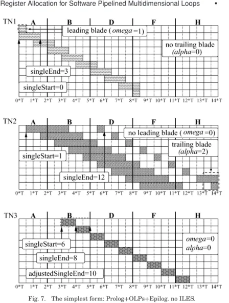
vector lifetime of the loop variable. The vector lifetime can be represented on a space-time diagram where time is on the horizontal axis and the physical registers on the vertical axis. Note that this diagram is flat and assumes an infinite number of physical registers. For example, the space-time diagram for TN1 and TN2 in Figure 1 is shown in Figure 2(a), assuming they are the same class of variables, for example, integer variables.
A vector lifetime is composed of awand(the diagonal band), aleading blade
in case of live-in values, and atrailing bladein case of live-out values. We refer
1This definition is to support interrupt handling in a hardware model where operations, once issued, always go to completion before any interrupt is handled [Rau et al. 1992]. Assume the following two operations are executed at the same time step:a:x = ...andb: ...= y. According to the definition,xis live from this time step, andyis live until operationbis completed. Thusxandy will not be allocated the same register. If during the execution, an interrupt happens, the hardware will automatically reexecute both operations. It can do so because all the input registers still keep the original values, without being overwritten. For example, yis still kept in a register, which is different from that ofx, and is not possible for it to be overwritten byx, even ifxmight have been produced. On the other hand, this definition prevents register coalescing for a copy operation like c:v=u, whereuandvwill be forced to have different registers. In a different hardware model, the definition of the scalar lifetime may be relaxed such that it starts when the producer finishes and ends when the last consumer starts. In this case, register coalescing is feasible. For operation c, the two variablesuandvmay be allocated the same physical register. More specifically, suppose both variables have no live-in or live-out values, then when we introduce the distance calculation in Equation (4) later, the reader will find that D I ST[u,v]= [d3,+∞], whered3 <0, because end(u)<start(v). As 0 is included in this distance,uandvmay be allocated the same register.
Fig. 2. Integer register allocation.
to the scalar lifetime of a loop variable corresponding to the first iteration, that is, iteration 0, as the first scalar lifetime, although it appears after the leading blade. In Figure 2(a), TN2 is made of a wand only. TN1 has a leading blade for it has a live-in value and a trailing blade (assume it has a live-out value).
Correspondingly, a vector lifetime is represented by a 4-tuple (start, end, omega, alpha). The start and end values refer to the start and end cycles of the first scalar lifetime which is taken as a reference due to the repetition of the scalar lifetimes. Then, the scalar lifetime corresponding to iterationistarts at
start+i∗T and ends atend+i∗T. Omega is the number of live-in values for the loop variable. Alpha represents the number of live-out values for the loop variable. For example, the vector lifetimes of TN1 and TN2 are represented as (1, 3, 1, 1) and (0, 6, 0, 0), respectively.
A physical register x is said to be allocated to a vector lifetime v if it is allocated to the first scalar lifetime ofv. Intuitively, register allocation packs the vector lifetimes on the space-time diagram as close as possible without any conflict.Conflictrefers to the fact that two scalar lifetimes that overlap in time are allocated to the same register.
To avoid any conflict, two vector lifetimes must have certain distance between them in the space-time diagram. For two vector lifetimes Aand B, letrA and
rB be the physical registers allocated to Aand B, respectively. The distance
DIST[A,B] is the legal range ofrB−rA, within whichAandBdo not conflict in
the space-time diagram. It must meet the following conditions [Rau et al. 1992]: the wand ofBmust be to the right of the wand of A, and the leading/trailing blades ofBmust be above the leading/trailing blades ofA. Formally,
rB−rA ≥ omega(A) ifomega(B)>0 rB−rA ≥ alpha(A) ifalpha(A)>0 that is, d1 = end(A)−start(B) T (1) d2 = d1 ifomega(B)=0
max(d1,omega(A)) otherwise. (2)
d3 =
d2 ifalpha(A)=0
max(d2,alpha(A)) otherwise.
(3) Then2
DIST[A,B]=[d3,+∞]. (4) For the example in Figure 2(a), DIST[TN2,TN1] = [3,+∞], according to Equations (1)–(4) This can also be seen intuitively from the figure. Similarly, we can calculate thatDIST[TN1,TN2]=[2,+∞].
As implied in the space-time diagram, successive scalar lifetimes of a loop variable will be mapped to consecutive physical registers. However, the rotat-ing register file is cyclic and does not really have infinite number of registers. Therefore, the register allocation on the diagram has to be seen wrapped up as a cylinder with time as the axis and registers as the circle. The circumfer-ence of the circle is the total number of registers required to allocate to the loop. The register allocation problem consists of packing the vector lifetimes on the surface of the cylinder such that there is no conflict, and the circumfer-ence is minimized. An optimal register allocation for the space-time diagram in Figure 2(a) is displayed in Figure 2(b) where TN1 is allocated physical register 0 and TN2 register 2, with a circumference of 5 after the diagram is wrapped into a cylinder.
To achieve such register allocation, the algorithm sorts the vector lifetimes and inserts them one-by-one on the surface of the space-time cylinder without backtracking. Three sorting heuristics can be used [Rau et al. 1992]:start time ordering, where the earliest vector lifetime is inserted first;adjacency ordering, where the vector lifetime to be inserted minimizes the horizontal distance with the previously inserted lifetime; andconflict ordering, which is to vector life-times what graph coloring [Chaitin 2004] is to scalar lifelife-times. The insertion of the chosen lifetime is then decided by one of three strategies:best,first, and
end fits. Best fit finds a register that minimizes the current register usage. First fit chooses the first compatible register starting from register 0, while end fit starts from the register allocated to the vector lifetime inserted at the last step. Note that the register allocation problem can be formulated as a Traveling Salesman Problem (TSP), which is known to be NP-Complete [Rau et al. 1992; Lawler et al. 1985].
2The distance defined in Rau et al. [1992] contains only the lower bound. Here we expand it to a range for clarity.
3. REGISTER ALLOCATION FOR SOFTWARE PIPELINED LOOP NESTS This section briefly motivates and reviews SSP, characterizes the vector life-times in an SSP schedule, formulates the corresponding register allocation problem, and finally proposes key observations to solve it.
3.1 Single-Dimension Software Pipelining
Traditionally, software pipelining is applied to the innermost loop of a given loop nest [Allan et al. 1995; Huff 1993; Rau 1994; Rau and Fisher 1993; Intel 2001] or from the innermost loop to the outer loops hierarchically [Lam 1988; Muthukumar and Doshi 2001; Wang and Gao 1996]. Such an innermost loop-centric approach has several limitations [Rong et al. 2007b]. (1) It commits itself to the innermost loop first without considering how much parallelism the other loop levels have to offer. Software pipelining another loop level might result in higher parallelism. (2) It cannot exploit the data reuse potential in the outer loops. (3) The innermost loop has the highest overhead after software pipelining compared with other loops.3Other software pipelining approaches for loop nests do not consider resource constraints [Ramanujam 1994; Gao et al. 1993].
Software pipelining of a multidimensional loop is proposed to overcome these limitations. It predicts the most profitable loop from the loop nest and chooses it to software pipeline. The challenge is how to handle resource constraints and the multidimensional dependences simultaneously in the context of a single processor. Traditionally, hyperplane scheduling and its extensions [Lamport 1974; Darte and Robert 1994; Ramanujam 1994; Gao et al. 1993] schedule the loop according to the dependences only, assuming infinite resources. These ap-proaches are generally used in the context of large array-like hardware struc-tures (such as systolic arrays). Software pipelining, however, targets only a single processor, which has limited hardware resources. Under the resource constraints, finding the optimal software pipelining schedule of the loop is NP-complete even when the loop is a single loop (the innermost loop). With the multidimensional dependences, the problem is even more challenging.
To address the challenges, we first reduce the n-dimensional scheduling problem into a 1-dimensional scheduling problem, then map the 1-dimensional schedule back to then-dimensional iteration space. More specifically, there are three steps.
(1) Loop selection. A loop in the loop nest is chosen to be software pipelined. This loop, compared with all the other loops in the same loop nest, is predicted to produce the maximum benefit once software pipelined. The benefit can be measured in terms of instruction-level parallelism, data reuse, or any other optimization criteria. Only this loop will be parallelized. Its outer loops, if
3When software pipelining is applied to a loop, the schedule has associated overhead, including initialization, prolog, epilog, and finalization. Such overhead is incurred each time the loop is executed. The overhead is unavoidable no matter what loop transformations have been performed previously. Intuitively, the further out the loop is, the less overhead it has. In a 3-deep loop nest where each loop level is executed 1000 times, the overhead is incurred 1,000,000 times if the innermost loop is pipelined, 1,000 times if the middle loop is pipelined, and 1 time if the outermost loop is pipelined.
any, remain intact. Note that this selected loop may have its own inner loop(s) and thus be a loop nest itself.
(2) 1-D schedule construction. The n-dimensional (n ≥ 1) data-dependence graph of the selected loop is simplified to be 1-dimensional, and based on that, a 1-dimensional schedule is computed, represented by a kernel. No matter how many inner loops the selected loop has, it is scheduled as if it were a single loop. Any traditional modulo scheduling method can be applied to construct this 1-D schedule.
(3) Final schedule computation. Use the 1-D schedule as the building block to construct ann-dimensional parallel loop. This final schedule is semantically equivalent to the selected loop. In theory, this step computes a function that specifies the schedule time of each operation instance. In practice, this step translates into code generation for a target architecture, which will be discussed in Section 7.4.
This approach is referred to as single-dimension software pipelining (SSP) because the problem of multidimensional scheduling is simplified to 1-dimensional scheduling. It is a resource-constrained scheduling method to soft-ware pipeline a loop nest. In contrast to the traditional innermost loop-centric approaches [Lam 1988; Muthukumar and Doshi 2001; Wang and Gao 1996], SSP selects the most profitable loop level from the entire loop nest. It provides the flexibility for any criteria to be used to judge the profitability. It retains the simplicity of the classical modulo scheduling technique for single loops, yet under the same condition can achieve the shortest computation time that could be achieved by traditional innermost-centric approaches. The classical modulo scheduling is subsumed by SSP as a special case. The reader is referred to the scheduling paper Rong et al. [2007b] for details.
Intuitively, in the final schedule, the iterations of the selected loop are issued in parallel, whereas the inner loops within each of the iterations run sequen-tially. LetSnbe the total number of stages corresponding to the innermost loop
in the kernel and T be the initiation interval of the kernel. Every T cycles, an iteration of the selected loop is issued until the processor resources become insufficient to support any new iteration. Then a single group of Sniterations
that are already issued execute their inner loops in parallel. Before this group finishes and frees the resources, all the other iterations stall. Such a stall period is calledInner Loop Execution Segment(ILES).
Example. Figure 3(a) shows the intermediate representation of a double-loop nest. Assume that the outer double-loop is selected by SSP, 3 function units are available, and operations a,b,c,d,ehave latencies of 1, 5, 1, 1, and 1 cycles, respectively. Figure 3(b) shows a possible 1-D schedule (the kernel) constructed. The schedule is not optimal and for illustration purpose only. From this kernel, a final schedule is computed, and the loop nest can be rewritten accordingly as shown in Figure 3(c), whereoi1,i2 refers to the instance of operationo, withi1
as the outer loop index andi2as the inner loop index. An outer loop iteration is issued every T =2 cycles and executes sequentially. The issuing continues until the 10th cycle. From there, no new iterations are issued because otherwise
Fig. 3. A loop nest scheduled by SSP.
there would be resource conflicts between the new and the already running outer loop iterations. Only the first group of iterations continue executing their inner loops. The total number of iterations in a group is equal toSn=3. Once
done, the group drains the pipeline and frees processor resources. In the same time, other outer loop iterations continue to issue and execute. To facilitate understanding, the final schedule in Figure 3(c) is illustrated cycle-by-cycle in Figure 4 where ineffective operation instances are shown in gray color. They
Fig. 5. Generic loop nest scheduled by SSP.
are ineffective because theiri1indexes are beyond the valid range, [0,N1−1]. They are masked from execution using predication as will be illustrated in Section 7.4.
Due to the regular stalls and issuing, repeating patterns naturally appear in the final schedule. The final schedule is composed of a prolog, the repetition of an outer loop pattern (OLP) and an ILES, and an epilog. Each of them consists of multiple copies of the kernel as illustrated in Figure 3(c). In other words, the kernel is the building block of the final schedule.
3.2 Assumptions and Conventions
We assume that a loop nest is composed ofn loops: L1, L2, . . ., Ln, from the
outermost to the innermost level, with each level having exactly one loop as shown in Figure 5(a), whereOPSETx represents a set of nonbranch operations
between the beginnings of two adjacent loops. Each loopLx(1≤x ≤n) has an
index variableixand a trip countNx, whereNx >1. The index is normalized to
change from 0 toNx−1 with unit step. Except for the loop control structures,
there is no branch in the loop nest; branches, if any, have been converted to linear code by if-conversion [Allen et al. 1983].
Since a loop, except the innermost loop, has its own inner loops, it is a loop nest itself. To emphasize this fact, we also refer to a loop as anx-dimensional loop, wherexis 1 plus the total number of inner loops of the loop. For example,
L1is ann-dimensional loop,Lna 1-dimensional loop, etc. A 1-dimensional loop
is also called asingle loop. Sometimes, dimension is also referred to as nesting depth or depth of the loop.
An operation isinloop Lx if it is within the loop body of Lx, including the
inner loops Lx+1,. . .,Ln. An operation isat the loop level of Lx if it is in Lx
but outside of the inner loops. That is, for the current loop nest model, any operation inOPSETx is at the loop level ofLx, and any operation inOPSETx∪
The loop nest has an iteration space. It is a rectangular iteration space if its bounds,N1,N2,. . ., andNn, do not change during the execution of the loop nest,
although they can change before and after it. In this article, the loop that SSP chooses to software pipeline must have a rectangular iteration space. The loop must not have sibling inner loops in it either. This requirement has already been implied by the loop nest model.
Without loss of generality, we assume that SSP selects the outermost loop
L1 for scheduling, and constructs a 1-D schedule, which is represented by a kernel. The stages in the kernel are numbered from right-to-left as 0, 1,. . ., as shown in Figure 5(b). Each stage takes T cycles to execute. If an operation is scheduled at cyclecof stages, where cyclecis relative to the beginning of the stage and 0≤c<T, its 1-D schedule time is equal tos∗T+c.
The 1-D schedule is such that the operations in the same loopLx, including
its inner loops, are scheduled into contiguous stages. The first such stage is referred to as fx, and the last onelx. The total number of stages for loop Lx
is termed Sx, which equalslx− fx+1. If two operations are at different loop
levels, they cannot be scheduled into the same stage. That is, operations at the loop level of Ln are scheduled into stages fn toln; operations at the loop level
of Ln−1are scheduled into stages fn−1toln−1but outside of stages fntoln, etc.
The kernel is such that f1 = 0 ≤ f2 ≤ · · · ≤ fn ≤ ln ≤ ln−1 ≤ · · · ≤ l1. In the current loop nest model, all loops will have the same last stage, that
is,l1 =l2 = · · · =ln. The kernel is then used as a template to build the final
schedule. The general form of the final schedule is shown in Figure 5(c). The loop nest and kernel model just presented are used throughout the article until Section 6 where they will be extended to be more general.
Unless stated otherwise, the term iterationalways refers to an iteration of the outermost loop L1. Aloop variablerefers to a temporary name that has a definition in loopL1, including its inner loops. To be simple, we assume that at each loop level, the variable is either not defined or defined only once. If there are two definitions at the same level, we can conservatively treat the second definition as a use of the first definition. Therefore, for an iteration, we ensure there is either none or only one piece of lifetime defined at each level . This piece of lifetime is formally referred to as anintervalin this article.
Note that the previous assumption does not prevent a loop variable from being defined multiple times, each at a different loop level. Static-Single As-signment (SSA) form [Cytron et al. 1991] is therefore not an assumption in this article. This is because, although our register allocation method can be applied equally to an SSA-formed program, after register allocation, the pro-gram has to be translated out of SSA form. In that process, the φ nodes are translated into parallel copy operations traditionally. However, it is not clear how to translate them correctly in the context of register allocation for soft-ware pipelining as far as we know. Without SSA, we do lose some flexibility: in an iteration, all intervals of the same variable must be allocated to the same register. We leave the register allocation problem under SSA form as a future subject.
The same as the register allocation for software pipelined single loops, a loop variable’s scalar lifetimes are allocated to a set of continuous physical registers.
Fig. 6. The final form of the vector lifetimes.
The registers form a cycle with finite circumference. We assume the registers start from 0. Once a scalar lifetime is allocated a physical register, the value of the scalar lifetime stays in this physical register and never moves to another physical register, that is, the scalar lifetime is never split (moved from one physical register to another). How to apply splitting to reduce register pressure is left as a future subject.
3.3 Features of Vector Lifetimes
Figure 6 shows the space-time diagram for each of the loop variables in our example in Figure 3, corresponding to the final schedule in Figure 4, with seg-ments A through H marked accordingly. They include all the typical features of a vector lifetime in any SSP final schedule.
Similar to the single-loop case, a vector lifetime may have a leading blade when there are live-in values, and a trailing blade when there are live-out values. For example, in Figure 6, TN1 has a leading blade and TN2 a trail-ing blade (assume it has two live-out values). The wand, however, has un-usual features specific to a multidimensional loop due to the following two reasons.
First, an iteration has inner loops within it. This leads to the following features.
(1) Multiple intervals in a scalar lifetime. A variable can be defined and killed multiple times during the execution of an inner loop. See TN2 and TN3 in Figure 6, for example.
(2) Unknown length of an interval at compile time. A variable has an interval live through an inner loop if the variable is live but never redefined, during the execution of this loop. The length of the interval depends on the trip
counts of this loop and its inner loops, which may be unknown at compile time.
Second, an iteration may be stalled and resumed. This leads to two other interesting features.
(3) Stretched intervals. An interval may be stretched longer than usual in the period of an ILES. For example, Figure 4 illustrates the first interval pro-duced by operationband consumed by operationcin each scalar lifetime of TN2 corresponding to iterations 0 to 5. All the intervals have the same length except the two intervals from iterations 3 and 4, which start before but end after the first ILES, segment C.
(4) Delayed initiation of intervals. For example, in Figure 4, the intervals from successive iterations initiate everyT = 2 cycles, except that the interval from iteration 5 is delayed until after the first ILES.
The previous 4 features present novel challenges to register allocation. For-tunately, there is also one useful and important feature.
(5) Repetition of the OLP and ILES segments, as indicated by the general form of a final schedule in Figure 5(c). When an OLP (ILES) repeats, any interval in it repeats as well. This implies that the part of the vector lifetime within an OLP (or ILES) must be identical to that in any other OLP (or ILES). The only exception is that the first and last OLPs and the last ILES may contain a subset of intervals of other OLPs and ILESes due to the ineffective operations at the beginning and the end of the final schedule (see Figure 4). 3.4 Problem Formulation
The problem to be addressed in this article can be formulated as follows: Given a loop nest composed of n loopsL1,L2,. . .,Ln, suppose the outermost loopL1is software pipelined by SSP. Allocate a minimum number of registers to the loop variables, in the presence of the rotating register file. Considering the cyclic structure of a rotating register file, the task is to pack the vector lifetimes on the surface of a cylinder where time is the axis and the number of registers is the circumference such that there is no conflict between any two scalar lifetimes and the circumference is minimized.
3.5 Key Concepts and Intuition
The key to the entire register allocation problem is to efficiently abstract the vector lifetimes, such that their complexity is captured, and their regularity is exposed to enable us to develop a simple solution. Based on the abstract representation of the vector lifetimes, the next key is to accurately measure how close and how far two vector lifetimes can be packed together on the space-time diagram.
We propose a dynamic view of a vector lifetime, which greatly simplifies both lifetime representation and the measurement of the distance between two vector lifetimes. We further propose a conservative and an aggressive way for the measurement.
Fig. 7. The simplest form: Prolog+OLPs+Epilog. no ILES.
3.5.1 The Dynamic View of a Vector Lifetime: the Simplest, Ideal, and Final Forms. A vector lifetime can be viewed in a dynamic way, from its simplest form to its ideal form and eventually to its final form.
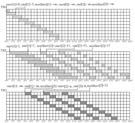
Thesimplest formof a vector lifetime corresponds to the special case where the trip count of any inner loop is imagined to equal 1. The loop nest is then equivalent to a single loop. Therefore it is easy to represent and handle the vector lifetimes using the classical register allocation for software pipelined single loops presented in Section 2.2. For our example, the simplest form of the three vector lifetimes is shown in Figure 7. The simplest form is composed of prolog, OLPs, and epilog but without ILESes.
Theideal formof a vector lifetime corresponds to the ideal case that all the scalar lifetimes are evenly issued everyT cycles. Each iteration runs without stopping as if there were no resource constraint. In this situation, there is no stall in the final schedule. Therefore there are no stretched intervals. The ideal form can be reached by adding to the simplest form the intervals produced
Fig. 8. The ideal form: no stall or resource constraints.
during the execution of the inner loops. The ideal form of the vector lifetimes for our example is shown in Figure 8.
Thefinal formcorresponds to the final schedule, which does have stalls to account for resource constraints. The final form of the vector lifetimes for our example is represented in Figure 6. Every part of a vector lifetime is represented without any omission.
With this dynamic view, it is much easier to mathematically abstract any vector lifetime. First, the simplest form is used to abstract the start and end of the scalar lifetimes. Then the ideal form is used to add the intervals defined at the inner loop levels. Finally, the final form is used for abstraction of the stretched intervals.
Repetition exists in all the three forms. (1) In the simplest and ideal forms, all scalar lifetimes are identical except for the leading and trailing blades. (2) For a scalar lifetime in the ideal form, the interval defined at an inner loop level repeats itself with the sequential execution of this inner loop. (3) In the final form, the ILESes repeat themselves as well, as discussed in Section 3.3.
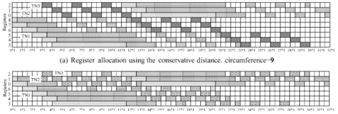
Due to the repetition in representing and handling a vector lifetime, we can simply focus on the first scalar lifetime, the first instance of the interval defined at each inner loop level, and the first ILES and take them as a point of reference. 3.5.2 The Distances Between Two Vector Lifetimes. There are two ways to pack two vector lifetimes on the space-time diagram, one with and the other without interleaving. Figure 9(a) shows a register allocation for our example
Fig. 9. Register allocation examples.
without interleaving. The diagram has already been wrapped around a cylinder. The circumference is 9. Figure 9(b) shows another register allocation where vector lifetimes are interleaved when possible. In this case, the second scalar lifetime of TN3 is interleaved with the first scalar lifetime of TN2, and so on. The interleaving results in a smaller circumference of 7. One may observe that this is an optimal solution; the circumference cannot be further reduced.
Correspondingly, we proposeconservative distanceandaggressive distance, which measure how close and how far in number of registers two vector life-times can be on the space-time diagram without conflict. The conservative dis-tance does not allow for interleaving, whereas the aggressive disdis-tance does. The two distances play a key role in effectively minimizing register usage. The aggressive distance enforces finer control on the selection of a register for a vector lifetime as will be confirmed by our experiments. The three forms of the vector lifetimes will be used appropriately to compute the distances.
4. SOLUTION
Our approach consists of the following steps.
(1) Lifetime normalization. The vector lifetimes are normalized such that any interval has a length known at compile time.
(2) Lifetime representation. The normalized vector lifetimes are abstracted by a set of parameters.
(3) Distance calculation. Using the parameters, a conservative and an aggres-sive distance between any two vector lifetimes, including the distances between a vector lifetime and itself, are computed. Then either the con-servative or the aggressive distance can be used in the following steps. (a) Sorting. The distance is used to order the vector lifetimes.
(b) Bin-packing. The ordered vector lifetimes are inserted one-by-one onto the surface of the space-time cylinder with one of the strategies (best, first, and end fits), respecting the distance between any pair of vector lifetimes. The circumference of the cylinder is assumed to be equal to the maximum number of available registers,R.
Fig. 10. Register allocation algorithm.
(c) Circumference minimization. The last step minimizes the circumfer-ence of the cylinder. The main algorithm is shown in Figure 10. So far, we use a sorting process similar to that in the traditional register allocation for single loops [Rau et al. 1992; Dehnert and Towle 1993] as will be shown in Section 8. However, any other sorting heuristic may also be feasible. The other steps will be presented in detail.
4.1 Lifetime Normalization
An obstacle to lifetime representation is that the length of an interval may be unknown at compile time if it is live through a loop as discussed in Sec-tion 3.3. Without this informaSec-tion, it is impossible to characterize the interval accurately.
In order to represent the vector lifetimes uniformly, we first normalize them such that after normalization any interval has a length known at compile time. To achieve this purpose, any interval that is live through any loop needs to be cut in the middle so that it is not live through the loop any more. Due to the nesting structure of the loops, if the interval is live through any outer loop, it must be live through the innermost one. Therefore, preventing it from being live through the innermost loop is sufficient to prevent it from being live through any other loop. Conceptually, this can be done by inserting a dummy copy instruction TN=TN in the innermost loop where TN is the variable corresponding to the vector lifetime under discussion.
Example: Figure 11(a) shows another example loop nest, where TNx is defined at L1level, live in L2and L3without being redefined. A 1-D schedule is shown in Figure 11(b). Then the first scalar lifetime of TNxin the ideal form would be like that shown in Figure 11(c). The scalar lifetime has a single inter-val, which has indefinite length. The normalization is equivalent to inserting a dummy copy instruction in the innermost loop. Figure 11(d) conceptually illus-trates this effect. Figure 11(e) shows the intervals observed by lifetime repre-sentation in the next step due to the normalization. An interval is highlighted
Fig. 11. Normalize a vector lifetime to simplify the representation.
Fig. 12. Lifetime normalization algorithm.
within a dotted box. The normalization cuts the long interval into repetitive smaller intervals with the execution of the inner loops L3 and L2. We will further study the representation of the intervals later.
Figure 12 shows the algorithm of lifetime normalization. All the references (i.e., definitions and uses) of the variable are gathered into a set, REFS. A reference is expressed as a 4-tuple (time, USE/DEF, omega, level) where time is the 1-D schedule time of the operation that refers to the variable, USE/DEF
indicates whether the reference is a definition or use,omegais 0 if the reference is a definition ord if it is a use that is definedd iterations before, andl evel is the nesting level of the loop that immediately encloses the operation.
If the loop variable is live through the innermost loop Ln, a dummy use
and a dummy definition withtime= fn∗T are added into the references set.
This is equivalent to inserting a copy operation TN=TN at the first cycle of the innermost loop stages in the 1-D schedule, although we never really do such insertion. Inserting the copy instruction at any other cycle of the innermost loop stages is also feasible. Here we choose the first cycle arbitrarily.
4.2 Lifetime Representation
A vector lifetime can be fully abstracted by characterizing its simplest and ideal forms only, with some core parameters. Then the stretched intervals in the final form can be represented by some derived parameters deduced from the core parameters.
4.2.1 Core Parameters: Characterizing the Simplest and Ideal Forms of a Vector Lifetime. First, let us characterize the simplest form in the same way as the traditional register allocation for software pipelined single loops does [Rau et al. 1992] as introduced in Section 2.2. The loop nest is imagined to be a single loop, that is, the trip count of any inner loop is imagined to be 1. SingleStart and singleEnd are the start and end time of the first scalar lifetime. Omega and alpha are the total live-in values and total live-out values, respectively.
Next, we characterize the ideal form. Two elements in a scalar lifetime need to be considered, interval and hole between two adjacent intervals. For the interval defined at a loop level and the hole following it, we represent them by the first instance of the interval and the first instance of the hole in the first scalar lifetime. The representation maximizes the length of the interval, but minimizes that of the hole. This is necessary for two reasons. (1) The definition of the interval may have last uses and successor definitions on different control flow paths due to the multiple back edges of the loop nest. Therefore, the lengths of the interval and the hole may vary. (2) This is required by distance calculation. For example, in calculating the aggressive distance of two vector lifetimes A
and B, an interval of Bis put into a hole of A. If, in the worst case where the interval is the longest possible and the hole is the shortest possible, the hole is still long enough to contain the interval without conflict, then any instances of the interval and the hole would fit without conflict whatever paths are followed by the interval and the hole.
The intervals defined at every loop level and the holes following them are represented by 3 arrays, start, end, and nextStart. For each leveli, we ensure thatend[i]−start[i] is the maximal length of the interval defined at this level, andnext Start[i]−end[i] is the smallest possible size of the hole following it.
Start[i]is the issue time of the definition of the variable at leveli, which is equal to its 1-D schedule time.End[i]is the latest completion time of all possible uses of the definition. There are two special cases: (1) when the definition has no use, end[i] is the completion time of the definition; (2) when there is no
definition of the variable at leveliat all, (start[i],end[i]) are set as (+∞,−∞), indicating that no interval is really defined at this level since the length of the interval isend[i]−start[i]<0. For this reason, the interval will be referred to as aphantom interval. This setting of (start[i],end[i]) naturally enables us to treat the phantom interval the same way as a real interval without any special consideration later in calculating the distances.
NextStart[i]is the earliest issue time of all possible definitions that are fol-lowing this interval in the same iteration.N extstart[i] is naturally defined to be+∞if there is no such definition.
In short, a vector lifetime can be fully represented as a 7-tuple:(singleStart, singleEnd, omega, alpha, start, end, nextStart). The tuple is defined based on the reference setR E F S, which is the output of lifetime normalization. Formal definitions are given in Appendix A.1–A.3.
Example:Figure 7 and 8 show how the vector lifetimes for our example in Figure 6 are characterized in the simplest and ideal forms.
Figure 11(e) shows another example of how the ideal form is described. The variable has no definition at L2 level. So (start[2], end[2])= (+∞,−∞). This phantom interval has a next interval defined at L3 level by operationc (see Figure 11(d)). Thusnextstart[2]=start[3].
For that next interval, its start,start[3], is equal to the issue time of the first instance of operationc. The interval may terminate along three different paths as shown in Figure 11(d). Among the three paths, the second one leads to the longest interval and the third one to the smallest hole. Both paths reach the second instance of operationc. The instance has the latest issue time if it is along the second path and the earliest issue time along the third one, which determineend[3] andnext Start[3], respectively. Note that the hole following the interval has a negative size, that is,next Start[3]−end[3] <0. However, it can be handled in the same way as a normal hole with positive size without any special concern later in calculating the distances.
4.2.2 Derived Parameters: Characterizing the Final Form of a Vector Lifetime. Compared with the simple and ideal forms, the new thing in the final form is the ILESes. The derived parameters describe an ILES, including the stretched intervals appearing there.
The length of a stretched interval cannot be accurately characterized even after lifetime normalization. Unlike the indefinite-length intervals that live through a loop, which can be normalized to have definite lengths by breaking the liveness in the middle of them, stretched intervals are caused by stalls in the final schedule due to limited processor resources, which is unavoidable. For example, the vector lifetimes in Figure 8 are normal, however, the final forms in Figure 6 still have stretched intervals whose lengths remain indefinite at compile time.
Thus, we cannot directly describe a stretched interval horizontally, that is, from the view point of time in its space-time diagram as we did for the scalar lifetimes in the simplest and ideal forms. Fortunately, it is feasible and suffi-cient for register allocation to characterize the stretched intervals vertically, that is, from the viewpoint of space in the space-time diagram. This leads to
the following parameters derived from the core parameters: (outermostInter-valOnly, firstStretch, lastStretch, top, bottom).
The boolean variable outermostIntervalOnlyis true when the loop variable is defined only at the outermost level (after normalization).FirstStretch and
lastStretchare the iteration indexes of the first and last stretched intervals of the variable, respectively, that appear in the first ILES. If there is no stretched interval at all, we set (firstStretch,lastStretch)=(+∞,−∞).
Topis the iteration index of the intervals at the top of the first ILES.Bottom
is one plus the iteration index of the intervals at the bottom of the first ILES. When there is no interval in an ILES, we set (top,bottom)= (+∞,−∞). The differencebottom−toprepresents the vertical thickness of the vector lifetime in an ILES.
As an example, Figure 6 shows the derived parameters of the lifetimes. The formal definitions of the derived parameters are given in the Appendix A.4–A.5. 4.3 Distance Calculation
For any two vector lifetimes Aand B, a metric called distance is used to mea-sure how close and how far Aand Bcan be packed together on the space-time diagram without conflict. There are two types of distances: conservative and aggressive distances.
LetrAandrBbe the registers to be allocated to Aand B, respectively. The
conservative distance, denotedCONS[A,B], (or theaggressive distance, denoted
AGGR[A,B]), defines a legal range ofrB−rAwithin whichAandBdo not
con-flict in the space-time diagram. The conservative distance does not allow the vector lifetimes to interleave, while the aggressive distance does. For conve-nience, letINTL[A,B] be the legal range ofrB−rAwhen the vector lifetimes
interleave, called theinterleaving distance. Then
AGGR[A,B]=CONS[A,B]∪INTL[A,B].
More specifically, for the conservative distance,Bis to the right of any inter-vals of A. For the interleaving distance, an interval of Bis to the right of the corresponding interval of Adefined at the same loop level. For convenience, in either case, we will say that Bis to the right of A.
Note that the relative positions of Aand B are different in AGGR[A,B] and AGGR[B,A]. Thus in general, they are not equal, that is, AGGR is not symmetric. Similarly,INTLandCONSare not symmetric either.
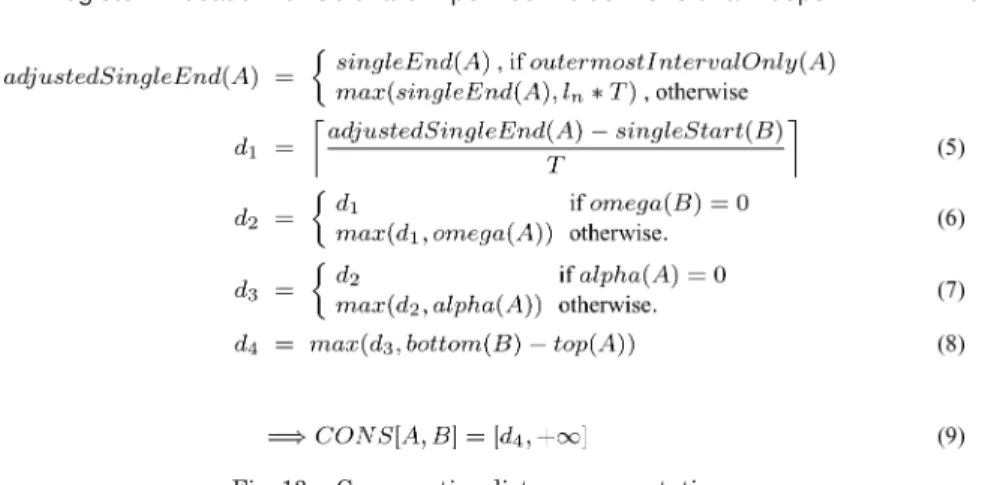
4.3.1 Conservative Distance. First,singleEnd(A) is adjusted. The simplest form of a vector lifetime is composed of the prolog, OLPs, and epilog. In these segments, there should not be any conflict before and after expanding the sim-plest form into the final form. Unfortunately, since ILESes are not included in the simplest form, there is one and only one exception: when a scalar lifetime has an interval (or part of an interval) in the ILES, since the simplest form ab-stracts away the ILES, the scalar lifetime may be shorter than it should be. One may imagine that in the simplest form, an ILES is compressed into a time-line (the end of the OLP before it). In calculating the conservative distance in the simplest form, any scalar lifetime that has an interval within the ILES (i.e.,
Fig. 13. Conservative distance computation.
outermostIntervalOnlyis false) should be treated as if it covers this timeline. We take the first ILES as the reference point in representation for which the time line isln∗T in general.
To compute the conservative distance between two vector lifetimesAandB, we consider the simplest form of the vector lifetimes. The problem is then equiv-alent to that of the single-loop case [Rau et al. 1992] and the following conditions must be verified: the wand ofBmust be to the right of the wand ofA, and the leading/trailing blades of B must be above the leading/trailing blades of A. Formally,
singleStart(B)+(rB−rA)∗T ≥adjustedSingleEnd(A)
rB−rA≥omega(A) if omega(B)>0
rB−rA≥alpha(A) if alpha(A)>0
Solving these inequalities results in formulas (5), (6), and (7) in Figure 13. Next, we further consider the vector lifetimes in their final form . One can think that the final form is the simplest form plus the ILESes. Because inter-leaving is not allowed, ifAandBhave intervals in those segments, a segment of Bshould be above the corresponding segment of A, i.e.,rB−bottom(B) ≥
rA−top(A). This leads us to formula (8).
Example.Figure 14 illustrates the computation ofCONS[TN3,TN1] for the example in Figures 6, 7, and 8. For TN3, it has intervals in the ILESes in the final form as can be seen from Figure 6. Therefore, the singleEnd is adjusted to the end of the first OLP. Then the distance is calculated. D3 ensures that there is no conflict outside the ILESes. Thend4further ensures that there is no conflict inside the ILESes either. In Figure 14(b), we show only the first ILES since any other ILES is simply repetition of it. In this example,d3 =d4 =5, and thusCONS[TN3,TN1]=[5,+∞].
4.3.2 Aggressive Distance. The aggressive distance is the union of the con-servative and interleaving distance. In the following, we introduce how to com-pute the interleaving distance.
Fig. 14. Illustration of conservative distance computation.
First, we consider the ideal form of the vector lifetimes. For each loop level
i, let IAand IBbe the intervals from vector lifetimes Aand Bdefined at this
level, respectively. To interleave them, IB must be put into the hole behind
IA. There is one special case to be considered: if IBis a phantom, the interval
following it in the same scalar lifetime of Bshould be naturally afterIA. That
is,
start(IB)+(rB−rA)∗T ≥ end(IA)
end(IB)+(rB−rA)∗T ≤ nextStart(IA)
next Start(IB)+(rB−rA)∗T ≥ end(IA) ifIBis a phantom,
where start(Iv), end(Iv), and nextStart(Iv) refer to start[i], end[i], and
nextStart[i] of the vector lifetimev, withi ∈ [1,n] being the loop level under discussion.
This leads to the [l,u] range defined by Equations (10) and (11) in Figure 15. The intersection of all the ranges calculated from the (IA,IB) pairs at all loop
levels is the range within which no conflict would occur between A and B. This intersection is defined by Equations (12) and (13) for the lower and upper bounds, respectively.
Fig. 15. Aggressive distance computation.
Then we consider the stretched intervals in the final form. Intuitively, the stretched intervals ofBshould be above the stretched intervals of Aand below the intervals ofAdefined at the inner loop levels. More formally,
rB−bottom(B) ≥ rA−firstStretch(A)
rB−firstStretch(B) ≤ rA−Snif notoutermostIntervalOnly(A).
These translate into formulas (14) and (15).
Finally, similar to formulas (6) and (7), the constraints from the live-in and live-out values are added through formulas (16) and (17).
Example.Figure 16 illustrates the major steps in computing the interleaving distanceINTL[TN3, TN2]for the example in Figures 6, 7, and 8. Here we show only the final form and add the phantom intervals of TN3 to show how the extreme values,+∞and−∞, are used in the formulas naturally without any special concern.
4.4 Bin-Packing on the Cylinder
Once the distance between any two vector lifetimes is computed, the vector lifetimes are inserted one after the other on the surface of a space-time cylinder of a circumference equal to the maximum number of available registers,R. The algorithm is shown in Figure 17.
For any given vector lifetime A,illegal[A] is the set of registers that cannot be allocated to Ato avoid conflict with the already-placed vector lifetimes. Its difference with the full set of available registers, that is, ([0,R−1]−illegal[A]), is the set of candidate registers allocatable toA.
Assume that A is allocated register rA. For any other unallocated vector
Fig. 16. Illustration of aggressive distance computation.
Fig. 18. Calculating the legal/illegal register sets for B, after A is allocated registerrAaround the
space-time cylinder.
of Aor to the left of A. If Bis to be placed to the right of A,rA+DIST[A,B]
is the set of registers that can be allocated toBwithout conflict withA. If Bis placed to the left ofA,rA−DIST[B,A] is this set of registers. The union of the
sets in the two cases is notedlegalSet(B,A). HereDISTis the distance,CONS
orAGGR, andx±setdenotes a new set that is{x±y|∀y ∈set}. The complement ofl e g al Set(B,A) is the set of illegal registers forBdue to conflicts withA.
Figure 18 illustrateslegalSet(B,A) with thin arrows whenDISTisCONS
and bold arrows whenDISTisAGGR. Note that the former is a subset of the latter.
Because the number of physical registers is limited to R, the set of illegal registers wraps around the cylinder and is therefore considered moduloRinto
newIllegal(B,A,R). A legal register before wrapping around the cylinder can become illegal after that if any illegal register after wrapping around overlaps with it as shown by the annotation for parts 1 and 2 in Figure 18.
4.5 Circumference Minimization
So far the solution uses the maximum number of physical registers R as the circumference of the cylinder. The last step tries to compress the cylinder to decrease the actual number of registers required.
First, the circumference is initialized as the distance between the smallest and the biggest registers allocated. Then the allocation is translated such that the smallest register allocated equals 0.
A vector lifetimeAmay conflict with itself after wrapping around the cylinder if the circumference is not withinDIST[A,A], whereDISTis eitherCONSor
Fig. 19. Circumference minimization algorithm. RA andrB refer to the registers allocated to
vector lifetimesAandB, respectively.
illegal register with respect to Aunder the current circumference. If there is no conflict between any pair of vector lifetimes, including a vector lifetime with itself, the search is over. Otherwise, we increment the circumference until a legal solution is found. Note that a circumference ofRis always valid, and thus the search will definitely terminate. The algorithm is shown in Figure 19. 5. PROPERTIES AND TIME COMPLEXITY
LEMMA 1. Lemma 1.Given any two vector lifetimes A and B, if for both A
and B, outmostIntervalOnly is true, then CONS[A,B]=AGGR[A,B].
Intuitively, for a vector lifetime whose outmostIntervalOnlyis true, it has only one interval for each scalar lifetime. Thus putting the vector lifetimeBto the right ofAis equivalent to interleavingBto the right ofA. SoCONS[A,B]=
INTL[A,B]=AGGR[A,B].
PROOF. For any vector lifetime that isoutmostIntervalOnly, according to the definitions in Section 4.2, there are
singleStart = start[1] singleEnd = end[1] nextStart[1] = +∞. And∀i∈[2,n], start[i] = +∞ end[i] = −∞ nextStart[i] = +∞ top = firstStretch bottom = lastStretch+1.
Apply these values to Figures 13 and 15, we have d1 = d5, and d6 = +∞. Then formulas (6)–(9) are equivalent to formulas (14)–(18). Therefore, we have
THEOREM 1. Given two vector lifetimes A and B, if the loop nest is a single
loop (n=1), then CONS[A,B]=AGGR[A,B]=[x,+∞], where x is the lower bound calculated by the classical register allocation for software pipelined single loops [Rau et al. 1992].
In this sense, the approach in this article subsumes the classical approach as a special case.
PROOF. For any vector lifetime in a single loop, outermostIntervalOnly is true. ThereforeCONS[A,B]=AGGR[A,B] according to Lemma 1.
Note that singl eStart is equivalent to start in the traditional case,
singl eEnd is equivalent toend in the traditional case, and (top,bottom) = (+∞,−∞) since there is no ILES. Apply them to the formulas in Figure 13. We obtain exactly the same formulas used in Rau’s method (see Section 2.2).
THEOREM 2. Given any two vector lifetimes A and B, if A has only an interval
defined at the outermost loop level and B only intervals defined at the inner loop levels, then CONS[A,B]=AGGR[A,B].
Intuitively, in this case, the aggressive range just assures thatBis to the right ofA, the same requirement as the conservative range. Thus they become equiv-alent.
PROOF. Let us examine the computation of I N T L[A,B]. For any pair of intervals (IA,IB) from an inner loop leveli ∈ [2,n], their interleaving leads
to a whole range [−∞,+∞]: IA is a phantom, which makes l(IA,IB) in
for-mula (10)−∞since A’send[i] = −∞, andu(IA,IB) in formula (11)+∞since
A’snext Start[i]= +∞.
So the interleaving of the intervals from the outermost loop level will solely determineI N T L[A,B]. Let (IA,IB) be the pair of intervals from the outermost
level. Note thatIBis a phantom andoutmost I nterval Onl y(A) is true. Then
nextStart(IB) = singleStart(B)
end(IA) = singleEnd(A)
nextStart(IA) = +∞.
This makesd5=l(IA,IB)=d1, andd6=u(IA,IB)= +∞.
Similar to the proof of Lemma 1, formulas (6)–(9) are equivalent to formulas (14)–(18). Therefore, we have CONS[A,B] = INTL[A,B] =
AGGR[A,B].
THEOREM 3. Given any two vector lifetimes A and B such that they have
no live-in or live-out values, and have no stretched intervals. Let INTL[A,B]= [x1,x2], and INTL[B,A]=[x3,x4]. If for every level i ∈[1,n], between the pair
of intervals(IA,IB)from A and B at this level, at least one of IA and IB is a
phantom, then[x1,x2]=[−x4,−x3].
PROOF. When the two vector lifetimes have no any live-in and live-out val-ues, or any stretched intervals, from the formulas in Figure 15, we know that
all pairs of (IA,IB) from all loop levels. Similarly,INTL[B,A]=[x3,x4], where
x3=max{l(IB,IA)}, andx4=min{u(IB,IA)}.
IfIAis a phantom, that is,start(IA)= +∞andend(IA)= −∞, then according
to the formulas in Figure 15,
l(IA,IB) = −∞
u(IB,IA) = +∞
and
u(IA,IB) =
next Start(IA)−end(IB)
T
l(IB,IA) =
end(IB)−next Start(IA)
T
= −u(IA,IB).
Therefore,x1= −x4, andx2= −x3.
If IBis a phantom, we have the same conclusion.
Next we analyze the time complexity of our solution. Letl be the total vector lifetimes and o the number of operations. Lifetime normalization and repre-sentation has a time complexity of O(o) per variable, and O(l ∗o) for all the variables. The total time spent in computing distances is O(l2) for all pairs of variables. Sorting can be done inO(l2) time. Bin-packing uses the same strate-gies as those for the single loops [Rau et al. 1992], given the distances. The time complexity for first and end fits are quadratic(O(l2)), and cubic for best fit(O(l3)) [Rau et al. 1992]. Circumference minimization loops at mostRtimes with each time costing O(l2) time. In summary, the overall time complexity is
O(lx+l∗o), wherex =2 for first and end fit strategies, andx =3 for best fit.
6. EXTENSIONS
So far, we assume that a loop nest has operations only between the beginnings of two adjacent loops and the kernel has a single II. In practice, however, it is not uncommon to encounter loop nests that have operations between the ends of two adjacent loops. To achieve better performance, it is also desirable to have multiple IIs. Intuitively, the operations at an inner loop level run more frequently than those at an outer loop level, and therefore should run in a smaller II to shorten the execution time.
In this section, we generalize our solution so that it can be applied to more general loop nests, and then to schedules with multiple IIs.
6.1 Extension to More General Loop Nests
Figure 20(a) shows the more general loop nest. Except for the innermost loop, any other loop Lx(x < n) has two sets of nonbranch operations at its level:
OPSET Ax at the beginning of it, andOPSET Bx at the end of it. The
corre-sponding 1-D schedule (kernel) is shown in Figure 20(b). Note that the last stages of all the loops,l1,l2,. . .,ln, are not necessarily the same. In general,
0= f1≤ f2≤ · · · ≤ fn ≤ln≤ · · · ≤l2≤l1. For a loopLx(x <n), the operations
Fig. 20. The more general model.
either before or after the stages of the inner loopLx+1. The two positions would be referred to asPosAandPosB. For the innermost loop, P os AandP osBare the same. To facilitate understanding, one can simply imagine that operations fromOPSETAxare scheduled toPosA, and those fromOPSETBxare scheduled
toPosB, although this is not necessarily true in general. We assume that at each position for a loop level, a variable either has no definition or has only one definition.
The general form of the final schedule still consists of a prolog, a repetition of an OLP and ILES, and an epilog. It is expressed in the same way as that in Figure 5(c). However, its building block, the kernel, is different.
Example.Figure 21(a) shows an example loop nest which is the same as our previous example in Figure 3(a) except for the operations below the inner loop. Assume the corresponding kernel is that in Figure 21(b). The kernel is such that it will expose the new features of the vector lifetimes and new problems for register allocation, and we ignored the specific resource and dependence con-straints here. The final schedule is in Figure 22, with the ineffective operation instances that are not executed at runtime in darker color.
6.2 New Features of the Vector Lifetimes
With the new loop model, whenl1 > ln, a group enters its ILES before the
previous group fully drains. This leads to an extra feature of a vector lifetime,