EverVIEW: A visualization platform for hydrologic and Earth science
gridded data
Stephanie S. Romañach
a,n, Mark McKelvy
a, Kevin Suir
b, Craig Conzelmann
ba
U.S. Geological Survey, Southeast Ecological Science Center, 3205 College Avenue, Fort Lauderdale, FL 33314, USA bU.S. Geological Survey, National Wetlands Research Center, 700 Cajundome Blvd., Lafayette, LA 70506, USA
a r t i c l e i n f o
Article history:Received 12 April 2014 Received in revised form 4 December 2014 Accepted 11 December 2014 Available online 15 December 2014
Keywords:
Data visualization
Environmental Decision Support Tool Everglades
NASA World Wind NetCDF
Spatial overlay
a b s t r a c t
The EverVIEW Data Viewer is a cross-platform desktop application that combines and builds upon multiple open source libraries to help users to explore spatially-explicit gridded data stored in Network Common Data Form (NetCDF). Datasets are displayed across multiple side-by-side geographic or tabular displays, showing colorized overlays on an Earth globe or grid cell values, respectively. Time-series da-tasets can be animated to see how water surface elevation changes through time or how habitat suit-ability for a particular species might change over time under a given scenario. Initially targeted toward Florida's Everglades restoration planning, EverVIEW has beenflexible enough to address the varied needs of large-scale planning beyond Florida, and is currently being used in biological planning efforts na-tionally and internana-tionally.
Published by Elsevier Ltd. This is an open access article under the CC BY-NC-ND license (http://creativecommons.org/licenses/by-nc-nd/3.0/).
1. Introduction
Restoring an ecosystem is a challenging process that requires a comprehensive understanding of the ecological and physical pro-cesses at work. Making decisions about how to restore an eco-system can be complicated by economic, sociological, and political factors, ranking ecosystem restoration one of the most complex types of environmental decision making (Poch et al., 2004). Eco-system restoration has been described as‘the development and testing of a body of theory for repairing damaged ecosystems' (Palmer et al., 1997). Alternative restoration plans are often pro-posed and can serve as theories for how best to repair damage. Using simulation models of predicted species or habitat responses to restoration, for example, allows these responses to be tested against each restoration theory.
Visualizing model output and other data across the geographic area over which decisions are being made can help quickly iden-tify areas with information gaps, problems with simulation model output, and exploration of hypotheses (Fox and Hendler, 2011). Graphical display of data may be preferential to tabular display for decision making, but information systems research shows this is not always the case (e.g.,Remus, 1984;Dennis and Carte, 1998;
Vessey and Galletta, 1991) and depends on whether spatial in-formation is being conveyed (Vessey, 1991). Given the complexity of restoration decision making, typically across a large spatial ex-tent, development of decision support systems and software tools may allow more informed decision making (Rizzoli and Young, 1997).
The complexity and scale (28,000 km2(Gunderson et al., 1995)) of Florida's Greater Everglades (hereafter‘Everglades’) leads to a vast amount of scientific, economic, and political information to be considered during restoration planning. Everglades restoration aims to return a compartmentalized wetland to a more natural wetland ecosystem with overland waterflow moving southward across the landscape (Gunderson et al., 1995). Ecological and hy-drologic simulation models are being used in restoration planning to examine hydrologic patterns and resulting wildlife responses from proposed restoration plans. Since planning for restoration began two decades ago (U.S. Congress, 2000), scientists have produced vast amounts of biological and hydrologic monitoring data and modeling outputs (e.g.,DeAngelis et al., 1998; Gawlik, 2006;Doren et al., 2009;Jopp et al., 2010;Catano et al., 2014), in a variety of environmental conditions, and over many configurations of potential restoration plans (e.g.,Curnutt et al., 2000;National Research Council, 2012). A challenge began to emerge to make the most informed use of monitoring data and modeling outputs in decision making.
Restoration planners in the Everglades expressed the need to compare alternative restoration plans on their desktops with the Contents lists available atScienceDirect
journal homepage:www.elsevier.com/locate/cageo
Computers & Geosciences
http://dx.doi.org/10.1016/j.cageo.2014.12.004
0098-3004/Published by Elsevier Ltd. This is an open access article under the CC BY-NC-ND license (http://creativecommons.org/licenses/by-nc-nd/3.0/).
nCorresponding author.
E-mail addresses:[email protected](S.S. Romañach),
[email protected](M. McKelvy),[email protected](K. Suir),
ability to explore model inputs and outputs for improved under-standing and informed decision making. Where visualizations were available to examine simulation model output against al-ternative restoration plans, they were often in the form of static maps. Decision makers in the Everglades typically examine four alternative restoration plans during each round of planning. To examine potential impacts of four alternative restoration plans on one species at one point in time means looking at four maps side-by-side. When considering how restoration might affect a species of interest throughout the wet season and the dry season, decision makers need to examine multiple points in time, quickly multi-plying the number of comparisons and maps. Additionally, re-storation efforts consider many biotic and abiotic factors so ana-lysis of output from multiple models complicates the problem even further.
The Everglades ecological modeling community adopted the Network Common Data Form (NetCDF) data format for modeling and visualization. The establishment of a common data format and the Comprehensive Everglades Restoration Plan (CERP) NetCDF Metadata Conventions for the Everglades ecological modeling community formed the foundation for collaborative data sharing among the large number of individuals, state and federal agencies, and other organizations involved in providing information for Everglades restoration planning. At the time, several visualization applications and frameworks existed (e.g. Unidata Integrated Data Viewer (Murray et al., 2003), GRASS GIS (Neteler and Mitasova, 2008), uDig (Ramsey, 2006), and Ncvtk (Pletzer et al., 2005) that fully supported NetCDF, and others (e.g. ArcGIS, ParaView, MA-TLAB) only partially supported NetCDF through supplementary converters. Other drawbacks to these tools included cost and lack of cross-platform support (e.g. ArcGIS), complex user interfaces (e.g. Ncvtk), and technical skill required at setup to support NetCDF (e.g. GRASS GIS). None of the available tools addressed the community needs for simple visualization of ecological and hy-drologic modeling data that could be rapidly developed and iteratively updated in response to active user feedback.
Building on the foundation of a common data format and conventions, the EverVIEW Data Viewer (hereafter‘EverVIEW’) is a free, cross-platform, desktop Java application (Joint Ecosystem Modeling, 2009). EverVIEW was created to bridge the gap between ecological modelers and restoration planners by enabling data from widely varied sources to be readily consumed and made available for use in the decision making process (Romañach et al., 2014).
2. Materials and methods 2.1. Requirements
The initial specifications for EverVIEW were defined and re-fined through in-person meetings with state and federal partners of the Joint Ecosystem Modeling (JEM) community. The key fea-tures that came out of these meetings included the abilities to compare side-by-side map overlays produced from NetCDFfiles, associating specific colors with ranges of values, inspecting and tracking values in particular grid cells, visualizing grid values alongside map overlays, and spatial view synchronization of map overlays. Frequent communication with and feedback from the user community expanded on these initial features to include support for tracking values in groups of grid cells and importing features from common GIS formats (e.g. Environmental Systems Research Institute Shapefile (ESRI, 1998) and Open Geospatial Consortium (OGC) Keyhole Markup Language (KML) (Wilson, 2008)), animation of time-series data, unstructured grids (e.g. triangular or honeycomb meshes), and numerous other features.
2.2. Input data
Since the initial specifications meetings with partners, NetCDF was identified as the primary input format for EverVIEW. NetCDF is an open standard with over two decades of scientific use and was chosen as the modeling output and visualization format by the Everglades ecological modeling community in part because hydrologic datasets in the region were readily available in this form. Although the NetCDF format enables the storage of large amounts of binary, array-based data in a machine-independent way with self-describing metadata (Rew and Davis, 1990), the free-range nature of the metadata specification has contributed to ambiguity associated with user-defined metadata. This ambiguity led to the development of metadata conventions such as the Co-operative Ocean/Atmospheric Research Data Service (Cooperative Ocean/Atmosphere Research Data Service, 1995) and the Climate and Forecast Metadata Conventions (CF) (Gregory, 2003). In 2010, the CERP NetCDF Metadata Conventions (Joint Ecosystem Model-ing, 2010) for orthogonally gridded data, and, later, the CERP Un-structured Grid NetCDF Metadata Conventions (Joint Ecosystem Modeling, 2012), were released with a comprehensive software library to promote code reuse across organizations and lower the barrier to entry for new collaborators in Everglades modeling. EverVIEW was built to support NetCDF datasets adhering to these CERP metadata conventions.
2.3. User interface
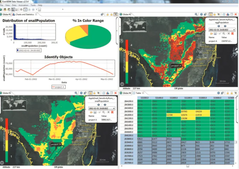
The EverVIEW user interface is organized into a set of globe sections, with each section exposing different views of the loaded data. The views include globe view for colorized overlays on an Earth model,table viewfor inspecting cell values, andchart view for basic summary statistics. The user can add up to eight globe sections, with up to four visible perpage(Fig. 1). Each globe sec-tion shows the data of a single NetCDF variable, any reference layers, and cell value trackers known asidentify objects.
Each globe view supports visualization of a 2D georeferenced NetCDF variable on an Earth model (Figs. 1and2). NetCDF data are displayed in the globe view either as tiled-images layers, which increase in detail as the user's viewpoint gets closer to the surface, orsingle-image layersthat do not increase in detail but offer more performance benefits. Layer colors come from mapping grid cell values to a specificcolor ramp(Fig. 3); a legend is created from the color ramp and shown in the corner of the globe view. The color ramp allows users to create and associate specific colors with ranges of values, or to have a continuous gradient of colors auto-matically generated to correspond with values between the minimum and maximum of the dataset. Only one time step per layer can be visible at one time, so controls are available to step forward and backward through time, select a particular time in-dex, or animate through all time indices. Reference layers are au-tomatically added to the Earth model, such as NASA Blue Marble, i-cubed Landsat, political boundaries, and place names. Status and scale bars show elevation, altitude, and coordinate location under the mouse pointer, as well as scale distances for reference. User interaction with the globe includes zoom, pan, tilt, and roll, via mouse clicking and dragging, scrolling, and key presses. An in-cluded Web Map Service (WMS;de La Beaujardière, 2004) client allows the addition of WMS layers above or below the NetCDF layer.
The table view provides an alternate, more precise view of the loaded NetCDF variable in a familiar, spreadsheet-style tabular format (Figs. 1 and 2). Row and column headers show the co-ordinate values for the spatial extent of the variable, while each table cell shows the value at that particular location and time in-dex. Orthogonal grid data are visualized with one table cell for S.S. Romañach et al. / Computers & Geosciences 76 (2015) 88–95 89
every data cell, while unstructured grid data are sampled at reg-ular intervals, which are adjustable through user preferences. In addition to displaying data cell values, the table cells also have background colors corresponding to the color ramp in use (Figs. 1and 2). The table view automatically displays the same time step that is visible on the globe view.
The chart view displays summary charts of the loaded data, with two charts specific to the current time step and one chart specific to identify objects. Thefirst chart is a histogram showing the distribution of data cell values for the selected time step. The second is a pie chart displaying the total percentage of values for the selected time step that fall within each range defined by the color ramp. Finally, a time-series line chart illustrates how the value of each identify object in the globe section changes over time (Fig. 1).
For identify objects that are composed of a group of points, a polygonal chain, or a polygon, a value can be calculated using the minimum, maximum, or average of all the contained data cells. Identify objects, which are specific to a particular globe section, are visible across all views of a globe section, either by georefer-enced shapes, highlighted table cells, or a chart showing data va-lues over time (Fig. 1).
To facilitate the comparison of datasets, EverVIEW includes synchronization channelsto spatially and temporally link multiple globe sections. A spatial synchronization channel mirrors changes
in altitude and orientation across each synchronized globe section. With this feature enabled, if one globe view is panned or zoomed to view a particular area, all other synchronized globe views in the channel will do the same. Spatial synchronization also copies identify objects from one globe section to others, which allows for detailed comparison among multiple alternative datasets by in-specting the values of identify objects across synchronized views. Similarly, the temporal synchronization channel mirrors the se-lection of a time step to all globe sections in the channel. Used in concert, spatial and temporal synchronization channels allow a user to step through time in multiple datasets and compare tracked locations simultaneously.
The user interface offers twoperspectivesto organize the available globe sections of a page and the views within each section. The defaultmulti-perspectivedisplays up to four globe sections at once in a 22 window configuration (Fig. 1), which stacks the three differ-ent view types within each globe section (globe, table, and chart) such that only one view is visible at a time. The alternative single-perspectiveshows only one globe section per page but allows two views side-by-side for easier exploration of the dataset (Fig. 2).
To simplify the process of loading the same data multiple times, EverVIEW includes the ability to save state configuration files. Thesefiles are saved using Extensible Markup Language (XML;
Bray et al., 1997) and capture the state of either a single globe section or the entire application.
Fig. 1.Multi-perspective showing four sections in view side-by-side. In clockwise order from the top left, we see distribution and time-series charts for simulation model output and area of interest (Globe Section #1, Chart view); color-coded globe overlays for egg population size of a prey species of interest (Globe Section #2; Globe view) and adults of that prey species (Globe Section #3, Globe view), both #2 and #3 showing a hypothetical project area; and color-matched cells and values for adult population (Globe Section #4, Table view).
2.4. Supporting libraries
EverVIEW is built using the Eclipse Rich Client Platform (RCP), which provides reusable user interface controls and mechanisms to bundle, manage, and remotely update the components of a complete software product. Eclipse RCP promotes a modular ap-proach to software design, which improves the maintainability and flexibility of a system while shortening development time (Parnas, 1972; Laplante, 2007). The NASA World Wind software development kit forms the basis of the Earth model used by the globe view and allows multiple georeferenced layer sources (e.g. NetCDF, WMS, NASA Blue Marble) and types (e.g. place-names, political boundaries) to be stacked simultaneously. The GeoTools geospatial library (Turton, 2008), which is built on top of the Java Topology Suite (Davis and Aquino, 2003), underpins much of the projected coordinate system and location transformation func-tionality within EverVIEW and is also a key component of the CERP NetCDF Java library.
3. Results
3.1. Software architecture
EverVIEW takes its design philosophy from the Model-View-Presenter (MVP) software pattern (Potel, 1996), which separates the underlying code structure into three distinct groups: user controls and events (“views”; e.g. globe view, table view, and chart view); data storage and retrieval (“models”); and presentation logic that ties views and models together (“presenters”). A pre-senter attaches to a single model and a single view, mediating between user interaction in the view and state changes in the
model. The advantage of MVP is a moreflexible code structure that promotes maintenance, testing, debugging, and the addition of new features to the software by reducing duplication of similar code. We have added an additional structural grouping to MVP, managers, to aid the synchronization of changes across the models. In contrast to presenters, a manager may attach to two different models (e.g. translating NetCDF variable information into a 2D georeferenced globe layer), or it may attach to multiple models of the same type (e.g. synchronizing identify objects across different globe sections).
The largest and most important model within EverVIEW, the data model, stores information for a particular globe section and is composed of multiple smaller models. For example, one such subcomponent of the data model is thedata access model, which makes extensive use of the CERP NetCDF library, keeps track of the loaded NetCDF file (e.g. file location, variable, coordinates, and time index), and generalizes the differences between the ortho-gonal and unstructured grid files so that common subset opera-tions can be performed spatially and temporally when retrieving values; other subcomponents in the data model include a color ramp model and models for loaded identify objects. By grouping logically similar components into their own models, we promote code reuse and testability. For example, EverVIEW uses custom presenters that know how to interact with each view type, thereby reusing and sharing the data model across the three views of a globe section.
Other models exist, such as the World Wind-basedglobe model, that cannot be reused by multiple presenters. Associated with the globe view, the globe model stores information about the NetCDF time-series layers, World Wind-specific surface shapes for identify objects and their annotations, and reference layers such as place names that come from WMS. These concepts do not relate to the Fig. 2.Single-perspective showing alternate globe and table views of the same dataset side-by-side.
table or chart views, and are best kept separate from state in-formation common to all views. However, we still benefit from reuse since globe models are shared by synchronization managers that operate across globe sections.
3.2. Software execution
During application initialization, the initial globe section and globe view are tied via separate presenters to a new data model instance and a new globe model instance, which are maintained while the globe section is open. At this point, the data model contains no references to identify objects, a color ramp, or a NetCDFfile, and is not synchronized spatially or temporally. The globe model has only the default reference layers (NASA Blue Marble, political boundaries, and place-names) enabled.
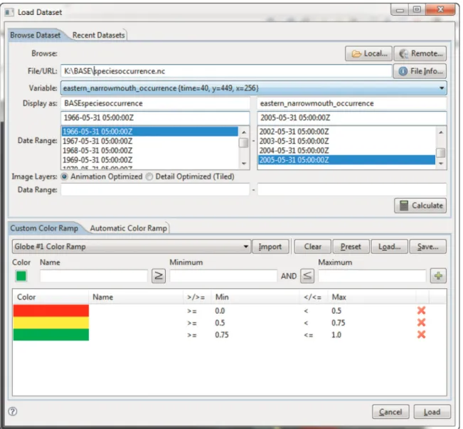
Along with the initialization for the globe section, adata loader presenter is created and attached to the data model and a new instance of thedataset loader dialogas its view (in the MVP sense). The dataset loader dialog allows browsing to a local NetCDFfile (Fig. 3) or accessing a remote dataset using the Open source Pro-ject for a Network Data Access Protocol (OPeNDAP;Cornillon et al., 2003). When the user requests to load a new dataset, the data loader presenter resets the view and makes it visible. The pre-senter handles all events from the view, including showing a list of
available data variables and a range of dates available for the de-fault selected variable. The presenter handles the determination of available data variables; it scans the NetCDFfile for variables that follow the CERP NetCDF Metadata Conventions and have spatial dimensions (such as x and y for orthogonal grids), a valid co-ordinate reference system (CRS) (via the‘grid_mapping’attribute), and an optional time dimension. The user selects a data variable and date range on the view, then configures the color ramp. After the user has customized the dataset parameters and color ramp, the‘load’click event causes the presenter to reset the data model's state, initialize a new data access model, and set a new color ramp. Following these actions by the data loader presenter, other pre-senters and managers attached to the data model are notified that new data have been loaded.
It is the responsibility of thedata loaded managerto propagate the appropriate changes between the data model and the globe model. This manager establishes a unique key for the selectedfile, variable, date range, and color ramp, which is used as a cache directory name for the data layer images that will be generated. The images are cached on thefile system so they can be reused on subsequent loads. After determining whether the new data layers will be single-image layers or tiled-images layers, the data loaded manager creates layers capable of displaying orthogonal or un-structured grid data–making use of the generalized data access Fig. 3.Dataset loader dialog allows configuring the inputfile, data variable, and time range selection, as well as customization of the color ramp used to influence the display of the legend, globe overlays, and table cells.
model – without actually being aware of which is used. Tiled-images layers are automatically used if the data variable has a large number of (spatial) cells to increase performance and reduce memory consumption. Finally, the manager propagates the layer group to the globe model and theimage caching manageris noti-fied that new data are ready, which works independently in the background to generate the single-images or initial tiled-images for each time step.
Thedata presenter, which is also connected to the data model and an abstracted view (reused by the globe, table, and chart views), is responsible for the interaction that takes place when identify objects are added. The abstracted view exposes the con-trols that enable identify mode, if it is supported, and commu-nicates click and location information used to create identify ob-jects to the data presenter via event listeners. The data presenter is unaware of the view type from which it receives events; its only concern at this point is to add the identify object to its model. The data presenter handles the view-to-model interaction for new identify objects, while other presenters are tasked with model-to-view display of identify objects due to differences in the model-to-view type. Before adding an identify object, the data presenter determines if the model has valid data, if new identify objects are allowed, and which types can be added. The presenter communicates to the user through the view to prompt for the identify object type and begin the creation process. The view uses minimal logic to convert user interaction events into world coordinates beforefiring loca-tion event data to its presenter. The presenter converts world co-ordinates to the dataset-native CRS before adding the identify object to its model. The presenters for model-to-view display of identify objects receive an event from the model after the identify object is added and take the necessary steps to display it on its attached view. For example, thetable presenterwill scroll the table view to the associated cells and highlight them, and the chart presenterwill update the time-series chart of identify objects if the data are temporal (Fig. 1). Because of their unique nature, the World Wind-based globe model and view are updated by using theidentify synchronization manager, connected to the data model and globe model, instead of with a presenter. The data presenter has only one small role in the model-to-view display of identify objects; it updates its attached view with the name and value of the newly added identify object.
For identify object synchronization that occurs between globe sections on the same channel, the complete list of identify objects on the channel needs to be determined. The list is aggregated from every globe section on the channel, and because identify object coordinates are defined in a dataset-native CRS for each globe section, the coordinates are transformed to a common reference frame of World Geodetic System 1984 (WGS84) latitude and longitude. Duplicates are eliminated by testing that each identify object will be accepted by each data model, and then the identify synchronization manager sets thefiltered list to each data model on the channel. From there, within-globe section synchronization occurs to propagate changes from the data model to the globe model and views of each globe section.
The synchronization of information within and between globe sections can become complicated. For simplicity, different types of interaction are handled by different managers.
Within-globe section interactions occur between the data model and globe model and can include:
data loading, date index changes, identify objects, location focusing (for identify objects), and loading or saving of globe section state information (e.g., open views and identify objects).Between-globe section synchronization is needed for the data
and globe models of all globe sections and covers:
maintaining a list of recently loaded datasets and parameters, animation of time steps, selected spatial channel, World Wind viewpoints, and iden-tify objects, selected temporal channel and selected dates, identify objects, and loading or saving of application-level state information (e.g., globe section-level state information plus multi- or single-perspective).There is at least one manager dedicated to carrying out each item in the lists above, and in the case of spatial channels, multiple managers tailored to unique tasks. When information is loaded from globe- or application-level state configurationfiles, a man-ager handles the state initialization of the data model, and other managers and presenters handle the rest–including open views and perspective type, restoring open globe sections, spatial and temporal synchronization, etc.
4. Discussion
EverVIEW has met a critical need to visualize ecological and hydrologic modeling outputs in the Greater Everglades (Romañach et al., 2014). Decision makers have benefitted from the ability to spatially synchronize and compare wet and dry seasons side-by-side, animate time-series to see patterns, and track regions of in-terest such as water management areas imported from shapefiles. The Everglades modeling community has provided ongoing feed-back on the iterative development of EverVIEW and thus bene-fitted from the addition of those decision-support features most needed by users. The choice of using open standards and libraries, as well as a modular software architecture, has allowed the de-velopment of EverVIEW to be flexible enough to respond to changing needs.
The decision to create and use the CERP NetCDF conventions within EverVIEW has been very beneficial for collaboration, data sharing, and development among the Everglades modeling com-munity. The CERP NetCDF library has allowed an entire suite of modeling and decision-support tools to operate around a con-sistent set of conventions, including not only EverVIEW, but also models developed by various Everglades restoration partner agencies (e.g.,Pearlstine et al., 2011;Romañach et al., 2011a; Ro-mañach et al., 2011b; Lo Galbo et al., 2012;Shinde et al., 2013). This has resulted in less development overhead for edge cases (e.g. the lack of coordinate variables, lack of standard attributes, or uncommon grid storage types) by reducing ambiguity in the types of input that applications are expected to handle, and thus, these applications are more reliable and use fewer lines of code, while the data they produce are more consistent.
Testing new versions of EverVIEW occurs principally in Win-dows, the operating system most common amongst EverVIEW users, with spot testing on Mac OS X and, to a lesser degree, Ubuntu Linux. A small group of users and developers follow a scripted guide through new features being introduced via user stories, regression tests targeting recently changed code, and sampling tests targeted at other, unrelated and unchanged areas of the application. The scripted guide also includes testing with currently or historically problematic datasets that push EverVIEW to its limits in handling spatial detail and/or temporal breadth. Testing results and issues are recorded both in the scripted guide and in a bug tracking system. This process typically occurs in multiple phases, resulting in the internal release of 1-2 alpha versions before each major release. Once internal testing is com-plete, a production version is released to the public in a stable but notfinal state, commonly known as permanent beta. Production S.S. Romañach et al. / Computers & Geosciences 76 (2015) 88–95 93
releases of EverVIEW include detailed help documentation and capabilities for users to contact developers with feature requests or report bugs as they happen. Feature requests are regularly logged, assessed, and incorporated into the development cycle, while bug reports typically lead to a live update of the current production software.
Though originally developed for scientists in the Everglades community, EverVIEW use has grown beyond Everglades-specific restoration projects, such as the Central Everglades Planning Pro-ject, and assessing the impacts of restoration plans. For example, EverVIEW was used for the Conservation Effects Assessment Pro-ject (CEAP), a national initiative from the United States Depart-ment of Agriculture's, National Resources Conservation Service. As part of the CEAP modeling of the Mississippi River Alluvial Valley, EverVIEW and other tools were used by decision makers to vi-sualize datasets like total carbon for vegetation samples along the valley. During the Mechanical and Technical Review of modeling inputs and outputs for Louisiana's 2012 Master Plan (Coastal Pro-tection and Restoration Authority of Louisiana, 2012), EverVIEW was used to review large volumes of eco-hydrology, wetland morphology, and ecosystem services modeling outputs.
Ongoing development of EverVIEW will continue to be funded by and address the needs of partners within and beyond the Everglades ecological modeling community. An extension-based application programming interface has been developed so that custom tools and environments can be developed that leverage EverVIEW as a platform. Examples of such tools that have already been developed include a basic screenshot capture tool, a shapefile to NetCDF converter, a tool used to explore climate envelope models for threatened and endangered species, and an environ-ment for visualizing future scenarios of potential climate and ur-banization changes in Florida.
Acknowledgments
Funding for software development was provided by the U.S. Geological Survey's Greater Everglades Priority Ecosystem Science. Use of trade, product, orfirm names does not imply endorsement by the US Government. We are grateful for comments by Leonard Pearlstine and two anonymous reviewers that helped improve this manuscript.
Appendix A. Supplementary information
Supplementary data associated with this article can be found in the online version atdoi:10.1016/j.cageo.2014.12.004.
References
Bray, T., Paoli, J., Sperberg-McQueen, C.M., Maler, E., Yergeau, F., 1997. Extensible
markup language (XML). World Wide Web J. 2, 27–66.
Catano, C.P., Romañach, S.S., Beerens, J.M., Pearlstine, L., Brandt, L., Hart, K.M., Mazzotti, F.J., Trexler, J.C., 2014. Using scenario planning to evaluate the impacts of climate change on wildlife populations and communities in the Florida Everglades. Environ. Manag., http://dx.doi.org/10.1007/s00267-014-0397-5. Coastal Protection and Restoration Authority of Louisiana, 2012. Louisiana's
Com-prehensive Master Plan for a Sustainable Coast. Coastal Protection and Re-storation Authority of Louisiana, Baton Rouge, LA.
Congress U. S., 2000. Water Resources Development Act 2000. Public law number 106-541.
Cooperative Ocean/Atmosphere Research Data Service (COARDS), 1995. Cooperative Ocean/Atmosphere Research Data Service Conventions. ftp://ftp.unidata.ucar. edu/pub/netcdf/Conventions/COARDS/README. (Retrieved 07.11.13).
Cornillon, P., Gallagher, J., Sgouros, T., 2003. OPeNDAP: accessing data in a dis-tributed, heterogeneous environment. Data Sci. J. 2, 164–174.
Curnutt, J.L., Comiskey, J., Nott, M.P., Gross, L.J., 2000. Landscape-based spatially
explicit species index models for Everglades restoration. Ecol. Appl. 10,
1849–1860.
Davis, M., Aquino, J., 2003. Jts topology suite technical specifications, ,. Vivid So-lutions Victoria, British Columbia.
de La Beaujardière, J., 2004. OGC Web Map Service Interface, version 1.3. 0. Open Geospatial Consortium.
DeAngelis, D.L., Gross, L.J., Huston, M.A., Wolff, W.F., Fleming, D.M., Comiskey, E.J., Sylvester, S., 1998. Landscape modeling for Everglades ecosystem restoration. Ecosystems 1, 64–75.
Dennis, A., Carte, T., 1998. Using geographical information systems for decision making: extending cognitivefit theory to map-based presentations. Inf. Syst. Res. 9, 194–203.
Doren, R.F., Trexler, J., Gottleib, A., Harwell, M., 2009. Ecological indicators for system-wide assessment of the greater everglades ecosystem restoration pro-gram. Ecol. Indic. 9, S2–S16.
ESRI, 1998. Shapefile Technical Description, Environmental Systems Research In-stitute, Inc.
Fox, P., Hendler, J., 2011. Changing the equation on scientific data visualization. Science 331, 705–708.
Gawlik, D.E., 2006. The role of wildlife science in wetland ecosystem restoration: lessons from the Everglades. Ecol. Eng. 26, 70–83.
Gregory, J., 2003. The CF metadata standard. CLIVAR Exch. 8 (4).
Gunderson, L.H., Light, S.S., Holling, C.S., 1995. Lessons from the Everglades. BioScience, S66–S73.
Joint Ecosystem Modeling, EverVIEW Data Viewer, 2009.〈http://www.jem.gov/ Modeling〉. (Retrieved on 06.11.13).
Joint Ecosystem Modeling, Orthogonal NetCDF Standard, 2010.〈http://www.jem. gov/〉.Standards last accessed (Retrieved 06.11.13).
Joint Ecosystem Modeling, Unstructured Grid NetCDF Standard, 2012.〈http://www. jem.gov/Standards〉.(Retrieved 06.11.13).
Jopp, F., DeAngelis, D.L., Trexler, J.C., 2010. Modeling seasonal dynamics of smallfish cohorts influctuating freshwater marsh landscapes. Landsc. Ecol. 25,
1041–1054.
Laplante, F., 2007. What Every Engineer Should Know About Software Engineering. CRC Press, Boca Raton, Florida.
Lo Galbo, A., Pearlstine, L., Lynch, J., Fennema, R., Supernaw, M., 2012. Wood Stork Foraging Probability Index (STORKI v. 1.0) Ecological and Design Documenta-tion. South Florida Natural Resources Center, Everglades National Park, National Park Service, Homestead, Florida, 25 pp.〈http://www.cloudacus.com/sim glades/docs/WoodStorkEcologicaldoc_20120601.pdf〉.(Retrieved 06.11.13). Murray, D., McWhirter, J., Wier, S., Emmerson, S., 2003. 13.2 The integrated data
viewer: a web-enabled application for scientific analysis and visualization. In: Proceedings of the 19th International Conference on Interactive Information and Processing Systems for Meteorology, Oceanography, and Hydrology.
National Research Council, 2012. Progress toward restoring the everglades: the
fourth biennial review, Committee on Independent Scientific Review of
Ever-glades Restoration Progress (CISRERP).. National Academies Press. Washington,
DC: The National Academies Press, pp. 149–176 (Chapter 5).
Neteler, M., Mitasova, H., 2008. Open Source GIS: A GRASS GIS Approach, 3rd edn. Springer, New York, NY, p. 406.
Palmer, M.A., Ambrose, R.F., Poff, N.L., 1997. Ecological theory and community re-storation ecology. Restor. Ecol. 5 (4), 291–300.
Parnas, D.L., 1972. On the criteria to be used in decomposing systems into modules.
Commun. ACM 15, 1053–1058.
Pearlstine, L., Friedman, S., Supernaw, M., 2011. Everglades Landscape Vegetation Succession Model (ELVeS) Ecological and Design Document: Freshwater Marsh & Prairie Component version 1.1. South Florida Natural Resources Center, Everglades National Park, National Park Service, Homestead, Florida, 128 pp.
〈http://www.cloudacus.com/simglades/docs/ELVES%20freshmarsh%
20Ecological%20Doc_v1-1_30July2011.pdf〉. (Retrieved 12.11.13).
Pletzer, A., Ziemlinski, R., Cohen, J., 2005. Ncvtk: A program for visualizing plane-tary data, Computational Science–ICCS 2005. Springer, Berlin Heidelberg, pp.
838–841.
Poch, M., Comas, J., Rodriguez-Roda, I., Sanchez-Marre, M., Cortés, U., 2004. De-signing and building real environmental decision support systems. Environ. Model. Softw. 19 (9), 857–873.
Potel, M., 1996. MVP: Model-View-Presenter the Taligent Programming Model for Cþ þand Java, Taligent Inc.
Ramsey, P., 2006. uDig desktop application framework. In: Proceedings of the Presentation at the FOSS4G Conference, Lausanne, Switzerland.
Remus, W., 1984. An empirical investigation of the impact of graphical and tabular
data presentations on decision making. Manag. Sci. 30, 533–542.
Rew, R.K., Davis, G.P., 1990. NetCDF: an interface for scientific data access. IEEE Comput. Graph. Appl. 10, 76–82.
Rizzoli, A.E., Young, W.Y., 1997. Delivering environmental decision support systems: software tools and techniques. Environ. Model. Softw. 12 (2–3), 237–249. Romañach, S.S., Conzelmann, C., Daugherty, A., Lorenz, J.L., Hunnicutt, C., Mazzotti,
F.J., 2011a. Joint Ecosystem Modeling (JEM) Ecological Model Documentation Volume: Roseate Spoonbill (Platalea ajaja) Landscape Habitat Suitability Index v1.0.0: U.S. Geological Survey Open-File Report 2011–1273, 23 pp.〈http://pubs. usgs.gov/of/2011/1273〉. (Retrieved 06.11.13).
Romañach, S.S., Conzelmann, C., Daugherty, A., Lorenz, J.T., Hunnicutt, C., Mazzotti, F.J., 2011b. Joint Ecosystem Modeling (JEM) Ecological Model Documentation Volume 1: Estuarine Prey Fish Biomass Availability v1.0.0: U.S Geological Sur-vey Open-File Report 2011–1272, 20 pp.〈http://pubs.usgs.gov/of/2011/1272/〉. (Retrieved 06.11.13).
Romañach, S.S., McKelvy, M., Conzelmann, C., Suir, K., 2014. A visualization tool to support decision making in environmental and biological planning. Environ. Model. Softw. 62, 221–229.
Shinde, D., Pearlstine, L., Brandt, L.A., Mazzotti, F.J., Parry, M., Jeffery, B., LoGalbo, A., 2013. Alligator Production Suitability Index Model (GATOR-PSIM v. 1.0). Eco-logical and Design Documentation, 38 pp.〈http://www.cloudacus.com/sim glades/docs/AlligatorEcologicaldoc_releaseV1.0_review_apr2013.pdf〉. (Re-trieved 06.11.13).
Turton, I., 2008. Geo tools. In Open Source Approaches in Spatial Data Handling.
Springer, Berlin Heidelberg, pp. 153–169.
Vessey, I., 1991. Cognitivefit: a theory-based analysis of the graphs versus tables literature. Decis. Sci. 22, 219–240.
Vessey, I., Galletta, D., 1991. Cognitivefit: an empirical study of information ac-quisition. Inf. Syst. Res. 2, 63–84.
Wilson, T., 2008. OGC Keyhole Markup Language 2.2.0. Open GIS Consortium.