An Investigation of Missing Data Methods for Classiffcation Trees

(1)

An Investigation of Missing Data Methods for

Classification Trees

Yufeng Ding

∗

Jeffrey S. Simonoff

∗

December 3, 2006

Abstract

There are many different missing data methods used by classification tree algorithms, but few studies have been done comparing their appropri-ateness and performance. This paper provides both analytic and Monte Carlo evidence regarding the effectiveness of six popular missing data methods for classification trees. We show that in the context of classifi-cation trees, the relationship between the missingness and the dependent variable, rather than the standard missingness classification approach of Little and Rubin (2002) (missing completely at random (MCAR), miss-ing at random (MAR) and not missmiss-ing at random (NMAR)), is the most helpful criterion to distinguish different missing data methods. We make recommendations as to the best method to use in various situations. The paper concludes with discussion of a real data set related to predicting bankruptcy of a firm.

Keywords: C4.5, CART, Classification tree,rpart, Separate class.

1 CLASSIFICATION TREES AND THE

PROBLEM OF MISSING DATA

Classification trees are a supervised learning method appropriate for data where the dependent variable is categorical. The predictors can be either cat-egorical or continuous. The simple methodology behind classification trees is to recursively split data based upon the predictors that best distinguish the dependent variable classes. There are, of course, many subtleties, such as the choice of criterion function used to pick the best split variable, stopping rules, pruning rules, and so on. Details about classification trees can be found in vari-ous references, e.g. Breiman, Friedman, Olshen, and Stone (1998) and Quinlan (1993).

Like most statistics or machine learning methods, “base form” classification trees are designed assuming that data are complete. However, missing data is a ∗_{New York University, Stern School of Business, 44 West 4th Street, New York, N.Y. 10012}

(2)

very common problem, and for this reason classification trees have to, and do, have ways of dealing with missing data in the predictors (in supervised learning, an observation with missing response value has no information about the un-derlying relationship, and must be omitted). Although there are many different ways of dealing with missing data in classification trees, there are few studies in the literature about the appropriateness and performance of these missing data methods. In this paper, we compare many popular missing data methods in a systematic way in order to provide understanding of their appropriateness and performance. Assuming there are missing values in the training set, we show that the relative performance of different missing data methods depends on two factors, whether or not the testing set contains missing values and whether or not the missingness depends on the target variable. As will be detailed later, the first factor reveals that the missingness is part of the data generating process and can be helpful when it exists in both the training phase and the testing phase. So far as we are aware, this fact has been largely ignored. The second factor argues against the blind use of the MCAR, MAR and NMAR of Little and Rubin (2002), which has been shown to be helpful with likelihood-based or Bayesian analysis.

Section 2 gives a brief introduction to the previous research on this topic. This is followed by discussion of the design of this study in Section 3 and findings in Section 4. Application to a bankruptcy prediction problem is given in Section 5. We conclude with discussion of these results and future work in Section 6.

2 PREVIOUS RESEARCH

There are few studies of missing data and classification trees in the literature. Liu, White, Thompson, and Bramer (1997) gave a general description of the problem, but did not discuss solutions. Saar-Tsechansky and Provost (2006) discussed various missing data methods in classifications trees and proposed a cost-sensitive approach to the missing data problem for the scenario when missing data occur only at the testing phase, which is different from the problem studied here (where missing values occur in the training phase).

Kim and Yates (2003) conducted a simulation study of seven popular miss-ing value methods but did not find any dominant method. Feelders (1999) did a comparative experiment on the performance of surrogate split and imputa-tion and found the imputaimputa-tion methods to work better. (These methods are described more fully in the next section.) Batista and Monard (2003) com-pared four different missing data methods, and found that 10 nearest neighbor imputation outperformed other methods in most cases. In the context of cost sensitive classification trees, Zhang, Qin, Ling, and Sheng (2005) studied four different missing data methods based on their performances on five data sets with artificially generated random missing values. They concluded that the in-ternal node method (the decision rules for the observations with the next split

(3)

variable missing will be made at the (internal) node) is better than the other three methods examined.

Weaknesses of all of these studies are that they were all based on only a few data sets, and missingness was independent of all of the data (missing completely at random, using the nomenclature of Little and Rubin, 2002). The study described in the next section addresses these issues by allowing for different data sets and different missingness mechanisms. We provide both analytical results for simple situations and Monte Carlo comparisons for more complex ones.

3 THE DESIGN OF THE STUDY

There are essentially two stages of applying classification trees, the learning phase where the historical data (training set) are used to construct the tree, and the testing phase where the tree is applied to testing data. This study deals with the scenario where missing data occur in the training set, while the testing set may be either complete or incomplete. Our results show that the relative performances of different missing data methods are different depending on whether or not the testing set contains missing values.

Accuracy, calculated as the percentage of correctly classified observations, is usually used to measure the performance of classification trees. Since it can be affected by both the data structure (some data are intrinsically easier to classify than others) and by the missing data, this is not necessarily a good measure for the impact of missing data. In this study, we define a measure calledrelative accuracy (RelAcc), calculated as

RelAcc= Accuracy with missing data Accuracy with complete data.

This can be thought of as a standardized accuracy, as RelAcc measures the accuracy achievable with missing values relative to that with complete data.

The recursive nature of classification trees makes them almost impossible to analyze analytically in the general case beyond 2×2 tables (where there is only one binary predictor and a binary target variable). On the other hand, trees built on 2×2 tables can be considered as degenerate classification trees, as a classification tree is built (recursively) as a hierarchy of these degenerate trees. Therefore, analyzing 2×2 tables can have important implications for more general cases. In this study, we start with analysis of 2×2 tables. We then build on this using simulations, where the factors that might have impacts on performance are incrementally added, in order to see the effect of each factor. The factors include variation in both the data generating process (DGP) and the missing data generating process (MGP), the number and type of predictors in the data, and the number of predictors that contain missing values.

This study examines six different missing data methods: probabilistic split, complete case method, grand mode/mean imputation, separate class, surrogate

(4)

split, and complete variable. Probabilistic split is the default method of C4.5 (Quinlan, 1993). In the training phase, observations with values observed on the split variable are split first. The ones with missing values are then put into each of the child nodes with a weight given as the proportion of non-missing instances in the child. In the testing phase, an observation with a missing value on a split variable will be associated with all of the children using probabilities, which are the weights recorded in the training phase. The complete case method deletes all observations that contain missing values in any of the predictors in the training phase. If the testing set also contains missing values, complete case is not applicable and thus some other method has to be used. In the simulations, we use C4.5 to realize the complete case method. In the training phase, we manually delete all of the observations with missing values and then run C4.5 on the pre-processed complete data. In the testing phase, the default missing data method, probabilistic split, is used. Grand mode imputation imputes the missing value with the grand mode of that variable if it is categorical. Grand mean is used if the variable is continuous. The separate class method treats the missing values as a new class (category) of the predictor. Surrogate split is the default method of CART (realized using rpart in this study; Breiman et al., 1998 and Therneau and Atkinson, 1997). It finds and uses a surrogate variable (or several surrogates in order) within a node if the variable for the next split contains missing values. In the testing phase, if a split variable contains missing values, the surrogate variables in the training phase are used instead. The complete variable method simply deletes all variables that contain missing values.

4 THE EFFECTIVENESS OF MISSING

DATA METHODS

This study covers the situations where missing data occur in the training phase. There are, however, still two different scenarios: when missing data do not occur in the testing phase and when missing data occur in the testing phase. If the testing set is complete, then the purpose of the classification tree in the training phase is to uncover the true DGP. In this case, the existence of missing values in the training phase is a only a problem, since they obscure the underlying DGP. However, if the testing set also contains missing values, then the missingness is part of the data and the MGP becomes an essential part of the DGP. This, of course, requires the assumption that the MGP (as well as the DGP) is the same in both the training phase and the testing phase. These two different scenarios can be exemplified as in Example 1.

Example 1. Consider a public historical bankruptcy data set, which contains missing values due to various reasons, such as (for example) certain companies failing to submit their financial statements. There are two users of the data, A and B, who are both interested in predicting if company C is going to bankrupt.

(5)

However, A is the CEO of company C, and thus has all the financial information about his own company, while B is an outside analyst who has to rely on the public information about company C that may have some information missing. In this example, missing values in the historical data are only a problem to A since they hinder his ability to learn about the underlying relationship (DGP) between the financial figures and bankruptcy. However, missingness may not necessarily be a problem to B if, for example, historically, companies that fail to report some key items tend to go bankrupt, since if company C fails to report those key figures that is a strong indicator of potential bankruptcy.

As will be seen, under these two different scenarios, the relative performances of the missing data methods are different.

In this section, we first present analytical results, assuming there is no de-viation from the underling true DGP/MGP (that is, the data reflect exactly the underlying DGP/MGP) and also assuming there are enough data so that the impact of stopping rules and pruning can be ignored. Proofs to the theo-rems can be found in the Appendix. Some of these results are for 2×2 tables only, but as will be seen, they have general implications when added factors are included. The usefulness of these results is that they allow examination of “consistency”-type results, in the sense that they reflect expected performance when the sample size is very large.

4.1 Analytical results

Theorem 1. If the MGP is conditionally independent of Y givenX, then the tree built on the data containing missing values gives the same set of rules as the tree built on the complete data set.

Theorem 2. If the partition of the data defined by the tree built on the incom-plete data is not changed from the one defined by the tree built on the comincom-plete data, the loss in accuracy when the testing set is complete is bounded above by PM, where PM is the missing rate, defined as the percentage of observations

that contain missing values.

Theorem 3. If the partition of the data defined by the tree built on the incom-plete data is not changed from the one defined by the tree built on the comincom-plete data, the relative accuracy when the testing set is complete is bounded below by

RelAccmin =1−PM

1 +PM,

wherePM is the missing rate.

Theorem 4. In a 2×2 data table, if the MGP is independent of eitherY orX, given the other variable, then the following results hold for probabilistic split.

1. IfX is not informative in terms of classification, i.e. the majority classes of Y for different X values are the same, then probabilistic split will give the same rule as the one that would be obtained from complete data;

(6)

2. If probabilistic split shows thatX is informative in terms of classification, i.e. the majority classes ofY for different X values are different, then it finds the same rule as the one that would be obtained from complete data; 3. The absolute accuracy when the testing set is complete is bounded below by 0.5. Since the complete data accuracy is at most 1, the relative accuracy is also bounded below by 0.5.

Theorem 5. If the MGP is independent of Y, given X, then the same re-sults hold for mode imputation as for probabilistic split under the conditions of Theorem 4.

Theorems 1, 2 and 3 (for the complete case method) are true for general data sets. Theorems 4 and 5 are for 2×2 tables only but they imply that probabilistic split and mode imputation have advantages over the complete case method, which can have very poor performance (as shown later in Figure 1).

With 2×2 tables, the complete variable method will always have a higher than 0.5 accuracy since by ignoring the only predictor, we will always classify all of the data to the overall majority class and achieve at least 0.5 accuracy. This is not readily generalizable, however, given that deleting the whole variable is an extreme measure. Simulations will show the performance of complete variable method in more general cases.

Surrogate split is not applicable with 2×2 tables because there are no other predictors. For 2×2 table problems with a complete testing set, separate class is essentially the same as the complete case method, because as long as the data are split according to the predictor (and it is very likely that this will be so), the separate class method builds separate rules for the observations with missing values; when the testing set is complete, the rules that are used in the testing phase are exactly the ones built on the complete observations. This, however, is less likely to be true when there are more predictors and/or continuous predictors, because the extra class for the missingness will affect the information gain and thus result in a different tree if the separate class method is used. This difference, as will be seen, tends to have a favorable impact on the accuracy performance.

When the testing set also contains missing values, the following theorem holds.

Theorem 6. In 2×2 data tables, if missing values occur in both the training set and the testing set, then the separate class method has the best performance. Theorem 6 makes a fairly strong statement in the simple situation, and it will be seen to be strongly indicative of the results in more general cases. Its proof also can be found in the Appendix.

The analytical results shows that the complete case method has the best (perfect) expected performance when the test set is complete and the miss-ingness does not depend on the target variable. The results also imply that

(7)

probabilistic split and mode imputation may have a better performance when the conditions of Theorems 4 and 5 are satisfied. When the test set is incom-plete, separate class is expected to have the best performance. To verify these results and extend the understanding of the performance of different missing data methods to general cases, we carry out two types of Monte Carlo simula-tions. In the next section, we do a Monte Carlo simulation of the DGP/MGPs of 2×2 tables. In this simple case, the expected tree performance can be worked out given the DGP/MGP and the simulations can be used to verify the de-rived analytical results. In the following section, we carry out large scale Monte Carlo simulations of data sets with more predictors and continuous predictors. In these simulations, data sets are generated according to the randomly gener-ated DGP/MGPs, so random deviations from the true DGP/MGP are present, allowing examination of the effects of this random variation.

4.2 Monte Carlo Simulations for 2

×

2 tables

4.2.1 A brief description of the simulations

A 2×2 table with missing values has only eight cells as shown in Table 1, where M = 0 ifX is observed andM = 1 ifX is missing.

M X Y P 0 0 0 P(M = 0, X= 0, Y = 0) 0 0 1 P(M = 0, X= 0, Y = 1) 0 1 0 P(M = 0, X= 1, Y = 0) 0 1 1 P(M = 0, X= 1, Y = 1) 1 0 0 P(M = 1, X= 0, Y = 0) 1 0 1 P(M = 1, X= 0, Y = 1) 1 1 0 P(M = 1, X= 1, Y = 0) 1 1 1 P(M = 1, X= 1, Y = 1)

Table 1: The 8 cells of a 2×2 table with missing values

There is one constraint, that the sum of the probabilities has to be one. Therefore, this table is determined by seven parameters, but which seven to use is arbitrary. To illustrate the true DGP and MGP, the following seven parameters are used:

1. P(X = 0) 2. P(Y = 0|X = 0) 3. P(Y = 0|X = 1) 4. P(M = 0|X = 0, Y = 0) 5. P(M = 0|X = 0, Y = 1)

(8)

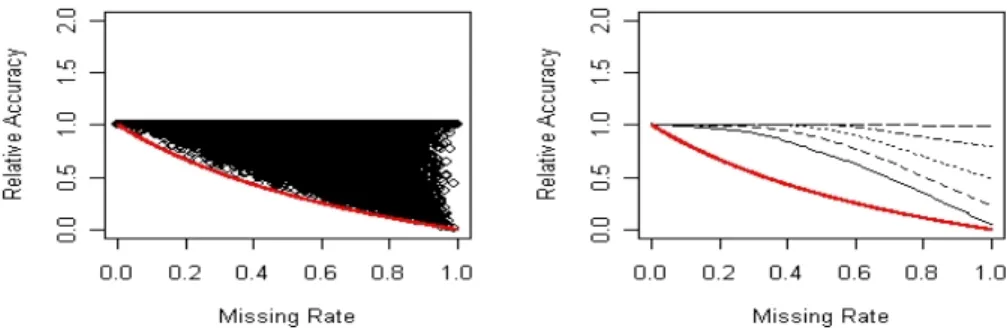
Figure 1: Scatter plot and the corresponding quantile plot of the complete testing setRelAccvs. missing rate of the complete case method when the MGP is dependent on the target variable. Each point in the scatter plot represents the result on one of the simulated data tables.

6. P(M = 0|X = 1, Y = 0) 7. P(M = 0|X = 1, Y = 1)

With only one binary predictor, the tree has at most one split. If we assume that the sample size is large enough, then the deviation from the true parameters and the pre-stopping/post-pruning features of the tree can be ignored, and the expected performance of the classification trees can be derived. In this way, the analytic results of Section 4.1 can be confirmed and extended. In this simulation, sets of the seven parameters are generated repeatedly using uniform[0,1]7_{, and}

the relative accuracy of each missing data method on each parameter set is determined. For each missingness pattern (four patterns in total: missingness depending on neitherX nor Y, depending on one of them, and depending on both), one million sets of the parameters are generated.

4.2.2 Results of the simulations

Figure 1 confirms the lower bound calculated in Theorem 3. The plot on the left is a scatter plot of relative accuracy versus missing rate for each Monte Carlo replication for the complete case method when the MGP depends on the target variable. The graph on the right in Figure 1 is the quantile version of the scatter plot on the left. The lines shown in the quantile plot are the theoretical lower bound, the 10th, 20th, 30th, 40th and 50th percentile lines from the lowest to the highest. Higher percentile lines are the same as the 50th percentile (median) line, which is already the horizontal line atRelAcc= 1. The percentile lines are constructed by connecting the corresponding percentiles in a moving window of data from the left to the right. Due to space limitations, we do not show quantile plots of other missing data methods and/or under different scenarios, but in all of the other plots, the quantile lines are all higher (the quantile plot in Figure 1 shows the worst case scenario). Those plots show that the missing

(9)

Figure 2: Scatter plot of the probabilistic split and mode imputation meth-ods under the conditions of Theorem 4 and 5. Each point in the scatter plot represents the result on one of the simulated data tables.

Figure 3: Scatter plot of the separate class method with incomplete testing set when the MGP is dependent on the target variable. Each point in the scatter plot represents the result on one of the simulated data tables.

data problem, when the missingness rate is not too high, may not be as serious as we might have thought. For example, when 40% of the observations contain missing data, 80% of the time the expected relative accuracy is higher than 90%, and 90% of the time the expected relative accuracy is higher than 80%.

Figure 2 shows the lower bounds calculated in Theorems 4 and 5. As can be seen, that bound is apparently not tight even when the missingness rate is fairly large, again implying that the effects of missingness on the tree are not necessarily large.

Figure 3 shows the scatter plot and the corresponding quantile plot of the performance of the separate class method with incomplete testing set when the MGP is dependent on the target variable. The quantiles shown are from the 10th to the 90th percentile with increment 10 percent. We can see that a fairly large percentage of the time relative accuracy is larger than one. This means that separate class can gain from the missingness. Our simulations show that other methods can also gain from the missingness, but not as frequently as the

(10)

separate class method and the gains are in general not as large. We follow up on this surprising behavior in more detail in the next section, but the simple explanation is that since missingness depends on the target variable, the tree algorithm can use the presence of missing data in an observation to improve prediction of the target for that observation.

The Monte Carlo results imply that when the testing set is complete, the tree algorithm can never gain from the presence of missing data. When missingness does not depend on the target variable and the sample size is large enough, the complete case method can uncover the exact DGP and thus there is no loss due to missingness. When missingness depends on the target variable, however, the complete case method tends to have the worst performance. The other two methods, probabilistic split and mode imputation, have similar performance to each other and there is no clear winner. When the testing set also contains missing values, the separate class method is the clear winner as it always has a better performance than or equally as good as that of the other methods. In this situation, probabilistic split has the worst performance. Moreover, when the missingness depends on the target variable, many times the algorithms can use this fact in splitting, thereby improving on performance compared to when there is complete data. The separate class method is especially effective in gaining from the missingness in this way.

4.3 Monte Carlo simulations of more general data sets

4.3.1 The design of the simulations

The pseudo-code Algorithm 1 outlines the constructions of the simulations in this section. Sets of DGP/MGPs are simulated in order to cover a wide range of different structured data sets so that a generalizable inference from this simulation is possible. For the same set of DGP/MGP, several different sample sizes are simulated to see any possible learning curve effect, since it has been shown by Perlich, Provost, and Simonoff (2003) that sample size is an important factor to investigate in any machine learning study.

In this study, the conditional relationship among the categorical variables is modelled using a logit function including all of the two-way interactions, but without any higher order interactions. Note that since the two most important variables, the target variable and the missingness, are both binary variables, this logistic formulation is not restrictive, since any relationships among the variables can be represented as a logit function, although perhaps involving higher order interactions.

When defining the DGP, we achieve simplification by choosing a priori the factors that might interact with the missing data. These factors then are gen-erated randomly so as to cover a wide range of data sets that are of interest.

The factors used are the following:

1. The conditional distribution of the otherXs given theXsubject to missing values.

(11)

Algorithm 1Simulation

1: repeat

2: Randomly generate a set of DGP parameters 3: Randomly generate a set of MGP parameters

4: for each sample size n∈{10,100,1000,10000, (100000 if running time

al-lows)}do

5: According to the DGP, generate a data set of sizen. This will be the complete training set. Also, according to the DGP, generate a data set of the maximum size 10000 (or 100,000 if running time allows), which will be the complete testing set.

6: According to the MGP, create missing values in the training set and save these in new files as the training sets with missing values. Also, create missing values in the complete testing set and save these in new files as the testing sets with missing values.

7: forAll of the different tree algorithmsdo

8: Run the tree algorithm on the training sets (complete or with missing

values) and test on the testing set (complete or with missing values).

9: Calculate theRelAccvalues. 10: end for

11: end for

12: until5000 iterations of DGP/MGPs have been completed

2. The conditional distribution ofY given theX subject to missing values. 3. The conditional distribution ofY given all of the otherXs.

Given these factors, the full data set is generated according to the following steps:

1. Determine the number, K0, of Xs that are subject to missing values.

Define the distribution ofXi

0∈X0 for eachi= 1. . . K0by randomly

gen-erating P(Xi

0=0) when simulating binary predictors or using uniform[0,1]

when simulating continuous predictors.

2. Determine two numbersK1 andK2, whereK1 is the number ofXs that

are related toX0 and K2 the number ofXs that are independent ofX0.

We divide theXs into these two groups because only those that are related toX0may have a substitute effect whenX0has missing values (only those

that are related toX0 may help to recover some information lost due to

the presence of missing values).

3. When simulating binary predictors, for eachX in theK1 group, say Xj

where j = 1. . . K1, randomly generate P(Xj = 1|X0). This is done

through a logit function

P(Xi= 1|X) =

eβ0+β1fX0

eβ0+β1Xf0_{+ 1}

(12)

We useXf0 to represent the augmented X0 vector which also includes all

the two way interactions betweenXi 0∈X0.

By using the logit function, we are able to record the strength of the relationship between the variables through theβs. βs are generated in the ranges (0,0.2), (0.2,1) and (1,2). The three ranges are classified as weak, medium and strong, respectively. In the simulations, a range is picked first then aβ is generated uniformly in that range. Or in another words, the ranges are uniformly generated and βs then are uniformly generated given the range.

When simulating continuous predictors, eachX in theK1group, sayXj,

wherej= 1. . . K1, is made correlated to one (randomly selected) missing

predictor, call it X0j. We first randomly generate a correlation, say ρ.

Then we generateXj as 1 2 µ U + X j 0 q 12V₀j(1−_ρ2ρ2) ¶ ,

where U is uniform (0,1) and V₀j is the variance of X₀j. It can be easily shown that the correlation between Xj and X0j is ρ. Since we control

ρ <0.9 in our simulation,Xj is limited within roughly the range (0, 1.5),

which is about the same as the otherXs that are uniform(0,1), and the standard deviation ofXj is similar to that of the otherXs.

4. Randomly generate P(Xj) if the predictors are binary or use uniform(0,1)

for all theXjs in theK2group.

5. We now generate the parameters for Y, the target variable. Interaction effects of thoseXs that are not subject to missing values are not included because they do not interact with missing values. Moreover, we also ignore higher order (3 or more) interactions.

6. The complete data are then generated sequentially following the order of X0,Xs inK1group,Xs inK2group, andY.

The missingness is generated in a similar fashion, since the missingness is a binary variable indicating missing or not. Again, a logit function is used to define the conditional probability of the missingness given all of the variables. Only the two-way interactions involving eitherXi

0∈X0orY are included, since

other two-way interactions are not of interest and higher order interactions are ignored. The set of parameters are generated first and then the complete data and the missing values are generated accordingly.

The following simulations were carried out. Two different scenarios of the last four simulations were done. The first scenario is that the six complete predictors are all independent of the missing ones and the second scenario is that three of the six complete predictors are related to the missing ones. Therefore, ten simulations were done in total.

(13)

1. 2×2 tables, missing values occur in the only predictor.

2. Up to seven binary predictors, missing values occur in only one predictor. 3. Eight binary predictors, missing values occur in two of them.

4. Twelve binary predictors, missing values occur in six of them. 5. Eight continuous predictors, missing values occur in two of them. 6. Twelve continuous predictors, missing values occur in six of them.

4.3.2 Comparing the full data performance of C4.5 and rpart C4.5 is used to realize five of the six missing data methods, namely, complete case only, probabilistic split, separate class, imputation and complete variable only. These methods are always comparable. However, surrogate split is carried using rpart, which makes it less comparable to the other methods because of differences between rpart and C4.5 other than the missing data methods. To remedy this problem, we tuned therpart parameters so that it gives balanced results compared to C4.5 (i.e. C4.5 has better performance for roughly equal percentage of times asrpart has better performance).

When the data structure is relatively simple,rpart and C4.5 gave the same result most of the time. With 2×2 tables, C4.5 andrpart almost always give the same complete data result. With up to seven binary predictors, rpart can be tuned so that in most cases (over 75% of the time), it gives the same complete data results as C4.5.

It becomes more difficult to do this, however, as the number of predictors increases and/or continuous predictors are included. The percentage of times that the two have the same performance can be as low as 3.1%. The compa-rability of rpart and C4.5 will be an issue when making comparisons between surrogate split to the other missing data methods in the next section.

4.3.3 Comparing training set accuracy and testing set accuracy

Before analyzing the performance of the missing data methods, we first analyze the effect of different data structures (strong signal vs. weak signal) on the performance of the trees, as well as on the performance of the missing data methods. In the simulations with all binary variables, not surprisingly, the in sample performance is better than the out of sample performance most of the time. This difference becomes smaller as the sample size grows, as the deviation from the DGP is reduced by the increased sample size.

This relationship is clearest when C4.5 and rpart have the same complete data performance. When they have different complete data performances, the difference between the training set accuracy and the testing set accuracy does not get as small as the sample size increases. This is so probably because only when the signal in the DGP is strong and the noise is relatively low do C4.5 and rpart pick up precisely the same signal, and thus have the same complete data

(14)

performance. The low noise can be effectively overcome with increased sample size. On the other hand, when the signal is low and the noise relatively strong, C4.5 and rpart tend to disagree on what the pattern is, and the strong noise cannot be effectively reduced with increased sample size. This proposition is clearer in the results from simulations with continuous predictors, as shown in Table 2. With continuous predictors, only when the signal is very strong are C4.5 andrpart able to have the same complete data performance. Further, only when this is true do the training set accuracy and testing set accuracy get closer as sample size grows.

The pattern in the relative accuracies, however, is reversed in general, as shown in Table 3. This is so because missingness is the only added factor to the training set accuracy, while in the case of testing set accuracy, it is in addition to the already existing deviation of the testing set from the true DGP. The effects of the missingness and the deviation from true DGP are not purely additive. Therefore, from a relative point of view, the harm done by the missingness to the testing set accuracy is less than that to the training set accuracy. Thus the relative training set accuracy tends to be lower than the relative testing set accuracy.

The only exception is for the separate class method (and grand mean im-putation method with continuous predictors, for reasons explained later) with incomplete testing set. In this scenario, the separate class method explicitly treats the MGP as part of the DGP and can often gain from the missingness. Therefore, when deviation from the true DGP (including the MGP) exists, it tends to hurt more. Therefore, relative training set accuracy is higher than relative testing set accuracy for the separate class method.

The reversed relationship of the relative accuracies does not hold in the simu-lations with continuous predictors when C4.5 andrpart have the same complete data performance. That is, in this case, the relative training set accuracies tend to be higher than the corresponding relative testing set accuracies. This is presumably because in this case, the signal in the data set is so strong that missingness hurts less than does the deviation from the DGP/MGP.

4.3.4 Comparing different missing data methods: relative accuracies

Several patterns emerge from the simulations. First, the complete case method is most likely to have the worst performance, no doubt because of the loss of information in dropping observations.

Consistent with the earlier analytical results and the simulated DGP/MGPs, it is obvious in the simulations that the dependence relationship between the missingness and the target variable is the most informative factor in differenti-ating different missing data methods, and thus is most helpful in determining the appropriateness of the methods. That is, Little and Rubin’s categorization of missing completely at random (MCAR), missing at random (MAR) and not missing at random (NMAR) (which is based upon the dependence relationship between the missingness and missing values, and does not distinguish the de-pendence of the missingness onXs andY) is not helpful in this context. These

(15)

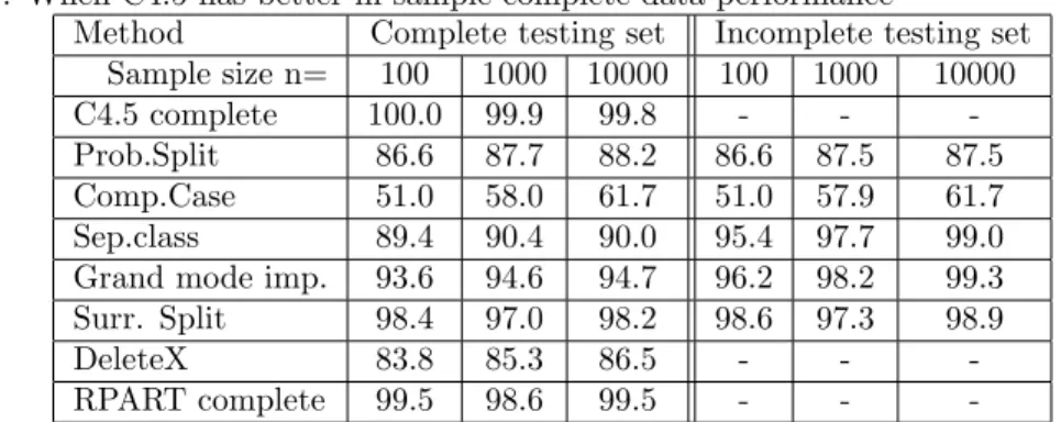
1. When C4.5 has better in sample complete data performance

Method Complete testing set Incomplete testing set Sample size n= 100 1000 10000 100 1000 10000

C4.5 complete 100.0 99.9 99.8 - -

-Prob.Split 86.6 87.7 88.2 86.6 87.5 87.5 Comp.Case 51.0 58.0 61.7 51.0 57.9 61.7 Sep.class 89.4 90.4 90.0 95.4 97.7 99.0 Grand mode imp. 93.6 94.6 94.7 96.2 98.2 99.3 Surr. Split 98.4 97.0 98.2 98.6 97.3 98.9

DeleteX 83.8 85.3 86.5 - -

-RPART complete 99.5 98.6 99.5 - -

-2. When C4.5 andrpart have the same in sample complete data performance Method Complete testing set Incomplete testing set

Sample size n= 100 1000 10000 100 1000 10000

C4.5 complete 93.8 57.9 50.7 - -

DeleteX 80.1 53.9 50.5 - -

-RPART complete 93.8 57.9 50.7 - -

-3. When C4.5 has worse in sample complete data performance

Method Complete testing set Incomplete testing set Sample size n= 100 1000 10000 100 1000 10000

C4.5 complete 76.4 79.7 83.8 - -

DeleteX 68.1 66.1 65.2 - -

-RPART complete 99.7 99.5 99.6 - -

-Table 2: Comparing training set accuracy and new data accuracy. The entries are the percentages of the Monte Carlo replications where training set accuracy is greater than new data set accuracy. Shown in the table are the results from simulations with twelve continuous predictors and six of them subject to missing values.

(16)

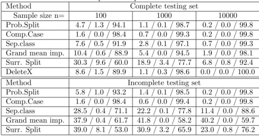
1. When C4.5 has better complete data performance

Method Complete testing set

Sample size n= 100 1000 10000

Prob.Split 4.7 / 1.3 / 94.1 1.1 / 0.1 / 98.7 0.2 / 0.0 / 99.8 Comp.Case 1.6 / 0.0 / 98.4 0.7 / 0.0 / 99.3 0.2 / 0.0 / 99.8 Sep.class 7.6 / 0.5 / 91.9 2.8 / 0.1 / 97.1 0.7 / 0.0 / 99.3 Grand mean imp. 10.4 / 0.6 / 88.9 5.4 / 0.0 / 94.5 1.9 / 0.0 / 98.1 Surr. Split 30.3 / 9.6 / 60.0 18.9 / 3.4 / 77.7 6.8 / 0.8 / 92.4 DeleteX 8.6 / 1.5 / 89.9 1.1 / 0.3 / 98.6 0.0 / 0.0 / 100.0

Method Incomplete testing set

Prob.Split 5.8 / 1.0 / 93.2 1.4 / 0.1 / 98.5 0.2 / 0.0 / 99.8 Comp.Case 1.6 / 0.0 / 98.4 0.6 / 0.0 / 99.4 0.2 / 0.0 / 99.8 Sep.class 28.5 / 0.4 / 71.1 22.2 / 0.1 / 77.8 11.4 / 0.0 / 88.6 Grand mean imp. 37.9 / 0.4 / 61.7 41.8 / 0.0 / 58.2 40.2 / 0.0 / 59.7 Surr. Split 39.0 / 8.1 / 53.0 30.9 / 3.2 / 65.9 23.0 / 0.8 / 76.2 2. When C4.5 and RPART have the same complete data performance

Prob.Split 7.7 / 39.2 / 53.1 2.7 / 86.3 / 11.0 1.1 / 96.9 / 2.0 Comp.Case 6.6 / 26.1 / 67.3 29.0 / 41.3 / 29.7 28.7 / 51.5 / 19.7 Sep.class 26.9 / 33.9 / 39.1 37.7 / 53.4 / 8.9 38.2 / 59.6 / 2.2 Grand mean imp. 31.0 / 33.8 / 35.2 40.8 / 52.3 / 6.9 40.1 / 58.8 / 1.1 Surr. Split 27.9 / 33.4 / 38.7 31.5 / 60.8 / 7.7 23.8 / 74.1 / 2.1 3. When C4.5 has worse complete data performance

Prob.Split 16.6 / 50.8 / 32.6 7.5 / 43.3 / 49.2 6.1 / 29.2 / 64.7 Comp.Case 12.7 / 32.2 / 55.1 14.8 / 21.6 / 63.6 11.1 / 15.2 / 73.7 Sep.class 48.6 / 29.8 / 21.6 41.9 / 26.6 / 31.5 38.4 / 18.7 / 42.9 Grand mean imp. 52.9 / 29.2 / 17.9 49.3 / 25.9 / 24.8 48.3 / 18.2 / 33.5 Surr. Split 27.1 / 4.4 / 68.5 21.6 / 1.4 / 76.9 16.4 / 0.1 / 83.6 Table 3: Comparing relative training set accuracy and relative new data ac-curacy. The entries are the percentages of the Monte Carlo replications where relative training set accuracy is greater than/equal to/less than relative new data accuracy. Shown in the table are results from simulations with twelve

(17)

P P P 100 500 2000 10000 0 20 40 60 80 000 Sample size

Winning pct of each method

C C C S S S M M M T T T D D D P P P 100 500 2000 10000 0 20 40 60 80 001 Sample size

C C C S S S M _M _M T T T D D D P P P 100 500 2000 10000 0 20 40 60 80 010 Sample size

C C C S S S M M M T _T T D D D

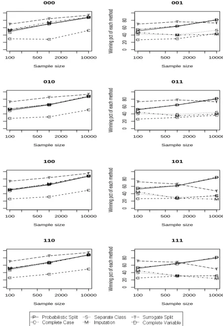
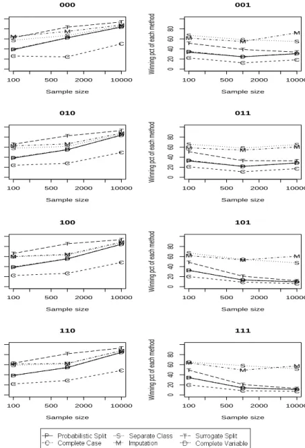
Figure 4: A summary of the order of six missing data method in terms of the relative complete training set accuracy (tested on the complete training set itself). The Y axis is the percentage of times each method is the best (can be tied with other methods). Shown are the results when C4.5 andrpart have the same in sample complete data performance, with twelve continuous predictors and six of them subject to missing values. The three digits indicate if the missingness is dependent on the missing values, on other predictors and on the target variable, respectively, with 0 meaning independent and 1 meaning dependent.

(18)

P P P 100 500 2000 10000 0 20 40 60 80 000 Sample size

C C C S S S M M M T T _T D D D P P P 100 500 2000 10000 0 20 40 60 80 010 Sample size

C C C S S S M _M M T T T D D D P P P 100 500 2000 10000 0 20 40 60 80 100 Sample size

C C C S S S M M M T T T D D D P P _P 100 500 2000 10000 0 20 40 60 80 101 Sample size

C C C S S S M M M T T T D D _D P P P 100 500 2000 10000 0 20 40 60 80 110 Sample size

C C C S S S M M M T T T D D D P P _P 100 500 2000 10000 0 20 40 60 80 111 Sample size

C C C S S S M M M T T T D D _D

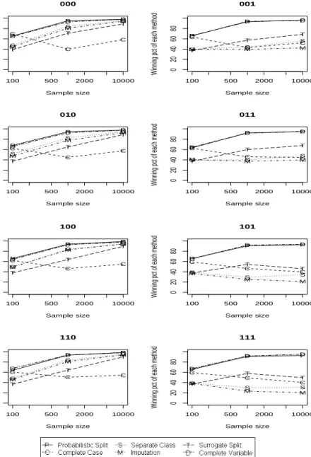
Figure 5: A summary of the order of six missing data method in terms of the relative incomplete training set accuracy (tested on the incomplete training set itself). The Y axis is the percentage of times each method is the best (can be tied with other methods). Shown are the results when C4.5 andrpart have the same in sample complete data performance, with twelve continuous predictors and six of them subject to missing values. The three digits indicate if the missingness is dependent on the missing values, on other predictors and on the target variable, respectively, with 0 meaning independent and 1 meaning dependent.

(19)

P P P 100 500 2000 10000 0 20 40 60 80 000 Sample size

C C C S S S M_T M M T T D D D P P P 100 500 2000 10000 0 20 40 60 80 010 Sample size

C C C S S S MT _M M T T D D D P P P 100 500 2000 10000 0 20 40 60 80 100 Sample size

C C C S S S M M _M T T T D D D P P P 100 500 2000 10000 0 20 40 60 80 110 Sample size

C C C S S S M M M T T T D D D

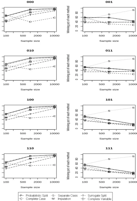
Figure 6: A summary of the order of six missing data method in terms of the relative complete new testing set accuracy (tested on a new complete testing set). The Y axis is the percentage of times each method is the best (can be tied with other methods). Shown are the results when C4.5 andrpart have the same in sample complete data performance, with twelve continuous predictors and six of them subject to missing values. The three digits indicate if the missingness is dependent on the missing values, on other predictors and on the target variable, respectively, with 0 meaning independent and 1 meaning dependent.

(20)

P P P 100 500 2000 10000 0 20 40 60 80 000 Sample size

C C _C S S S MT MT MT D D D P P P 100 500 2000 10000 0 20 40 60 80 010 Sample size

C C C S S S M M M T T T D D D P _P P 100 500 2000 10000 0 20 40 60 80 011 Sample size

C C _C S S S M M M T T T D D D P P P 100 500 2000 10000 0 20 40 60 80 100 Sample size

C C C S S S M M M T T T D D D

Figure 7: A summary of the order of six missing data method in terms of the relative incomplete new testing set accuracy (tested on a new incomplete testing set). The Y axis is the percentage of times each method is the best (can be tied with other methods). Shown are the results when C4.5 andrpart have the same in sample complete data performance, with twelve continuous predictors and six of them subject to missing values. The three digits indicate if the missingness is dependent on the missing values, on other predictors and on the target variable, respectively, with 0 meaning independent and 1 meaning dependent.

(21)

patterns can be clearly seen in Figures 4 to 7 (these figures refer to the case with twelve continuous predictors, six of which are subject to missing values, but results for other situations were broadly similar). In the pictures, the three digits indicate if the missingness is dependent on the missing values, on other predictors and on the target variable, respectively, with 0 meaning independent and 1 meaning dependent. Hence, the left column in the pictures shows the results when the missingness is independent of the target variable and the right column shows the results when the missingness is dependent on the target vari-able. We can see that there are clear difference between the two columns, but within each column there is essentially no difference.

Another clear observation is that the relative performance of all of the miss-ing data methods is very different dependmiss-ing on whether or not there are missmiss-ing values in the testing set. This is detailed in the summary later.

In the following, we first summarize the results when the training set (either the original complete training set or the one containing missing values) is used in the testing phase. These results show the effect of the missing data on the classification trees’ ability to find patterns in the original training data. Also, by treating the pattern in the training data as the “true” DGP/MGP, these results can be thought of as a bridge between expected performance (where is no devia-tion from true DGP/MGP) and the real life situadevia-tion (where deviadevia-tion from the true DGP/MGP exists in both the training set and the testing set). We then summarize the results when a new testing set is used (either complete or with missing values). These results have direct implications in terms of the predic-tive ability of trees when applied to new data. Technically, the only difference between using the training set as the testing set and using a newly generated testing set is the existence of the deviation from the underlying DGP/MGP when a new testing set is used. The deviation from the true DGP/MGP is a potential confounding factor, but by making comparisons between the results of these two situations, its impact can be isolated and this will help us gain a more solid understanding of the effect of the missing data and other factors. As will be seen, the impact of the deviation is in general not important. That is, the patterns in the results are fairly consistent whether the training set or a new data set is used as the testing set. Therefore, the patterns can be attributed to the missing values.

Using the training set as testing set :

1. Complete training set (ref. Figure 4):

• Missingness does not depend on the target variable:

In theory, the complete case method can eventually recover the DGP if the missingness does not depend on the target variable and there are no missing data in the testing set. However, sim-ulations show that this requires a very large sample size. In the simulations, even when there are only eight binary predictors (implying 28_{= 256 cells if the data are partitioned to the finest}

(22)

level) and with sample size 10,000 (giving roughly 40 observa-tions per cell), the complete case method has the worst perfor-mance. The relative performance of the complete case method gets even worse with more predictors or continuous predictors. Since there are no missing data in the testing set, the rules built by the separate class method and applied in the testing phase are only the ones based on complete observations. However, at the training phase, with the extra class in the data, the information gain calculated by the separate class method and the complete case method are different. This may lead to different trees, and thus these two methods will not have same performance. The simulations show that the separate class method tends to have better performance than the complete case method when the sample size is small. Their performances becomes more similar as the sample size gets large.

The complete variable method consistently has the second worst performance. The difference in performance from other meth-ods is relatively smaller when there are more predictors or with continuous predictors, which makes intuitive sense, since in those cases, the loss due to deleting the missing variable(s) is relatively smaller.

Whenrpartand C4.5 have the same complete data performance, surrogate split has the best performance. Its advantage over the other methods is larger when the number of predictors increases. This is probably because the algorithm is more likely to find a good surrogate when there are more predictors to choose from, and thus surrogate split is more likely to perform better. The relative performances of all of the other methods are the same with or without surrogate split in the picture. When all of the predictors are binary, the imputation method has the second best performance, but the edge over the other methods is small. However, with continuous predictors, all of the methods except for the complete case method (the worst) have very similar per-formance. The performance of all of the missing data methods becomes more similar as sample size grows.

• Missingness depends on the target variable:

In this case, probabilistic split appears to have the best per-formance. This is consistent with the simulated 2×2 table re-sults. When the predictors are continuous, the complete vari-able method has a comparvari-able performance. This is probably because it is not too difficult to pick up the lost information in the deleted predictor from the remaining continuous predictors (in the simulation, there are always three remaining predictors that are correlated with the deleted one(s)). When surrogate split is comparable (i.e. rpart and C4.5 have the same complete

(23)

data performance), its performance is slightly worse than that of probabilistic split.

As was noted earlier, separate class should have similar behavior as the complete case method. Not surprisingly, in the simula-tions, the separate class method has the second worst perfor-mance, only better than the complete case method.

2. Incomplete training set (ref. Figure 5):

Consistent with previous analysis, when the missingness depends on the target variable, it is obvious that the separate class method is the dominantly best performer. This is especially true with binary predictors.

When the predictors are continuous, the imputation method is comparable to separate class and sometimes even better. This is because when the predictor is continuous, the imputed mean is likely to be different from the existing values and effectively creates a “separate class”. The fact that this “separate class” is reasonably in line with the data, unlike the very large (or small) value used in the separate class method, probably gives it an advantage over the separate class method. This is not the case for mode imputation with categorical predictors, because the imputed mode is one of the existing categories and not a “separate class”.

The same pattern holds even if the missingness does not depend on the target variable. This is presumably due to the fact that the training set itself is used as the testing set. In this case, even though the missingness and the target variable are indeed independent, they are likely to have some relationship in the training set just by chance alone. The separate class method can pick up this “relationship” in the training set. Even though the “relationship” is just random fluctuation, it still exists in the testing set (since the testing set is the training set), and therefore the separate class method can benefit from it.

The complete case method, the complete variable method and probabilistic split have the worst performance. Probabilistic split attempts to mix the observations with missing values into the complete ones, and as a result does not use the “information” in the missingness effectively. However, the performance of all of the missing data methods becomes more similar as sample size grows.

Using a new data set as testing set :

As we have mentioned, by using a newly generated data set as the testing set, random deviation from the underlying DGP/MGP is introduced into

(24)

the simulation. It turns out that the impact of the deviation is generally small, and the patterns in the results are similar to those when the training set is used as the testing set. In the following summary, we will omit the detailed explanation when it is the same as when the training set is used as the testing set.

1. Complete new data (ref. Figure 6):

The complete case method can only recover the DGP with a very large average sample size when the missingness is independent of the target variable. When the complete data performance of rpart is comparable, surrogate split does not seem to have an advantage over other methods; its better complete training set performance is likely due to over fitting of the original data. There is no clear winner when the predictors are binary. The complete variable method and the separate class method seem to be a little worse than the others. When the predictors are continuous, however, probabilistic split seems to be the best. The complete variable method has the second best performance and is comparable to probabilistic split with continuous predictors, presumably for the same reason as when the training set is used as the testing set (that the remaining continuous predictors can compensate for the lost information in the deleted ones). The performance of all of the missing data methods becomes more similar as the sample size grows.

Similar to the complete training set case, when the missingness depends on the target variable probabilistic split seems to be the best. The complete variable method has the second best perfor-mance and is comparable to probabilistic split with continuous predictors, presumably for the same reason as given before (that the remaining continuous predictors can compensate for the lost information in the deleted ones).

2. Incomplete new data (ref. Figure 7):

The separate class method is the obvious dominant one when the missingness depends on the target variable. When predictors are continuous, the imputation method no longer has compara-ble performance. The reason is that the imputed mean in the training set is likely to be different from the imputed mean in the testing set, and the pattern for this “separate class” learned from the training set is not helpful in the testing phase. This re-inforces that the creation of a “separate class” that is predictive for the target variable is the key aspect in the gains in predictive power.

(25)

When the missingness does not depend on the target variable, the results are almost identical to the situation with complete new testing set. That is, there is no clear winner when the predictors are binary, but if the predictors are continuous then probabilis-tic split and the complete variable method seem to have the best performance. In this case, there is no information about the tar-get variable in the missingness, and therefore the mix-in strategy of probabilistic split and the “ignore-it” strategy of the complete variable method may be slightly better than trying to force the gain out of the no-information missingness (as in separate class). The performance of all of the missing data methods becomes more similar as sample size grows.

Surrogate split has a slightly better in sample performance compared to predictive performance when the predictors are binary and there are complete predictors that are strongly related to the missing ones, but otherwise its perfor-mance is unrelated to the strength of the association between the variable with missing data and the other predictors. This might seem surprising (since an uncorrelated surrogate would seem to have less success “replacing” the missing variable), but since surrogate split works operates at the level of each node a global measure of the strength between the predictors (e.g. correlation) might not be a good indicator of its expected performance. Another possible explana-tion is that the sample size at each node is too small for surrogate split to work efficiently even when it would be expected to be effective.

5 A REAL DATA EXAMPLE

We now present a real data example. In this example, we try to predict a company’s bankruptcy status given its key financial statement items. The data are annual financial statement data and the predictions are sequential. That is, we build the tree on one year’s data and then test its performance on the following year’s data. For example, we build a tree on 1987’s data and test its performance on 1988’s data, then build a tree on 1988’s data and test it on 1989 data, and so on.

The data are retrieved from Compustat North America (a database of U.S. and Canadian fundamental and market information on more than 24,000 active and inactive publicly held companies). Following Altman and Sabato (2005), twelve variables from the data base are used as potential predictors: Current Assets, Current Liabilities, Assets, Sales, Operating Income Before Deprecia-tion, Retained Earnings, Net Income, Operating Income After DepreciaDeprecia-tion, Working Capital, Liabilities, Stockholder’s Equity and year. The target vari-able, bankruptcy status, is determined using two footnote variables, the footnote

(26)

for Sales and the footnote for Assets. Companies with remarks corresponding to “Reflects the adoption of fresh-start accounting upon emerging from Chap-ter 11 bankruptcy” or “Company in bankruptcy or liquidation” are marked as bankruptcy. The data include all active companies, and span 19 years from 1987 to 2005. There are 177560 observations in the original retrieved data, but 76504 of the observations have no data except for the company identifications, and are removed from the data set, resulting in 99056 observations. There are 19238 observations containing missing values and there are 56820 missing data values.

According to the results in Section 4, there are two criteria that differentiate the performance of different missing data methods, i.e. whether or not there are missing values in the testing set and whether or not the missingness depends on the target variable. In the bankruptcy data, there are missing values in every year’s data, and thus missing values in each testing data set. To assess the dependence of the missingness on the target variable, the following test is carried out. First, define twelve new binary missingness indicators corresponding to the original twelve predictors. The indicators take on value 1 if the original variable is missing and 0 if the original value is observed for that observation. We then build a tree for each year’s data using the indicators as the predictors and the original target variable, the bankruptcy status as the target variable. From 1987 to 2000, the tree makes no split, indicating the target variable is not strongly related to the indicators (that is, missingness does not seem to carry enough information about the bankruptcy status). From 2001 to 2005, the classification tree consistently splits on the missingness indicators of Sales and Retained Earnings. This indicates that the missingness of these predictors has clear information about the target variable in these years, and the MGP across the years is fairly consistent in missingness in sales and retained earnings being related to bankruptcy status.

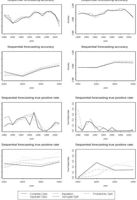
Given these observations and the fact that the sample sizes are fairly large, we would make the following propositions based on our earlier conclusions. First, from 1988 to 2001 (since the tree tested on 2001 data is built on 2000 data), different missing data methods should have similar performance, with no clear winners. However, from year 2002 to year 2005, the separate class method should have the best performance. The actual relative performance of different missing data methods is shown in Figure 8. Since surrogate split is realized usingrpartwhile probabilistic split is realized using C4.5, we run all of the other methods using bothrpartand C4.5 so that we can compare both surrogate split and probabilistic split with all of the other methods. In Figure 8, the plots on the left are the results fromrpart, which include all of the missing data methods except for probabilistic split. The plots on the right are the results from C4.5, which include all of the missing data methods except for surrogate split. The performances of methods common to both plots are slightly different because of differences between C4.5 andrpart in splitting and pruning rules. Both the accuracy and the true positive rates are shown. Since the number of actual bankruptcy cases in the data is small, the accuracy is always very high. The

(27)

true positive rate is defined as

T P =Number of correctly predicted bankruptcy cases Actual number of bankruptcy cases .

The graphs in the first and the second rows are for accuracies, with the first row for the first time period from 1988 to 2001 and the second row for the second time period from 2002 to 2005. The graphs in the third and the fourth rows are for true positive rates, with the third row for the first time period from 1988 to 2001 and the fourth row for the second time period from 2002 to 2005. It is apparent that in the first time period, there are no clear winners. However, in the second time period, separate class almost always has the best performance, in line with expectations.

6 CONCLUSION AND FUTURE STUDY

We have shown that depending on the testing set (whether or not it contains missing values), different missingness patterns in predictor variables (does or does not depend on the target variable) can have a strong effect on the effec-tiveness of classification trees. That is, the two most important criteria that differentiate the performance of different missing data methods are whether or not the testing set is complete and whether or not the missingness depends on the target variable. The analytical results and simulations imply the following. 1. Deleting the observations that contain missing values is in general not a good approach. The only exception is when the sample size is very large relative to the number of predictors (at least larger than 40 observations per leaf node) and the missingness is independent of the target variable and also the testing set is complete. In this case, by using only the complete cases, the tree is expected to recover the underlying DGP.

If the sample size is large but not enough for the complete case method to perform as expected, imputation and separate class tend to have better performance than the other methods. But as the sample size decreases, the relative performance of these two methods deteriorates and the advantage shifts to probabilistic split.

2. When the missingness is independent of the target variable and there isn’t a very large sample size, or if the missingness is dependent on the target variable and the testing set is complete, then probabilistic split is a good choice. If there is a large number of predictors and the completely observed ones can pick up the information in the ones containing missing values, then ignoring the missing predictors may also be a good idea.

3. When the missingness is dependent on the target variable and the test-ing set also contain misstest-ing values, then treattest-ing the misstest-ing values as a separate class is clearly the best method.

(28)

Sequential forecasting accuracy year Accuracy 1988 1990 1992 1994 1996 1998 2000 0.980 0.990 1.000

Sequential forecasting accuracy

year Accuracy 1988 1990 1992 1994 1996 1998 2000 0.980 0.990 1.000

year Accuracy 2002 2003 2004 2005 0.980 0.990 1.000

Sequential forecasting true positive rate

year

True Positive Rate

1988 1990 1992 1994 1996 1998 2000 0.0 0.1 0.2 0.3 0.4 0.5

year

True Positive Rate

1988 1990 1992 1994 1996 1998 2000 0.0 0.1 0.2 0.3 0.4 0.5

year

True Positive Rate

2002 2003 2004 2005 0.0 0.1 0.2 0.3 0.4 0.5

year

True Positive Rate

2002 2003 2004 2005 0.0 0.1 0.2 0.3 0.4 0.5

Figure 8: The relative performance of all of the missing data methods on the bankruptcy data. The left column are methods usingrpart (includes all of the methods except for probabilistic split) and the right column are methods using C4.5 (includes all of the methods except for surrogate split). The top row are performances in terms of accuracy while the bottom row are in terms of true positive rate.

(29)

Classification trees are designed for the situation where the target variable is categorical, not just binary; it would be interesting to see how these results carry over to that situation. Tree-based methodologies for the situation with a numerical target have also been developed (i.e. regression trees), and the prob-lems of missing data occur in that context also. A weakness of the simulations is that the DGP and MGP are specified by the researcher; further analysis of real data, where the DGP and MGP occur naturally, is needed. Given the results here, it could be expected in each of these cases that a key aspect of tree algo-rithm effectiveness would be whether missingness depends on the target, rather than the MAR/MCAR/NMAR structure of the missingness.

7 APPENDIX: PROOFS OF THE

THEOREMS

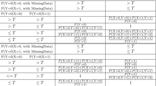
The relative accuracy (RelAcc) when there are missing values in the train-ing set but not in the testtrain-ing set can be summarized into Table 4, where T is the threshold value (an observation will be classified as class 0 if the pre-dicted probability for it to be 0 is greater than T). The value of T reflects the misclassification cost. It is taken as 0.5 reflecting a equal misclassification cost. In Table 4, the columns show different rules given by the classification trees when there are missing values and the rows show actual DGP’s. The entries are theRelAccs under different scenarios. For example, all the entries on the diagonal are one’s because the rules given by the classification trees when there are missing values are the same as the true DGP’s and thus the accuracy achieved by the trees are the same with or without the missing val-ues and thusRelAcc = 1. Cell of row 1 and column 2 shows that if the true DGP isP(Y = 0|X = 0) > T and P(Y = 0|X = 1) > T but the classifica-tion tree gives rule P(Y = 0|X = 0) > T and P(Y = 0|X = 1) ≤ T when there are missing values, i.e. P(Y = 0|X = 0,with missing value) > T and P(Y = 0|X = 1with missing value) ≤ T, then the relative accuracy is dter-mined to be

P(X = 0, Y = 0) +P(X = 1, Y = 1)

P(Y = 0) .

Proof of Theorem 1 : The expected performance of the complete case method when the missingness does not depend on the target variable and the test-ing set is complete.

Proof. If only the complete cases are used, if P(Y|A= 0, X) =P(Y|X), then only the diagonal in Table 4 can be achieved, and thus there is no loss in accuracy. Ais the case-wise missingness indicator which equals 1 if the observation contains missing values in one or more of the predictors or 0