Sample- and segment-size specific Model Selection in Mixture Regression Analysis

(1)

Sample- and segment-size specific Model Selection in Mixture

Regression Analysis

A Monte Carlo simulation study Marko Sarstedt

Discussion Paper 2006-8 November 2006

LMU

LUDWIG-MAXIMILIANS-UNIVERSITÄT MÜNCHEN

MUNICH SCHOOL OF MANAGEMENT

(2)

Abstract

As mixture regression models increasingly receive attention from both theory and practice, the question of selecting the correct number of segments gains urgency. A misspecification can lead to an under- or oversegmentation, thus resulting in flawed management decisions on customer targeting or product positioning.

This paper presents the results of an extensive simulation study that examines the performance of commonly used information criteria in a mixture regression context with normal data. Unlike with previous studies, the performance is evaluated at a broad range of sample/segment size combinations being the most critical factors for the effectiveness of the criteria from both a theoretical and practical point of view. In order to assess the absolute performance of each criterion with respect to chance, the performance is reviewed against so called chance criteria, derived from discriminant analysis.

The results induce recommendations on criterion selection when a certain sample size is given and help to judge what sample size is needed in order to guarantee an accurate decision based on a certain criterion respectively.

(4)

1. Introduction

Finite mixture models have been applied in various research fields for more than a century now. These research fields include astronomy, biology, genetics, psychology, engineering criminology and marketing (MCLACHLAN/PEEL 2000; TITTERINGTON ET AL.1985). Especially

in the latter, finite mixture models have recently received increasing attention from both a practical and theoretical point of view. In the last years, traditional mixture models have been extended by various multivariate statistical methods such as multidimensional scaling, exploratory factor analysis (DESARBO ET AL.2001a) or structural equation models (JEDIDI ET AL. 1979; HAHN ET AL.2002), upon which regression models (WEDEL/KAMAKURA 1999,pp.

99) for normally distributed data are the most common analysis procedure in marketing context, e.g. in terms of conjoint and market response models (ANDREWS ET AL. 2002;

ANDREWS/CURRIM 2003b, p.316). Correspondingly, mixture regression models are prevalent

in marketing literature (BOWMAN ET AL. 2004; DESARBO ET AL. 2001b; SRINIVASAN 2006;

REINARTZ ET AL. 2005; SJOQUIST ET AL. 2003; WEDEL/DESARBO 2002; YOO 2003 among

others) and are expected to become more and more common as recent research suggests that finite mixture conjoint models produce good parameter estimates, even at an individual level (ANDREWS ET AL. 2002b).

Despite their widespread use and the importance of retaining the true number of segments in order to reach meaningful conclusions from any analysis, determining the true number of segments is still an unresolved problem (ANDREWS/CURRIM 2003a, p. 235;

WEDEL/KAMAKURA 1999, p. 91). A misspecification can lead to an under- or

oversegmentation, thus leading to flawed management decisions on e.g. customer targeting, product positioning or the determination of the optimal marketing mix (ANDREWS/CURRIM

2003a, p. 235).If the number of segments is over-specified, marketers may run the risk of treating audience segments separately even though they could be handled together more effectively. On the other hand, if a market is under-segmented, marketers may miss out on identifying distinct segments that could be addressed separately for more precise satisfaction of the customer’s varying wants. DILLON andKUMAR state in this context that “the challenges

that lie ahead are […] falling squarely on the development of procedures for identifying the number of support points needed to characterize the components of the mixture distribution under investigation” (DILLON/KUMAR 1994,p.345). Therefore the objective of this paper is to

give recommendations on which criterion should be considered at what combination of sample/segment size in order to identify the true number of segments in a given data set.

(5)

Various authors have considered the problem of choosing the number of segments in mixture models in different context (see BOZDOGAN 1993;BRAME ET AL.2006;CELEUX/SOROMENHO

1996; CUTLER/WINDHAM 1993; MCLACHLAN/NG 2000; NYLUND ET AL. 2006; RUST ET AL.

1995; SOROMENHO 1993;TOFIGHI/ENDERS 2007;YANG 2006 among others). But as most of

the available studies appeared in statistics literature, they aim at exemplifying the effectiveness of new proposed measures, instead of revealing the performance of measures commonly available in statistical packages. Despite its practical importance, this topic has not been thoroughly considered for mixture regression models.

An exception in this area are the studies by HAWKINS ET AL. (2001), ANDREWS/CURRIM

(2003b)andOLIVEIRA-BROCHADO/MARTINS (2006),who examine the performance of various

information criteria against several factors such as measurement level of predictors, number of predictors, separation of the segments or error variance. Although sample and segment size are critical factors, from both a practical as well as theoretical point of view (will be clarified later), their interaction is not thoroughly considered in previous studies. Unlike the mentioned articles, this paper aims at filling this gap by determining how the interaction of sample and segment size affects the performance of five of the most widely used criteria for assessing the number of segments in mixture models in detail. To do so, a Monte Carlo simulation was conducted for a two-segment solution where the sample size was varied in a ten-step interval of [50;500]. For each sample size, five variations of mixture proportions were evaluated. In order to assess the relative performance of each criterion, success rates for choosing the right number of segments were computed.

Another shortcoming of existing studies is their plain focus on the criteria’s relative effectiveness, ignoring any a-priori information on the likelihood with which a certain model may occur. As a consequence, the success rates of the simulation were compared with an outside criterion, so called chance models, derived from discriminant analysis, in order to evaluate the criteria’s absolute performance with respect to chance.

The rest of the article proceeds as follows:

The next section contains the necessary theoretical background on mixture regression models and a short review of model selection criteria. In order to identify commonly used information criteria, a meta-study on the utilization of statistical figures for model selection was conducted whose results are presented in this section. Then, the design of the simulation study is introduced, followed by the results of the study. Finally, the study’s resulty, as well as management implications and suggestions for further research are presented.

(6)

2. Theoretical Background

2.1 Mixture Regression Models

A mixture model based approach to regression assumes that the observations of a data set originate from various groups with unknown segment affiliations. This heterogeneity is treated in simultaneous equation models by deriving segments that are homogenous in respect to predictor values of the model. That is, each observation is taken to be a realization of the unconditional density

(

_{) ∑}

= ⋅ = K i i n i i n f y y f 1 ) | ( |φ π θ (1)

withφ =

(

πi,θi

)

, yn as the dependent variable (n=1,…,N), πi as the mixture proportion of

segment i ( ) and as the vector of all

unknown parameters associated with the density function where

K 1,..., i 0 and 1 i 1 = ∀ ≥ =

∑

= π π K i i

(

′ ′ ′ = π1,...,π_K;θ1,...,θ_K φ

)

i θ is the segment-specific parameter vector for the density function. Equation (1) describes a mixture linear regression (also latent class regression or cluster-wise regression) if the conditional density function is a normal density with the segment-specific mean

i f x i β′ and variance 2 i σ .

Applications of mixture regression models are typically classified according to the distribution of the dependent variable (WEDEL/KAMAKURA 1999, p. 113). The most important

distributions are normal, gamma or exponential for continuous variables and binomial, multinomial or Poisson for discrete variables. As all these distribution types are within the exponential family, generalized linear models can be applied, including linear regression, logit or probit models. Other models include censored regression models, such as the tobit model or survival models, such as the Cox Proportional Hazards Model (COX 1972).

2.2 Model Selection in Mixture Models

Assessing the number of segments in a mixture model is a difficult but important problem. Whereas it is well known that conventional chi square-based goodness of fit tests and likelihood ratio tests are unsuitable for making this determination (AITKIN/RUBIN 1985;

EVERITT 1981;EVERITT 1988), the decision on what model selection statistic should be used

still remains unsolved (MCLACHLAN/PEEL 2000, pp. 175; NYLUND ET AL. 2006, pp. 4). A

modified likelihood ratio test (MCLACHLAN 1987) uses bootstrapping procedures to

circumnavigate implementation problems of classical chi square tests but requires vast computing power (WEDEL/KAMAKURA 1999, p. 91). To date this so called bootstrap

(7)

therefore lacks general application. The more recently developed Lo-Mendell-Rubin test (LO ET AL. 2001) compares two neighbouring models and provides a p-value to contrast the

increase in model fit between k-1 and k class models by using an approximate reference distribution for the log likelihood difference. However, this method has been criticized by JEFFRIES (2003) due to analytic inconsistency, which questions the validity of testing

non-nested models with this method.

The other main approach for deciding on the number of segments is based on a penalized form of the likelihood, yielding to the so called information criteria. Information criteria for model selection simultaneously take into account the goodness-of-fit (likelihood) of a model and the number of parameters used to achieve that fit. They therefore correspond to a penalized likelihood function, that is, the negative likelihood plus a penalty term, which increases with the number of parameters and/or the number of observations. Various model selection criteria which take the form

[

max ( )

]

( ) ( ) ( , ) ln

2 L k +a n m k +b k n

− (2)

have been developed in recent years. Here, n is the sample size, max L(k) denotes the maximum of the likelihood over the parameters, and m(k) is the number of independent parameters in a model with k segments. For a given criterion, a(n) is the cost of fitting an additional segment and b(k,n) is an auxiliary term depending upon the criterion. According to these criteria, among a set of competing models the model minimizing the value in equation (2) should be chosen.

The simulation study focuses on four of the most representative and widely applied models selection criteria. In a recent study byOLIVEIRA-BROCHADO and MARTINS (2006), the authors

report that in 37 published studies, AIC was used 15 times, CAIC was used 13 times and BIC was used 11 times (multiple selections possible). Since it remains unclear in which publications the studies appeared, an own meta-study was initiated in order to identify the most commonly used information criteria in the field of marketing. For this purpose, all marketing journals rated A or A+ in both rankings, developed on behalf of the Vienna University of Economics and Business Administration in 2001 and the Association of University Professors of Management in German speaking countries (VHB) in 2003 (for a complete list, cp. HARZING 2006) were considered.

In order to make the data construction as transparent as possible, an easily accessible but universal research database was used. In November 2006, EBSCO was searched for any

(8)

reference to “finite mixture”, “mixture regression” and “latent regression”. EBSCO is the most comprehensive full text database for peer-reviewed research papers.

The EBSCO search led to a great number of references of which a large fraction covered an entirely different topic. The empirical papers were examined whether they actually used any type of mixture regression analysis. Eventually, the desired results could be gained from 33 articles that appeared between January 2000 and November 2006.

One paper was discarded from the analysis due to missing specifications on the model selection statistic used. In the remaining 32 articles, the problem of model selection and the decision for an appropriate statistical figure is only addressed four times: DANAHER/MAWHINNEY (2001), DANAHER (2002) and WU/RANGASWAMY (2003) refer to a

contribution by BUCKLIN/GUPTA (1992) who apply multiple-segment choice models to

capture customer heterogeneity in brand choice. In this study, the authors briefly discuss the advantageousness of likelihood ratio tests, the Akaike’s Information Criterion (AIC) and the Bayesian Information Criterion (BIC) from a theoretical point of view without referring to any simulation study results. Only ANDREWS ET AL. (2002a) give detailed reasons for their

selection of the model selection criteria. This decision is based on the, at that time unpublished, study “A Comparison of Segment Retention Criteria for Finite Mixture Logit Models” (ANDREWS/CURRIM 2003a). In the remaining 28 studies, no rationale whatsoever is

given for the model selection statistics chosen. In none of the studies did the authors draw back on test statistics to decide on the number of segments in the mixture. In fact, all authors refer to information criteria to make that decision. In the studies, BIC was used 25 times, AIC was used eight times and Consistent Akaike’s Information Criterion (CAIC) as well as Modified AIC with factor three (MAIC3) was used two times (multiple selections possible). In six cases more than one information criterion was applied.

In four cases, the log-marginal density (LMD), which is computed as the logarithm of the harmonic means of the likelihood values is used as an in-sample fit criterion. Because the likelihood values are obtained using the estimated parameter samples drawn by Gibbs sampling which is not applicable in this context, the LMD criterion is not considered in this study. For a summary of the meta-study, see the Appendix.

With regard to application statistical computing software, one can observe that the criteria mentioned are also implemented into widely used software alternatives for estimating mixture models such as FlexMix (LEISCH 2004; GRÜN/LEISCH 2006a; GRÜN/LEISCH 2006b: AIC,

(9)

BIC), Latent Gold (VERMUNT/MAGIDSON 2005: AIC, BIC, MAIC3, CAIC) or Mplus

(MUTHÉN/MUTHÉN 2006:AIC,BIC,ABIC).

As a consequence, the following criteria were considered: Akaike’s Information Criterion (AIC), Bayesian Information Criterion (BIC), Consistent Akaike’s Information Criterion (CAIC), Sample-size adjusted BIC (ABIC), Modified AIC with factor 3 (MAIC3).

In the course of a number of papers, AKAIKE (1973, among others) developed a criterion as an

estimate of the expected entropy, later introduced in a mixture context by BOZDOGAN and

SCLOVE (1984), which takes the following form:

) ( 2 ln 2 L m k AIC =− ⋅ + ⋅ (3)

The AIC penalizes the log likelihood by the total number of parameters required for model estimation by adding two times the number of degrees of freedom. In addition to the often observed inconsistency (BOZDOGAN 1987; KOEHLER/MURPHEE 1988; WOODROOFE 1982),

numerous authors noticed that the AIC tends to overestimate the true number of segments in mixture models (ANDREWS/CURRIM 2003b; SOROMENHO 1993; CELEUX/SOROMENHO 1996;

MCLACHLAN/NG 2000). Despite the problems associated with the application of this criterion,

it still constitutes the standard in model selection criteria (OLIVEIRA-BROCHADO/MARTINS

2006, p. 2).

Subsequent research took critical remarks on the features of the AIC into account by increasing the penalty term. BOZDOGAN (1994) proposed a penalty term with a(n)=3, consecutively referred to as MAIC3. Furthermore BOZDOGAN (1987) provided the CAIC

which is defined as ] 1 [ln ) ( ln 2⋅ + ⋅ + − = L m k n CAIC . (4)

The criterion imposes a larger penalty term than the AIC that grows with increasing sample size. This makes the CAIC asymptotically consistent, and overparametrization is penalized more stringently (BOZDOGAN 1987, pp.357). Therefore, compared to AIC, the CAIC prefers

models with fewer segments (WEDEL/KAMAKURA 1999, pp.92).

As an alternative to the AIC, SCHWARZ (1978) developed the BIC, which is derived within a

Bayesian framework for model selection and is computed as

) ( ln ln 2 L n m k BIC =− ⋅ + ⋅ . (5)

(10)

Like the CAIC, the BIC penalizes the log likelihood by considering the total number of parameters required for model fit and the total sample size by adding the natural log of the sample size n times the number of degrees of freedom. Just like CAIC, the BIC points to the right model with probability of unity as the sample size increases. MCLACHLAN and PEEL

(2000, pp. 209) point out that for ln n > 2 and n > 8, the penalty term penalizes models stronger than the AIC, reducing the AIC’s tendency to overparametrize models (LEROUX

1992, pp. 1350). However, CUTLER and WINDHAM (1993) show in their simulation study that

the extension of the penalty term can indeed result in an underparametrization, i.e. underestimation of the true number of segments.

In Mplus, one of the most widely used software packages for estimating mixture models, MUTHÉN and MUTHÉN (2006) included the sample-size adjusted BIC, originally derived by

RISSANEN (1978) and suggested by SCLOVE (1987) to work well in mixture models.

The ABIC is described by

) ( 24 2 ln ln 2 L n m k ABIC=− ⋅ + + ⋅ . (6)

Recent developments impose a penalty on the likelihood that is related to other factors. The Information Complexity Criterion (ICOMP), for example, is based on the properties of the (estimated) Fisher information matrix (BOZDOGAN 1990; BOZDOGAN 1993) and shows a

compared to the more traditional criteria AIC and BIC advantageous performance, depending on the context of usage (CUTLER/WINDHAM 1993; ANDREWS/CURRIM 2003a). Other criteria

include the Consistent Akaike’s Information Criterion with Fisher Information (CAICF) (BOZDOGAN 1987, pp. 359), the Efron Information Criterion (EIC) (ISHIGURO ET AL.1997),

the Integrated Completed Likelihood Criterion (ICL) (BIERNACKI ET AL.2000) or the recently

developed New Covariance Ination Criterion (New CIC) by RODRÍGUEZ (2005).1

However, these criteria have not found their way into the widely used software programs described above.

Despite the importance of regression models in marketing context, only two studies so far observe the performance of information criteria in mixture regression models. The study by ANDREWS and CURRIM (2003b) examines the performance of AIC, MAIC3, CAIC, BIC,

ICOMP, the validation sample log likelihood (LOGLV) and the Normed Entropy Criterion (NEC) (CELEUX/SOROMENHO 1996) by counting the success rates of each criterion under

(11)

consideration of the Root Mean Square Error between the true and estimated parameters of the chosen model. The examination is carried out based on simulated data sets with eight factors, which according to literature potentially affect the criteria performance. In every experimental condition, MAIC3 shows the best overall performance, followed by LOGLV and BIC, the latter of which dominates CAIC. At last, AIC showed high overfitting rates and ICOMP low overall success rates. The authors conclude that MAIC3 is the best criterion to use with regression models for normally distributed data. Whereas the study provides good insight into the criteria’s overall performance, it remains unclear in which factor level combination each criterion operates favourably or not. In a simulation studyHAWKINS ET AL.

(2001) consider similar information criteria to those used in the study by ANDREWS and

CURRIM (2003b) and evaluate the influence of segment separation and mixing proportions.

From the criteria mentioned above, ICOMP performed best, followed by MAIC3. But the authors themselves state that the simulation results are limited since the effects of small sample sizes were not explored.

In a more recent study,OLIVEIRA-BROCHADO and MARTINS (2006) examine model selection

criteria performance in recovering small niche segments as well as the impact of distributional misspecification of the error term. The experimental design comprised of data sets with six predictors, an alternating number of segments and mean separations between segment coefficients. In the niche segment case, AIC and AIC with a penalty term of a(n)=3 and a(n)=4 showed the best performance, whereas BIC and CAIC, just like most of the other criteria not presented in this paper showed rather poor performance. Furthermore, it turned out that segment retention criteria did not loose performance with distributional misspecification of the error term which followed a uniform distribution.

Despite the broad scope of questions covered in these studies, they do not profoundly investigate the criteria’s performance against the one factor best influenceable by the marketing analyst, namely the sample size.2 From an application-oriented point of view, it is desirable to know which sample size is necessary in order to guarantee validity when choosing a model with a certain criterion. Furthermore, the disregard of sample size not only proves problematic from a practical but also theoretical point of view. As indicated above, the sample size is a key differentiator between the criteria, because -2ln[max L(k)] from equation (2) remains the same for all criteria, described in equations (3) through (6). Consequently, the sample size must have a large effect on the criteria’s effectiveness, taking into account that

2_{Whereas H}_{AWKINS ET AL}_._{(2001) use a sample size of n=500, O}_LIVEIRA_-B_ROCHADO_{and M}_ARTINS₍₂₀₀₆₎

consider a sample size of n=300 and ANDREWS and CURRIM (2003b) allow two levels of sample sizes (n=100 and n=300).

(12)

available studies yield different conclusions about the advantageousness of their performance. Therefore, the first objective of this study is to determine how well the information criteria perform in mixture regression of normal data, with alternating sample sizes.

Another factor that is closely related to this problem concerns segment size ratio. Even though a specific sample size might prove beneficial in order to guarantee a satisfactory performance of the information criteria in general, the presence of niche segments might lead to a reduced heterogeneity and thus to a wrong decision in choosing the number of segments. That is why the second objective is to measure the information criteria’s performance in order to be able to assess the validity of the criteria chosen when specific segment and sample sizes are present. These factors are evaluated for a two-segment solution.

3. Simulation design

The strategy for this simulation consists of initially drawing observations derived from an ordinary least squares regression and applying these to the FlexMix algorithm (LEISCH 2004;

GRÜN/LEISCH 2006a;GRÜN/LEISCH 2006b) on a previously generated data set. FlexMix is a

general framework for finite mixtures of regression models using the EM algorithm which is available as an extension package for the statistical computing software R (RDEVELOPMENT

CORE TEAM 2006).

In this simulation study, models with alternating observations and three continuous predictors were considered for the OLS regression. First,

i

n

X

β

Y= ′ was computed for each observation, where X was drawn from a normal distribution. Subsequently an error term derived form a standard normal distribution was added to the true values. Each simulation set up was run with 1.000 iterations.

The main parameters controlling the simulation were: The number of segments: K=2

The regression coefficients in each segment which were specified under the premise of setting the mean separation between segment coefficients at 1:

- Segment 1: β1 =

(

1 ,1,1.5,2.5

)

′

- Segment 2: β2 =

(

1 ,2.5,1.5,4

)

′

(13)

For each sample size, the simulation was run for the following five mixture proportions: ( 0.1, 0.9);( 0.2, 2 0.8); 2 2 1 1 2 1 1 = π = π = π = π ( 0.3, 3 0.7); 2 3 1 = π = π )} 5 . 0 , 5 . 0 ( ); 6 . 0 , 4 . 0 ( 5 2 5 1 4 2 4 1 = π = π = π = π

Each simulation run was carried out five times for k=1,…,5 segments.

The likelihood was maximized using the EM algorithm (DEMPSTER ET AL. 1977). As a

limitation of the algorithm is its convergence to local maxima (WEDEL/KAMAKURA 1999, p.

88), it is run repeatedly with 10 replications, totalling in 50 runs per iteration. For each number of segments, the best solution was picked.

4. Results summary

As indicated above, previous studies only observe the criteria’s relative performance, ignoring the question whether the criteria perform any better than chance. To gain a deeper understanding of the criteria’s absolute performance one has to compare the success rates with an ex ante specified chance model. In order to verify whether the criteria are adequate, the predictive accuracy of each criterion with respect to chance is measured using the following chance models derived from discriminant analysis (MORRISON 1969) and represented in the

following graphics: Random chance, proportional chance and maximum chance criterion. In order to be able to apply these criteria, the researcher has to have prior knowledge or make presumptions concerning the underlying model:

For a given data set, let be a model with segments from a consideration set with C competing models

j

M K_j

{

M1,...,MC

}

=

Κ and ρj be the prior probability to observe (j=1,…,C

and

∑

). The random chance criterion is

j M = = C j j 1 1 ρ ρ = = C CMran 1 (7)

which indicates that each of the competing models has an equal prior probability. The proportional chance criterion is

∑

₌ = C j j prop CM 1 2 ρ (8)

(14)

which has been used mainly as a point of reference for subjective evaluation (MORRISON

1969), rather than the basis of a statistical test to determine if the expected proportion differs from the observed proportion of models that is correctly classified.

The maximum chance criterion is

(

C

)

CMmax =max ρ1,...,ρ (9)

which defines the maximum prior probability to observe model j in a given consideration set as being the benchmark for a criterion’s success rate. Since CMran <CMprop <CMmax,

denotes the strictest of the three chance model criteria. If a criterion cannot do better than , one might disregard the model selection statistics and choose where

max CM

max

C M_j max

( )

ρj . But

as model selection criteria may defy the odds by pointing at a model i where ρ_i ≤max

( )

ρ_j , in most situations Cprop should be used.

Relating to the focus of this article, an information criterion is adequate for a certain factor level combination when the success rate is greater than the value of a given chance model criterion.

To make use of the idea of chance models, one can define a consideration set where denotes a model with

{

M1,M2,M3

}

=

Κ M1 K =2 segments, M2 a model with K =3

segments (low over fitting) and M3 a model with K ≥4 segments (high over fitting), thus leading to the random chance criterion 0,33

3

1 _≈

=

ran

CM .

Suppose a researcher has the following prior probabilities to observe one of the models, 2 , 0 and 3 , 0 , 5 , 0 2 3 1 = ρ = ρ =

ρ , the proportional chance criterion for each factor level combination is =0,52 +0,32 +0,22 =0,38

prop

CM and the maximum chance criterion is

. 0,5 0,2) 0,3; ; 5 , 0 max( max = = CM

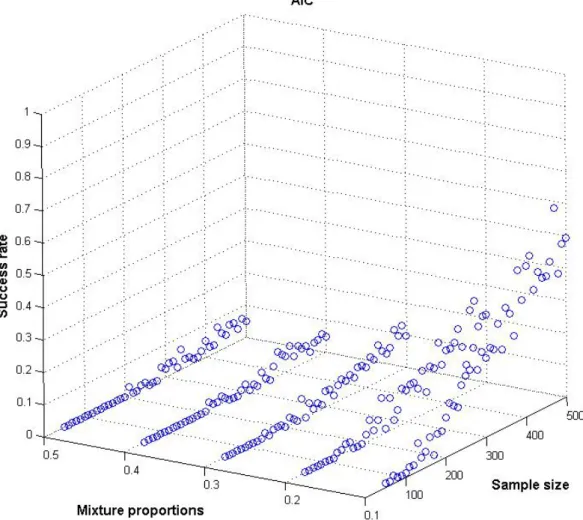
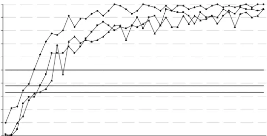
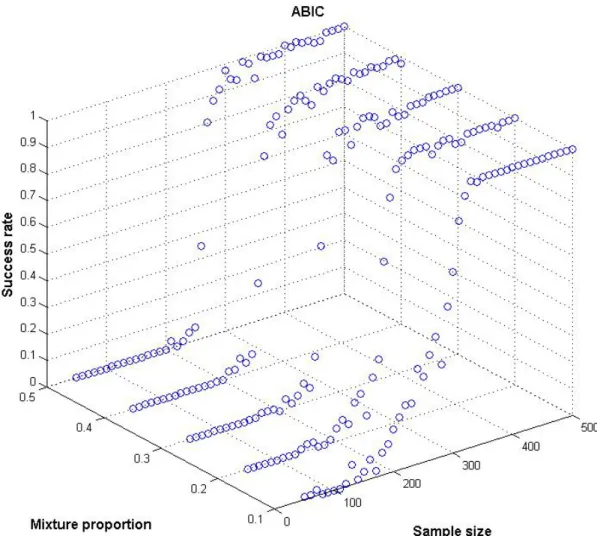
The following figures illustrate the findings of the simulation run. 3d-scatterplots are used to show the success rates for all sample/segment size combinations. Line charts demonstrate the distribution of success rates for ( 0.1, 1 0.9)

2 1 1 = π = π , ( 0.3, 3 0.7) 2 3 1 = π = π and ) 5 . 0 , 5 . 0 ( 5 2 5 1 = π =

π .Vertical dotted lines illustrate the boundaries of the previously mentioned chance models with Κ=

{

M1,M2,M3

}

: 0,33

3

1 _≈

=

ran

CM (lower dotted line), CM_prop =0,38

(15)

As can be seen in figures 1 and 2, the AIC only behaves favourably in recovering the true number of segments, under the condition of one of the two segments being rather small. As the distribution of segment size approaches a uniform distribution, success rates decrease gradually. With respect to absolute performance, the AIC produces adequate solutions for

when the random chance criterion is considered. 370

≥

n

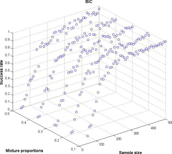
The performance of the BIC (figures 3 and 4) seems to be widely independent from the variation of the mixture proportions, showing slight advantageous performance in the presence of niche segments. As sample size increases, success rates grow up to the maximum of 100% for all mixture proportions. The criteria’s absolute performance is already favourable for sample sizes as low as n=100 against the background of the chance models.

(16)

AIC 0 0,1 0,2 0,3 0,4 0,5 0,6 0,7 0,8 0,9 1 50 100 150 200 250 300 350 400 450 500 Sample siz e S u cce ss r at e 0,1 0,3 0,5

Fig. 2: Comparison of AIC success rates for different sample/segment size combinations (2)

(17)

BIC 0 0,1 0,2 0,3 0,4 0,5 0,6 0,7 0,8 0,9 1 50 100 150 200 250 300 350 400 450 500 Sample siz e S u c cess r at e 0,1 0,3 0,5

Fig. 4: Comparison of BIC success rates for different sample/segment size combinations (2)

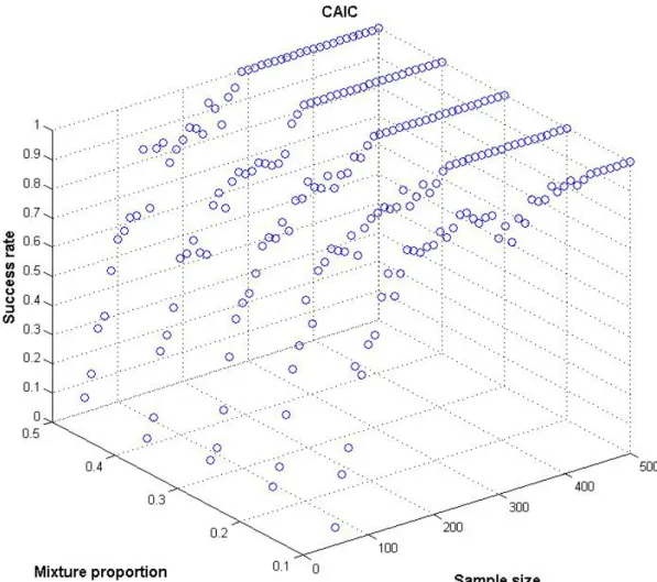
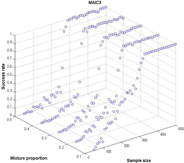
The following figures show that, regardless of mixture proportions, CAIC successfully identifies the correct number of segments and outperforms BIC in most cases. Independent from the existing mixture proportion, the maximum chance criterion is met for sample sizes as low as n = 100. Compared to BIC, the performance of CAIC is more consistent in terms of the development of the success rate across sample sizes. Despite its satisfying performance, the simulation results indicate that MAIC3 performs better in the presence of niche segments for sample sizes of n ≥ 290. In this range of sample sizes, ABIC3 and MAIC3 perform equally successful whereas the improvement in performance is more pronounced with MAIC3. Furthermore, it can be observed that for smaller sample sizes, only MAIC3 meets chance criterion standards if 1 0,1

1 =

π and 1 0,9 2 = π .

(18)

Fig. 5: Comparison of CAIC success rates for different sample/segment size combinations (1) CAIC 0 0,1 0,2 0,3 0,4 0,5 0,6 0,7 0,8 0,9 1 50 100 150 200 250 300 350 400 450 500 Sample siz e S u cce ss r a te 0,1 0,3 0,5

(19)

Fig. 7: Comparison of ABIC success rates for different sample/segment size combinations (1) ABIC 0 0,1 0,2 0,3 0,4 0,5 0,6 0,7 0,8 0,9 1 50 100 150 200 250 300 350 400 450 500 Sample siz e S u cc es s r at e 0,1 0,3 0,5

(20)

Fig. 9: Comparison of MAIC3 success rates for different sample/segment size combinations (1) MAIC3 0 0,1 0,2 0,3 0,4 0,5 0,6 0,7 0,8 0,9 1 50 100 150 200 250 300 350 400 450 500 Sample siz e S u cces s r at e 0,1 0,3 0,5

(21)

5. Key Contributions and Future Research Directions

The findings presented in this paper are relevant to a large number of researchers building models using mixture regression analysis. This study extends previous studies by evaluating how the interaction of sample and segment size affects the performance of five of the most widely used information criteria for assessing the true number of segments in mixture regression models. For the first time the quality of these criteria was evaluated for a wide spectrum of possible constellations. Furthermore relative and absolute performances against outside criteria were analyzed. The results induce recommendations on criterion selection when a certain sample size is given and help to judge what sample size is needed in order to guarantee an accurate decision based on a certain criterion respectively. The results also show that in the presence of certain sample/segment size combinations, decisions grounded on a specific criterion might prove problematic.

AIC demonstrates an extremely poor performance across all simulation situations. From an application-oriented point of view, this proves to be problematic, taking into account the high percentage of studies relying on this criterion to assess the number of segments in the model, making the appropriateness of these studies highly questionable. With regard to AIC, the results contrast the findings by OLIVEIRA-BROCHADO and MARTINS (2006) who certified this

criterion to perform well in a simulation design with equal segment sizes. In addition, AIC performs much worse in this study than in ANDREWS and CURRIM (2003b).

CAIC performs favourably, showing slight weaknesses in determining the true number of segments for high sample sizes in the presence of niche segments. In the latter situation, MAIC3 performs well, quickly achieving success rates of over 90%, hence meeting random chance, proportional chance and maximum chance boundaries. In contrast to previous findings by ANDREWS and CURRIM (2003b), CAIC outperforms BIC across all

sample/segment size combinations, whereupon the deviation is marginal when the segments of the mixture are not well separated ( 1 0,1

1 =

π and 2 0,2 1 =

π ). ABIC and MAIC3 all show a relative and absolute positive performance for high sample sizes, which haven’t yet been considered in previous studies.

Interestingly most criteria perform better in the presence of niche segments, which is an unexpected finding, since one might expect that the existence of a small segment adds complexity to the retention problem. Perhaps, this finding is attributed to the design of the

(22)

second (niche) segment with regard to the sizable mean separation between the regression coefficients of both segments.

The study at hand surely is not the final word on the advantageousness of model selection criteria in a mixture regression context. Further research is necessary assessing the interaction of sample or segment size and other factors such as number or measurement level of predictors on a larger scale. This topic should be addressed for other model types such as multinomial or zero-inflated regression models. The continued research on the performance of model selection criteria is needed in order to provide practical guidelines for disclosing the true number of segments in a mixture and to guarantee accurate conclusions for marketing practice.

However, considering the great number of research projects, one generally has to be critical with the idea of finding a unique measure that can be considered optimal in every simulation design or even practical applications, as indicated in other studies. Model selection decisions should rather be based on various evidences, not only derived from the data at hand but also from theoretical considerations. This requires additional elaborations of possibilities to include a-priori information or expected costs of under- or oversegmentation directly into the design of model selection criteria to merge data- and theory-driven assessment of marketing problems. The integration of a-priori information might enhance plausibility of the results and support the diffusion of this very promising technique in marketing practice.

(23)

Appendix

Year Author(s) Criterion/Criteria

2000 Bell/Lattin BIC

2000 Heilman et al. BIC

2000 Shachar/Emerson AIC, BIC, CAIC

2000 Mazumdar/Papatla BIC

2001 Thomas AIC

2001 Erdem et al. BIC

2001 Danaher/Mawhinney BIC

2001 Gönül et al. AIC, BIC

2002 Wedel/DeSarbo CAIC

2002a Andrews et al. BIC

2002a Hofstede et al. LMD

2002b Andrews et al. BIC, LMD

2002b Hofstede et al. LMD

2002 Danaher BIC

2002 Papatla/Bhatnagar BIC

2003 Agarwal BIC

2003 Danaher et al. BIC

2003 Ho/Chong n.s.

2003 Wu/Rangaswamy AIC, BIC, MAIC3

2003 Chung/Rao LMD

2004 Bowman et al. AIC, BIC

2004 Lewis BIC

2004 Anand/Shachar BIC

2004 Varki/Chintagunta BIC

2004 Zhang/Krishnamurthi BIC

2005 Reinartz et al. AIC

2005 Lewis BIC

2005 Thomas/Sullivan AIC

2005 Rust/Verhoef AIC, BIC, MAIC3

2005 Jedidi/Kohli BIC

2006 Srinivasan BIC

2006 Kivetz et al. BIC

2006 Mantrala et al. BIC

(24)

References

AGARWAL,M.K.(2003):Developing Global Segments and Forecasting Market Shares: A

Simultaneous Approach Using Survey Data, in: Journal of International Marketing, Vol. 11, p. 56-80.

AITKIN,M.;RUBIN,D.B.(1985): Estimation and Hypothesis Testing in Finite Mixture

Models, in: Journal of the Royal Statistical Society, Series B, Methodological, p. 67-75. AKAIKE,H. (1973): Information Theory and an Extension of the Maximum Likelihood

Principle, in: PETROV,B.N.;CSAKI,F. [Eds.]: Second International Symposium on

Information Theory, Budapest, p. 267-281.

ANAND,B.N.;SHACHAR,R.(2004):Brands as Beacons: A New Source of Loyalty to

Multiproduct Firms, in: Journal of Marketing Research, Vol. 41, p. 135-150.

ANDREWS,R.L.;AINSLIE,A.;CURRIM,I.S.(2002a):An Empirical Comparison of Logit

Choice Models with Discrete Versus Continuous Representations of Heterogeneity, in: Journal of Marketing Research, Vol. 39, p. 479-487.

ANDREWS,R.;ANSARI,A.;CURRIM,I. (2002b): Hierachical Bayes Versus Finite Mixture

Conjoint Analysis Models: A Comparison of Fit, Prediction and Pathworth Recovery, in: Journal of Marketing Research, Vol. 39, p. 87-98.

ANDREWS,R.;CURRIM,I. (2003a): A Comparison of Segment Retention Criteria for Finite

Mixture Logit Models, in: Journal of Marketing Research, Vol. 15, p. 235-243. ANDREWS,R.;CURRIM,I.(2003b): Retention of Latent Segments in Regression-based

Marketing Models, in: International Journal of Research in Marketing, Vol. 20, p. 315-321. BELL,D.R.;LATTIN,J.M. (2000): Looking for Loss Aversion in Scanner Panel Data: The

Confounding Effect of Price Response Heterogeneity, in: Marketing Science, Vol. 19, p. 185-200.

(25)

BIERNACKI,C.;CELEUX,G.;GOVAERT,G. (2000): Assessing a Mixture

Model for Clustering with the Integrated Completed Likelihood, in: IEEE Transactions on Pattern Analysis and Machine Intelligence, Vol. 22, p. 719-725.

BOWMAN,D.;HEILMAN,C.M.;SEETHARAMAN,P.B.(2004): Determinants of Product-Use

Compliance Behavior, in: Journal of Marketing Research, Vol. 41, p. 324-228. BOZDOGAN,H.;SCLOVE,S.L.(1984): Multi-sample Cluster Analysis using Akaike’s

Information Criterion, in: Annals of the Institute of Statistical Mathematics, Vol. 36, p. 163-180.

BOZDOGAN,H. (1987): Model Selection and Akaike’s Information Criterion (AIC): The

General Theory and its Analytical Extensions, in: Psychometrika, Vol. 52, p. 346-370. BOZDOGAN,H. (1990): On the Information-based Measure of Covariance Complexity and its

Application to the Evaluation of Multivariate Linear Models, in: Communications in Statistics, Theory and Methods, Vol. 19, No. 1, p. 221-278.

BOZDOGAN,H. (1993): Choosing the Number of Component Clusters in the Mixture-Model

using a New Information Complexity Criterion of the Inverse-Fisher Information Matrix, in: OPITZ,O.;KLAR,R. [Eds.]: Information and Classification, Heidelberg, p. 40-54.

BOZDOGAN,H. (1994): Mixture-model Cluster Analysis using Model Selection Criteria and a

new Information Measure of Complexity, in: Proceedings of the First US/Japan Conference on Frontiers of Statistical Modelling: An Informational Approach, Vol. 2, Boston, p. 69-113. BRAME,R.;NAGIN,D.S.;WASSERMAN,L.(2006): Exploring Some Analytical Characteristics

of Finite Mixture Models, in: Journal of Quantitative Criminology, Vol. 22, p. 31-59.

BUCKLIN,R.E.;GUPTA,S. (1992): Brand Choice, Purchase Incidence, and Segmentation: An

Integrated Modeling Approach, in: Journal of Marketing Research, Vol. 29, p. 201-215. CELEUX,G.;SOROMENHO,G. (1996): An Entropy Criterion for assessing the Number of

(26)

CHUNG,J.;RAO,V.R.(2003): A General Choice Model for Bundles with Multiple-Category

Products: Application to Market Segmentation and Optimal Pricing for Bundles, in: Journal of Marketing Research, Vol. 40, p. 115-130.

COX,D.R. (1972): Regression Models and Life-Tables, in: Journal of the Royal Statistical

Society. Series B (Methodological), Vol. 34, p. 187-220.

CUTLER,A.;WINDHAM,M.P. (1993): Information-based Validity Functionals for Mixture

Analysis, in: BOZDOGAN,H. [Ed.]: Proceedings of the first US-Japan Conference on Frontiers

of Statistical Modelling, Amsterdam, p. 149-170.

DANAHER,P.J.;MAWHINNEY D.F.(2001): Optimizing Television Program Schedules Using

Choice Modeling, in: Journal of Marketing Research, Vol. 38, p. 298-312.

DANAHER,P.J.(2002): Optimal Pricing of New Subscription Services: Analysis of a Market

Experiment, in: Marketing Science, Vol. 21, p. 119-138.

DANAHER,P.J.;WILSON,I.W.;DAVIS,R.A.(2003):A Comparison of Online and Offline

Consumer Brand Loyalty, in: Marketing Science, Vol. 22, p. 461-476.

DEMPSTER,A.P.;LAIRD,N.M;RUBIN,D.B.(1977): Maximum Likelihood from Incomplete

Data via the EM-Algorithm, in: Journal of the Royal Statistical Society, Series B, Vol. 39, p. 1-39.

DESEARBO,W.S.;DEGERATU,A.;WEDEL,M.;SAXTON,M. (2001a): The Spatial

Representation of Market Information, in: Marketing Science, Vol. 20, p. 426-441.

DESARBO,W.S.;JEDIDI,K.;SINHA,I. (2001b): Customer Value Analysis in a Heterogeneous

Market, in: Strategic Management Journal, Vol. 22, p. 845-857.

DILLON,W.R.;KUMAR,A. (1994): Latent Structure and Other Mixture Models in Marketing:

An Integrative Survey and Overview, in: BAGOZZI,R.P. [Ed.]: Advanced Methods of

(27)

ERDEM,T.;MAYHEW,G.;SUN,B. (2001): Understanding Reference-Price Shoppers: A

Within- and Cross-Category Analysis, in: Journal of marketing Research, Vol. 38, p. 445-457. EVERITT,B.S. (1981): A Monte Carlo Investigation of the Likelihood Ratio Test for the

Number of Components in a Mixture of Normal Distributions, in: Multivariate Behavioral Research, Vol. 16, p. 171-180.

EVERITT,B.S. (1988): A Monte Carlo Investigation of the Likelihood Ratio Test for Number

of Classes in Latent Class Analysis, in: Multivariate Behavioral Research, Vol. 23, p. 531-538.

GÖNÜL,F.F.;CARTER,F.;PETROVA,E.;SRINIVASAN,K.(2001): Promotion of Prescription

Drugs and Its Impact on Physicians` Choice Behavior, in: Journal of Marketing, Vol. 65, p. 79-90.

GRÜN,B.;LEISCH,F. (2006a): Fitting Finite Mixtures of Linear Regression Models with

Varying & Fixed Effects in R, in: RIZZI,A.;VICHI,M.[Eds.]: COMPSTAT 2006 –

Proceedings in Computational Statistics. 17th Symposium Held in Rome, Italy, 2006, Heidelberg.

GRÜN,B.;LEISCH,F.(2006b): Fitting Mixtures of Generalized Linear Regressions in R, in:

Computational Statistics and Data Analysis, 2006, in press.

HAHN,C.;JOHNSON,M.D.;HERRMANN,A.;HUBER,F.(2002): Capturing Customer

Heterogeneity using a Finite Mixture PLS Approach, in: Schmalenbach Business Review, Vol. 54, p. 243-269.

HARZING,A.(2006): Journal Quality List, 23rd edition, University of Melbourne, White Paper,

published electronically: [URL]: http://www.harzing.com/donload/jql.zip [November 20th 2006].

HAWKINS,D.S.;ALLEN,D.M.;STROMBERG,A.J. (2001): Determining the Number of

Components in Mixtures of Linear Models, in: Computational Statistics & Data Analysis, Vol. 38, p. 15-48.

(28)

HEILMAN,C.M.;BOWMAN,D.;WRIGHT,G.P.(2000): The Evoulution of Brand Perfernces

and Choice Behaviors of Consumers New to a Market, in: Journal of Marketing Research, Vol. 37, p. 139-155.

HO,T.;CHONG,J.(2003): A Parsimonious Model of Stockkeeping-Unit Choice, in: Journal of

Marketing Research, Vol. 40, p. 351-365.

HOFSTEDE,F.T.;KIM,Y.;WEDEL,M.(2002a): Bayesian Prediction in Hybrid Conjoint

Analysis, in: Journal of Marketing Research, Vol. 39, p. 253-261.

HOFSTEDE,F.T.;WEDEL,M.;STEENKAMP J.E.M. (2002b): Identifying Spatial Segments in

International Markets, in: Marketing Science, Vol. 21, p. 160-177.

ISHIGURO,M.;SAKAMOTO,Y.;KITAGAWA,G. (1997): Bootstrapping Log Likelihood and EIC.

An Extension of AIC, in: The Annals of the Institute of Statistical Mathematics, Vol. 49, No. 3, p. 411-434.

JEDIDI,K.;JAGPAL,H.S.;DESARBO,W.S.(1979): Finite-Mixture Structural Equation Models

for Response-Based Segmentation and Unobserved Heterogeneity, in: Marketing Science, Vol. 16, p. 39-59.

JEDIDI,K.;KOHLI,R. (2005): Probabilistic Subset-Conjunctive Models for Heterogeneous

Consumers, in: Journal of Marketing Research, Vol. 42, p. 483-494.

JEFFRIES,N.O.(2003): A Note on “Testing the Number of Components in a Normal

Mixture”, in: Biometrika, Vol. 90, p. 991-994.

KIVETZ,R.;URMINSKY,O.;ZHENG,Y.(2006): The Goal-Gradient Hypothesis Resurrected:

Purchase Acceleration, Illusionary Goal Progress, and Customer Retention, in: Journal of Marketing Research, Vol. 43, p. 39-58.

KOEHLER,A.B.;MURPHREE,E.H. (1988): A Comparison of the Akaike and Schwarz Criteria

(29)

LEISCH,F. (2004): FlexMix: A General Framework for Finite Mixture Models and Latent

Class Regresion in R, in: Journal of Statistical Software, Vol. 11, p. 1-18.

LEROUX, B. (1992): Consistent Estimation of a Mixing Distribution, in: Annals of

Statistics, Vol. 20, No. 3, p.1350-1360.

LEWIS,M.(2004): The Influence of Loyalty Programs and Short-Term Promotions on

Customer Retention, in: Journal of Marketing Research, Vol. 41, p. 281-292.

LEWIS,M.(2005): Incorporating Strategic Consumer Behavior into Customer Valuation, in:

Journal of Marketing, Vol. 69, p. 230-238.

LO,Y.;MENDELL,N.R.;RUBIN,D.B.(2001): Testing the Number of Components in a

Normal Mixture, in: Biometrika, Vol. 88, p. 767-778.

MANTRALA,M.K.; SEETHARAMAN,P. B.;KAUL,R.; GOPALAKRISHNA,S.; STAM,A.

(2006): Optimal Pricing Strategies for an Automotive Aftermarket Retailer, in: Journal of Marketing Research, Vol. 43, p. 588-604.

MAZUMDAR,T.;PAPATLA,P.(2000): An Investigation of Reference Prices Segments,

in: Journal of Marketing Research, Vol. 37, p. 246-258.

MCLACHLAN,G.J. (1987): On Bootstrapping the Likelihood Ratio Test Statistic for

the Number of Components in a Normal Mixture, in: Applied Statistics, Vol. 36, p. 318-324.

MCLACHLAN,G.J.;NG,S.K. (2000): A Comparison of some Information Criteria for

the Number of Components in a Mixture Model, Technical Report, Brisbane Department of Mathematics, University of Queensland.

MCLACHLAN, G. J.; PEEL, D. (2000): Finite Mixture Models, Wiley Series in

(30)

MORRISON,D.G.(1969): On the Interpretation of Discriminant Analysis, in: Journal of

Marketing Research, Vol. 6, p. 156-63.

MUTHÉN,L.K.;MUTHÉN,B.O.(2006): Mplus. Statistical Analysis with Latent Variables,

User’s Guide Version 4, Los Angeles, 2006.

NYLUND,K.L.;ASPAROUHOV,T.;MUTHÉN,B.O. (2006): Deciding on the Number of Classes

in Latent Class Analysis and Growth Mixture Modeling: A Monte Carlo Simulation Study, White Paper, published electronically: [URL]:

http://www.statmodel.com/download/LCA_tech11_nylund_v83.pdf [November 20th 2006]. OLIVEIRA-BROCHADO,A.;MARTINS,F.V.(2005):Assessing the Number of Components in

Mixture Models: A Review, FEP Working Papers, No. 194, published electronically: [URL]: http://www.fep.up.pt/investigacao/workingpapers/05.11.03_WP194_brochadovitorino.pdf [November 20th_2006]

OLIVEIRA-BROCHADO,A.;MARTINS,F.V.(2006): Examining the Segment Retention Problem

for the “Group Satellite” Case, FEP Working Papers, No. 220, published electronically: [URL]:

http://www.fep.up.pt/investigacao/workingpapers/06.07.04_WP220_brochadomartins.pdf [November 20th 2006].

PAPATLA,P.;BHATNAGAR,A.(2002): Shopping Style Segmentation of Consumer, in:

Marketing Letters, Vol. 13, p. 91-106.

RDEVELOPMENT CORE TEAM (2006): R. A Language and Environment for Statistical

Computing. R Foundation for Statistical Computing, Vienna: [URL]: http://www.R-project.org [November 20th 2006].

REINARTZ,W.;THOMAS,J.S.;KUMAR,V.(2005): Balancing Acquisition and Retention

Resources to Maximize Customer Profitability, in: Journal of Marketing, Vol. 69, p. 63-79. RISSANEN,J. (1978): Modelling by Shortest Data Description, in: Automatica, Vol. 14, p.

(31)

RODRÍGUEZ,C.C.(2005): The ABC of Model Selection: AIC, BIC and the New CIC, White

Paper, Department of Mathematics and Statistics, The University of Albany, SUNY, published electronically: [URL]: http://omega.albany.edu:8008/CIC/me05.pdf [November 20th 2006].

RUST,R.T.;SIMESTER,D.;BRODIE,R.J.;NILIKANT,V. (1995): Model Selection Criteria: An

Investigation of Relative Accuracy, Posterior Probabilities and Combinations of Criteria, in: Management Science, Vol. 41, No. 2, p. 322-333.

RUST,R.T.;VERHOEF,P.C.(2005):Optimizing the Marketing Interventions Mix in

Intermediate-Term CRM, in: Marketing Science, Vol. 24, p. 477-489.

SCHWARZ,G.(1978): Estimating the Dimensions of a Model, in: The Annals of Statistics,

Vol. 6, p. 461-464.

SCLOVE,S.L. (1987): Application of Model-Selection Criteria to Some Problems in

Multivariate Analysis, in: Psychometrika, Vol. 52, p. 333-343.

SHACHAR,R.;EMERSON,J.W.(2000): Cast Demographics, Unobserved Segments, and

Heterogeneous Switching Costs in an Television Viewing Choice Model, in: Journal of Marketing Research, Vol. 37, p. 173-186.

SJOQUIST, D. L.; WALKER, M. B.; WALLACE, S. (2003): Estimating Differential

Responses to Local Fiscal Conditions: A Mixture Model Analysis, Working Paper, Department of Economics, Andrew Young School of Policy Studies, Georgia State University, published electronically: [URL]:

http://frp.aysps.gsu.edu/sjoquist/works/Mixture%20Paper%207-02-03.pdf [November 20th 2006].

SOROMENHO,G.(1993): Comparing Approaches for Testing the Number of Components in a

Finite Mixture Model, in: Computational Statistics, Vol. 9, p. 65-78.

SRINIVASAN,R. (2006): Dual Distribution and Intangible Firm Value: Franchising in

(32)

THOMAS,J.S.(2001): A Methodology for Linking Customer Acquisition to Customer

Retention, in: Journal of Marketing Research, Vol. 38, p. 262-268.

THOMAS,J.S.;SULLIVAN,U.Y.(2005): Managing Marketing Communications with

Multichannel Customers, in: Journal of Marketing, Vol. 69, p. 239-251.

TITTERINGTON,D.M.;SMITH,A.F.M.;MAKOV,U.E.(1985): Statistical Analysis of Finite

Mixture Distributions, New York, 1985.

TOFIGHI,D.;ENDERS,C.K.(2007): Identifying the Correct Number of Classes in Growth

Mixture Models, in: HANCOCK,G.R.;SAMUELSON,K.M.[Eds.]: Advances in Latent Variable

Mixture Models, Greenwhich, in press.

VARKI,S.;CHINTAGUNTA,P.K,(2004): The Augmented Latent Class Model: Incorporating

Additional Heterogeneity in the Latent Class Model for Panel Data, in: Journal of Marketing Research, Vol. 41, p. 226-233.

VERMUNT,J.K.;MAGIDSON,J. (2005): Latent Gold 4.0 – User’s Guide, published

electronically: [URL]: http://www.statisticalinnovations.com/products/fullmanual.pdf [November 20th 2006].

WEDEL,M.;KAMAKURA,W.A. (1999): Market Segmentation. Conceptual and

Methodological Foundations, Boston et al., 1999.

WEDEL,M.;DESARBO,W.S. (2002): Market Segment Derivation and Profiling Via a Finite

Mixture Model Framework, in: Marketing Letters, Vol. 13, p.17-25.

WOODROOFE,M. (1982): On Model Selection and the Arc Sine Law, in: Annals of Statistics,

Vol. 10, p. 1182-1194.

WU,J.;RANGASWAMY,A.(2003): A Fuzzy Set Model of Search and Consideration with an

(33)

YANG,C.(2006): Evaluating Latent Class Analysis in Qualitative Phenotype Identification,

in: Computational Statistics & Data Analysis, Vol. 50, p. 1090-1104.

YOO,S.(2003): Application of a Mixture Model to Approximate Bottled Water Consumption

Distribution, in: Applied Economics Letters, Vol. 10, p. 181-184.

ZHANG,J.;KRISHNAMURTHI,L. (2004): Customizing Promotions in Online Stores, in:

Sample- and segment-size specific Model Selection in Mixture Regression Analysis