Assessing Fit of Item Response Models for Performance Assessments using Bayesian Analysis

ASSESSING FIT OF ITEM RESPONSE MODELS FOR PERFORMANCE ASSESSMENTS USING BAYESIAN ANALYSIS

by

Xiaowen Zhu

B.S., Southwest University of Science and Technology, 1996

Submitted to the Graduate Faculty of School of Education in partial fulfillment

of the requirements for the degree of Doctor of Philosophy

University of Pittsburgh 2009

UNIVERSITY OF PITTSBURGH SCHOOL OF EDUCATION

This dissertation was presented

by

Xiaowen Zhu

It was defended on November 20, 2009

and approved by

Clement A. Stone, Professor, Psychology in Education Suzanne Lane, Professor, Psychology in Education Feifei Ye, Assistant Professor, Psychology in Education

James E. Bost, Associate Professor, Center for Research on Health Care Dissertation Advisor: Clement A. Stone, Professor, Psychology in Education

Copyright © by Xiaowen Zhu 2009

Assessing IRT model-fit and comparing different IRT models from a Bayesian perspective is gaining attention. This research evaluated the performance of Bayesian model-fit and model-comparison techniques in assessing the fit of unidimensional Graded Response (GR) models and comparing different GR models for performance assessment applications.

The study explored the general performance of the PPMC method and a variety of discrepancy measures (test-level, item-level, and pair-wise measures) in evaluating different aspects of fit for unidimensional GR models. Previous findings that the PPMC method is conservative were confirmed. In addition, PPMC was found to have adequate power in detecting different aspects of misfit when using appropriate discrepancy measures. Pair-wise measures were found more powerful in detecting violations of unidimensionality and local independence assumptions than test-level and item-level measures. Yen’s Q3measure appeared to perform best. In addition, the power of PPMC increased as the degree of multidimensionality or local dependence among item responses increased. Two classical item-fit statistics were found effective for detecting the item misfit due to discrepancies from GR model boundary curves.

The study also compared the relative effectiveness of three Bayesian model-comparison indices (DIC, CPO, and PPMC) for model selection. The results showed that these indices appeared to perform equally well in selecting a preferred model for an overall test. However, the advantage of PPMC applications is that they can be used to compare the relative fit of different

ASSESSING FIT OF ITEM RESPONSE MODELS FOR PERFORMANCE ASSESSMENTS USING BAYESIAN ANALYSIS

Xiaowen Zhu, PhD University of Pittsburgh, 2009

models, but also evaluate the absolute fit of each individual model. In contrast, the DIC and CPO indices only compare the relative fit of different models.

This study further applied the Bayesian model-fit and model-comparison methods to three real datasets from the QCAI performance assessment. The results indicated that these datasets were essentially unidimensional and exhibited local independence among items. A 2P GR model provided better fit than a 1P GR model, and a two-dimensional model was also not preferred. These findings were consistent with previous studies, although Stone’s fit statistics in the PPMC context identified less misfitting items compared to previous studies. Limitations and future research for Bayesian applications to IRT are discussed.

TABLE OF CONTENTS

PREFACE ... XIX

1.0 INTRODUCTION ... 1

1.1 STATEMENT OF THE PROBLEM ... 1

1.2 SIGNIFICANCE OF THE STUDY ... 6

1.3 LIMITATIONS OF THE STUDY ... 8

2.0 REVIEW OF LITERATURE ... 9

2.1 APPLICATIONS OF IRT TO PERFORMANCE ASSESSMENTS ... 9

2.1.1 Brief Introduction to Performance Assessments ... 9

2.1.2 IRT Models for Performance Assessments ... 11

2.1.2.1 General Description ... 11

2.1.2.2 Graded Response Model (Samejima, 1969) ... 13

2.1.3 Main Threats in Applying Unidimensional IRT Models to PAs ... 17

2.1.3.1 Multidimensionality ... 17

2.1.3.2 Local Dependence ... 20

2.2 TRADITIONAL METHODS FOR CHECKING IRT MODEL-FIT ... 23

2.2.1 Assessing Dimensionality ... 23

2.2.2 Detecting Local Dependence ... 25

2.2.3.1 Traditional Item-Fit Statistics ... 28

2.2.3.2 Alternative Item-Fit Statistics ... 30

2.3 POSTERIOR PREDICTIVE MODEL CHECKING (PPMC) IN A BAYESIAN FRAMEWORK ... 33

2.3.1 Introduction to Bayesian Inference... 33

2.3.2 Posterior Predictive Model Checking (PPMC) ... 35

2.3.2.1 Description of PPMC Method ... 35

2.3.2.2 Computation via MCMC Simulation ... 38

2.3.2.3 Discrepancy Measures ... 39

2.3.2.4 Advantages of PPMC over Classical Model-Fit Tests ... 41

2.3.3 Markov Chain Monte Carlo (MCMC) Simulation ... 41

2.3.3.1 Definition... 41

2.3.3.2 Convergence Diagnosis ... 44

2.4 CHECKING IRT MODEL-FIT USING PPMC ... 47

2.4.1 Advantages of Using PPMC in IRT ... 47

2.4.2 Discrepancy Measures Used with Dichotomous IRT Models ... 49

2.4.2.1 Test-Level Discrepancy Measures ... 49

2.4.2.2 Item-Level Discrepancy Measures ... 51

2.4.2.3 Pair-wise Discrepancy Measures ... 53

2.4.3 Previous Research... 58

2.5 MODEL COMPARISON IN A BAYESIAN FRAMEWORK ... 62

2.5.1 Pseudo-Bayes Factor (PsBF)... 63

3.0 METHODOLOGY ... 68

3.1 SIMULATION STUDY 1... 69

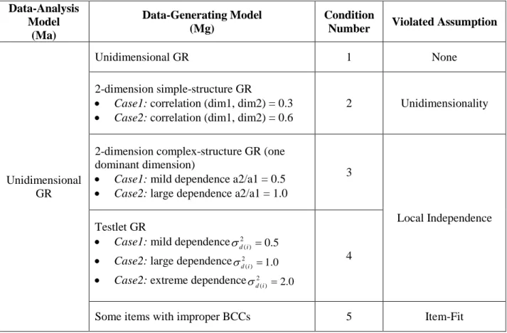
3.1.1 Design of Simulation Study 1 ... 69

3.1.2 Generate and Validate Item Response Data ... 75

3.1.3 Estimate Unidimensional GR Model in WinBUGS ... 91

3.1.4 Discrepancy Measures Used in Study 1 ... 96

3.1.5 Conduct PPMC ... 103

3.2 SIMULATION STUDY 2... 107

3.2.1 Design of Simulation Study 2 ... 107

3.2.2 Generate Item Response Data ... 109

3.2.3 Estimate Different Data-Analysis Models in WinBUGS... 110

3.2.4 Conduct Model Comparison... 126

3.3 REAL DATA APPLICATION ... 130

4.0 RESULTS ... 136

4.1 RESULTS FROM SIMULATION STUDY 1 ... 136

4.1.1 Item Parameter Recovery ... 137

4.1.2 Condition 1 (Ma = Mg = unidimensional GR) ... 138

4.1.3 Condition 2 (Mg = 2-dim simple-structure GR , Ma = 1-dim GR) ... 149

4.1.4 Condition 3 (Mg = 2-dim complex-structure GR , Ma = 1-dim GR) ... 158

4.1.5 Condition 4 (Mg = testlet GR , Ma = 1-dim GR) ... 167

4.1.6 Condition 5 (Mg = items with improper BCCs , Ma = 1-dim GR) ... 177

4.2 RESULTS FROM SIMULATION STUDY 2 ... 182

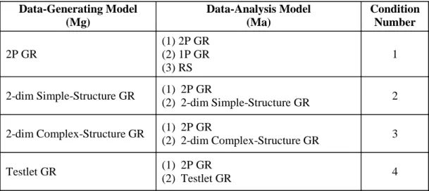
4.2.2 Condition 2 (1-dim GR vs. 2-dim simple-structure GR model) ... 193

4.2.3 Condition 3 (1-dim GR vs. 2-dim complex-structure GR model) ... 199

4.2.4 Condition 4 (1-dim GR model vs. GR model for testlet) ... 206

4.3 RESULTS FROM REAL APPLICATION ... 212

4.3.1 QCAI Data 1 – AS91 ... 212

4.3.2 QCAI Data 2 – AS92 ... 222

4.3.3 QCAI Data 3 – BS92 ... 228

5.0 DISCUSSION ... 236

5.1 SUMMARY OF MAJOR FINDINGS ... 236

5.1.1 Simulation Study 1... 236

5.1.2 Simulation Study 2... 244

5.1.3 Real Application ... 246

5.2 LIMITATIONS AND FUTURE RESEARCH DIRECTIONS ... 248

APPENDIX A ... 251 APPENDIX B ... 254 APPENDIX C ... 255 APPENDIX D ... 259 APPENDIX E ... 261 APPENDIX F ... 263 BIBLIOGRAPHY ... 276

LIST OF TABLES

Table 3.1 Design and Conditions in Study 1 ... 69

Table 3.2 Item Parameters of the IRT Models under Conditions 1-5 ... 76

Table 3.3 Absolute Differences between Observed and Expected Proportions under GR Model 78 Table 3.4 Item Parameter Recovery under Unidimensional GR Model ... 79

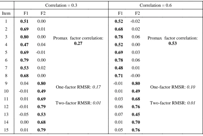
Table 3.5 Factor Analyses of Generated 2-dimensional Simple-Structure Data ... 82

Table 3.6 Local Dependence Test (p-values of Chi-Square Statistics) in IRTFIT – Case 2 ... 85

Table 3.7 Local Dependence Tests (Residual Correlations) in IRTFIT - Case 2 ... 86

Table 3.8 Average Absolute Residual Correlations for Different Levels of Dependency ... 87

Table 3.9 Average Absolute Residual Correlations for Different Testlet Effects ... 89

Table 3.10 Expected and Observed Proportions for Two Misfitting Items ... 91

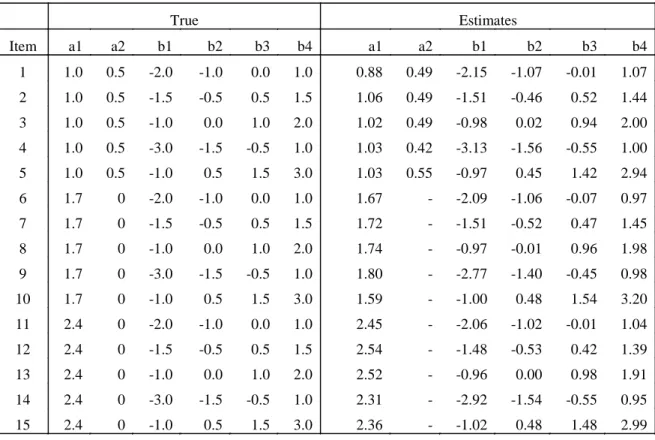
Table 3.11 Item Parameter Recovery using MCMC Estimation for the GR Model... 96

Table 3.12 Design and Conditions in Simulation Study 2 ... 108

Table 3.13 Item Parameter Recovery for 1P GR Model in WinBUGS ... 113

Table 3.14 Item Parameter Recovery for RS Model in WinBUGS ... 116

Table 3.15 Item Parameter Recovery for 2-dim Simple-Structure GR Model in WinBUGS .... 119

Table 3.16 Item Parameter Recovery for 2-dim Complex-Structure GR Model in WinBUGS . 123 Table 3.17 Item Parameter Recovery for Testlet GR Model in WinBUGS ... 126

Table 3.18 Misfitting Items Identified in Stone et al. (1993) and Stone (2000) ... 135

Table 4.1 RMSD for Item Parameter Recovery in WinBUGS for GR Model ... 137

Table 4.2 Median PPP-values and Average Proportions of Replications with Extreme PPP-values (< 0.05 or >0.95) when Ma=Mg=unidimensional GR ... 139

Table 4.3 Median PPP-values and Proportions of Replications with Extreme PPP-values for Item-Level Meausres when Ma=Mg=unidimensional GR ... 143

Table 4.4 Overall Median PPP-values and Average Proportions of Replications with Extreme PPP-values for all Measures – Condition 2 ... 149

Table 4.5 Overall Median PPP-values and Average Proportion of 20 Replications with Extreme PPP-values for all Measures – Condition 3 ... 158

Table 4.6 Overall Median PPP-values and Average Proportion of 20 Replications with Extreme PPP-values for all Measures – Condition 4 ... 167

Table 4.7 Overall Median PPP-values and Average Proportion of Replications with Extreme PPP-values for all Measures – Condition 5 ... 177

Table 4.8 RMSD for Item Parameter Recovery in WinBUGS for 2P GR Model ... 183

Table 4.9 Model Selection for Overall Test using DIC and Test-Level CPO – Condition 1 ... 184

Table 4.10 Model Selection for Each Item using Item-Level CPO Index – Condition 1 ... 185

Table 4.11 Number of Items with Extreme PPP-values across 20 Replications (Item-level Measures) ... 187

Table 4.12 Number of Item-pairs with Extreme PPP-values across 20 Replications (Pair-wise Measures) ... 188

Table 4.14 RMSD for Item Parameter Recovery in WinBUGS for 2-dim Simple-Structure

Model ... 193

Table 4.15 Model Selection for Overall Test using Different Indices – Condition 2 ... 194

Table 4.16 Model Selection for Each Item using Item-level CPO Index – Condition 2 ... 197

Table 4.17 RMSD for Item Parameter Recovery in WinBUGS for 2-dim Complex-Structure Model ... 199

Table 4.18 Model Selection for Overall Test using Different Indices – Condition 3 ... 200

Table 4.19 Model Selection of Each Item using Item-level CPO Index – Condition 3 ... 202

Table 4.20 RMSD for Item Parameter Recovery in WinBUGS for Testlet GR Model ... 206

Table 4.21 Model Selection for Overall Test using Different Indices – Condition 4 ... 207

Table 4.22 Model Selection for Each Item using Item-level CPO Index – Condition 4 ... 209

Table 4.23 Item Parameter Estimates using WinBUGS and Multilog – AS91 ... 213

Table 4.24 PPP-values for Item-level Measures based on GR and 1P GR Models – AS91 ... 214

Table 4.25 Model Selection Indices for Overall Test – AS91 ... 220

Table 4.26 Item-level CPO Index for Each Item – AS91 ... 220

Table 4.27 Item Parameter Estimates using WinBUGS and Multilog – AS92 ... 222

Table 4.28 PPP-values for Item-level Measures based on GR and 1P GR Models – AS92 ... 224

Table 4.29 Model Selection Indices for Overall Test – AS92 ... 227

Table 4.30 Item Parameter Estimates using WinBUGS and Multilog – BS92 ... 228

Table 4.31 PPP-values for Item-level Measures based on GR and 1P GR Models – BS92 ... 229

LIST OF FIGURES

Figure 2.1 Boundary Category Curves for a 5-category Item under the GR Model ... 15

Figure 2.2 Category Response Curves for a 5-category Item under the GR Model ... 16

Figure 2.3 Examples of Graphical Displays in PPMC by using Histograms ... 37

Figure 2.4 Examples of Graphical Displays in PPMC by using Scatter Plots ... 38

Figure 2.5 Graphical Description of Implementing the PPMC Method ... 39

Figure 2.6 History Plots Displaying Evidence of Convergence and Non-Convergence ... 44

Figure 2.7 Example of Observed and Predictive Test Score Distributions ... 50

Figure 3.1 Overall Steps in Conducting Simulation Study 1 ... 74

Figure 3.2 Boundary Category Curves (BCCs) for Two Misfitting Items ... 90

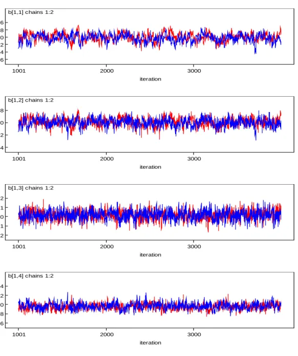
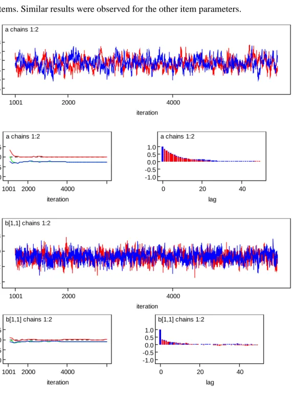
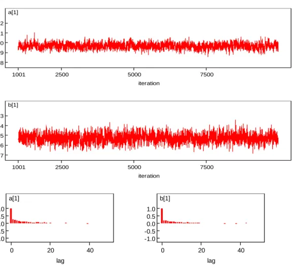
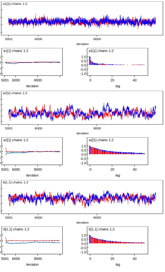
Figure 3.3 Sampling History Plots of Item Parameters Associated with Two Chains - Item 1 .... 93

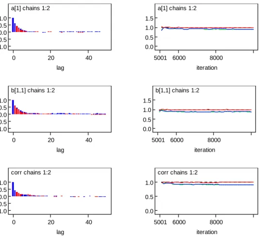
Figure 3.4 "BGR" Diagrams for the Parameters of Item 1 ... 94

Figure 3.5 Autocorrelation Plots for the Parameters of Item 1 ... 95

Figure 3.6 Example Convergence Diagnostic Plots for Item Parameters under 1P GR Model . 112 Figure 3.7 Example Convergence Diagnostic Plots for Item Parameters under RS Model ... 115

Figure 3.8 Convergence Diagnostic Plots for Parameters under 2-dim Simple-Structure GR Model ... 118

Figure 3.9 Convergence Diagnostic Plots for Parameters under 2-dim Complex-Structure GR Model ... 122 Figure 3.10 Convergence Diagnostic Plots for Parameters under Testlet GR Model ... 125 Figure 4.1 Distributions of PPP-values for Each Discrepancy Measures under the Null Condition ... 140 Figure 4.2 Diagnostic Plots based on Test Score Distribution when Ma=Mg=unidimensional GR ... 142 Figure 4.3 Oberved vs. 90% Posterior Preditive Interval of Item-Total Correlation for Each Item when Ma=Mg=undimensional GR ... 144 Figure 4.4 Realized vs. Posterior Predictive Values of Item-Level Chi-Square Measure and Yen’s Q1 for Item 1 when Ma=Mg=unidimensional GR ... 144

Figure 4.5 Display of Median PPP-values (Left) and Proportion of 20 Replications with Extreme PPP-values (Right) for Global OR (Row1), Yen’s Q3 (Row2), and Item Covariance Residual (Row3) when Ma=Mg= unidimensional GR ... 146 Figure 4.6 Display of PPP-values (based on a single dataset) for Yen’s Q3 (Left), and Item Covariance Residual (Right) when Ma=Mg= unidimensional GR ... 147 Figure 4.7 Observed vs. 90% Posterior Predictive Interval of Global OR for Item 1 with Other Items (for a single replication) when Ma=Mg= unidimensional GR ... 148 Figure 4.8 Scatter plots of Realized vs. Posterior Predictive Values of Yen’s Q3 and Item Covariance Residual (for a single data) when Ma=Mg= unidimensional GR ... 148 Figure 4.9 Display of Median PPP-values (Left) and Proportion of 20 Replications with Extreme PPP-values (Right) for Global OR (Row1), Yen’s Q3 (Row2), and Item Covariance Residual (Row3) – Condition 2 (ρ=0.6) ... 152

Figure 4.10 Display of PPP-values (based on a single dataset) for Yen’s Q3 (Left), and Item Covariance Residual (Right) - Condition 2 (ρ=0.6) ... 153 Figure 4.11 Scatter plots of Realized vs. Posterior Predictive Values of Yen’s Q3 (top), and Item Covariance Residual (bottom) (for a single data) – Condition 2 / Case 2 (ρ=0.6) ... 154 Figure 4.12 Observed vs. 90% Posterior Predictive Interval of Global OR for Item 1 with Other Items (for a single replication) – Condition 2 / Case 2 (ρ=0.6) ... 155 Figure 4.13 Observed vs. 90% Posterior Predictive Interval of Item-Total Score Correlation (Left) and Histogram of Predicted SDs (for a single replication) for Case 1 (top) and Case 2 (bottom) – Condition 2... 156 Figure 4.14 Diagnostic Plots based on Test Score Distribution (for a single data) – Condition2 /Case 1 ... 157 Figure 4.15 Scatter plots of Realized vs. Posterior Predictive Values of Yen’s Q3 (for a single data) for Case 1 (top) and Case 2 (bottom) – Condition 3 ... 161 Figure 4.16 Scatter plots of Realized vs. Posterior Predictive Values of Item Covariance Residual (for a single data) for Case 1 (top) and Case 2 (bottom) – Condition 3 ... 162 Figure 4.17 Observed vs. 90% Posterior Predictive Interval of Global OR for Item 1 with Other Items (for a single replication) for Case 1 (top) and Case 2 (bottom) – Condition 3 ... 163 Figure 4.18 Display of Median PPP-values (Left) and Proportion of 20 Replications with Extreme PPP-values (Right) for Global OR (Row1), Yen’s Q3 (Row2), and Item Covariance Residual (Row3) – Condition 3/ Case 1 ... 165 Figure 4.19 Display of Median PPP-values (Left) and Proportion of 20 Replications with Extreme PPP-values (Right) for Global OR (Row1), Yen’s Q3 (Row2), and Item Covariance Residual (Row3) – Condition 3/ Case 2 ... 166

Figure 4.20 Scatter Plots of Realized vs. Posterior Predictive Values of Yen’s Q3 (for a single data) for Case 1 (top) and Case 3 (bottom) – Condition 4 ... 169 Figure 4.21 Scatter Plots of Realized vs. Posterior Predictive Values of Item Covariance Residual (for a single data) for Case 1 (top) and Case 3 (bottom) – Condition 4 ... 169 Figure 4.22 Observed vs. 90% Posterior Predictive Interval of Global OR for Item 6 with Other Items (for a single replication) for Case 1 (top) and Case 3 (bottom) – Condition 4 ... 171 Figure 4.23 Display of Median PPP-values (Left) and Proportion of 20 Replications with Extreme PPP-values (Right) for Global OR (Row1), Yen’s Q3 (Row2), and Item Covariance Residual (Row3) – Condition 4/Case 1 ... 172 Figure 4.24 Display of Median PPP-values (Left) and Proportion of 20 Replications with Extreme PPP-values (Right) for Global OR (Row1), Yen’s Q3 (Row2), and Item Covariance Residual (Row3) – Condition 4/Case 3 ... 173 Figure 4.25 Observed vs. 90% Posterior Predictive Interval of Item-Total Score Correlation for Case 1 (top), Case 2 (middle), and Case 3 (bottom) based on a single replication – Condition 4 ... 176 Figure 4.26 Scatter plots of Realized vs. Posterior Predictive Values of Yen’s Q1 and Stone’s X2 Item-Fit Statistics (for a single data) – Condition 5 ... 180 Figure 4.27 Display of Median PPP-values (left) and Proportion of 20 Replications with Extreme PPP-values (right) for Global OR (row1), Yen’s Q3 (row2), and Item Covariance Residual (row3) – Condition 5 ... 181 Figure 4.28 Box-plots of DIC and Test-Level CPO across 20 Replications – Condition 1 ... 184 Figure 4.29 Observed vs. 90% Posterior Predictive Interval of Item-Total Score Correlation for 2P GR (top), 1P GR (middle), and RS (bottom) Model ... 191

Figure 4.30 Display of Median PPP-values for Pair-wise Measures when fitting 2P GR (top), 1P GR (middle), and RS(bottom) models to the Data ... 192 Figure 4.31 Box-plots of Model Comparison Indices across 20 Replications – Condition 2 ... 195 Figure 4.32 Display of Median PPP-values for Yen’s Q3 (left) and Global OR (right) when Fitting 1-dim GR model (top) and 2-dim simple-structure GR model (bottom) to the Data... 198 Figure 4.33 Box-plots of Model Comparison Indices across 20 Replications – Condition 3 ... 201 Figure 4.34 Display of Median PPP-values for Yen’s Q3 (left) and Global OR (right) when Fitting 1-dim GR Model (top) and 2-dim complex-structure GR Model (bottom) to the Data.. 204 Figure 4.35 Box-plots of Model Comparison Indices across 20 Replications – Condition 4 ... 208 Figure 4.36 Display of Median PPP-values for Yen’s Q3 (left) and Global OR (right) when fitting 1-dim GR Model (top) and testlet GR Model (bottom) to the Data ... 211 Figure 4.37 Example History and Autocorrelation Plots – AS91 ... 213 Figure 4.38 Observed vs. Expected ICCs for Misfitting Items on the AS91 Form ... 217 Figure 4.39 Display of PPP-values for Pair-wise Measures when fitting GR Model (top) and 1P GR Model (bottom) to the data – AS91 ... 219 Figure 4.40 Example History and Autocorrelation Plots – AS92 ... 223 Figure 4.41 Observed vs. Expected ICCs for Misfitting Items on the AS92 Form ... 225 Figure 4.42 Display of PPP-values for Pair-wise Measures when fitting GR Model (top) and 1P GR Model (bottom) to the Data – AS92 ... 226 Figure 4.43 Example History and Autocorrelation Plots – BS92 ... 228 Figure 4.44 Observed vs. Expected ICCs for Misfitting Items on the BS92 Form ... 232 Figure 4.45 Display of PPP-values for Pair-wise Measure when fitting GR Model (top) and 1P GR Model (bottom) to the Data – BS92 ... 233

ABBREVIATION TABLES 1P GR – one-parameter Graded Response

2P GR – two-parameter Graded Response

2-dim – two-dimensional

AIC – Akaike’s Information Criterion

AP – Advanced Placement

BCC – Boundary Category Curve

BIC – Bayesian Information Criterion

CPO – Conditional Predictive Ordinate

CTT – Classical Test Theory

DF – Degrees of Freedom

DIC – Deviance Information Criterion

DIF – Differential Item Functioning

GPC – Generalized Partial Credit

GR – Graded Response

ICC – Item Category Curves

IRT – Item Response Theory

LD – Local Dependence

LI – Local Independence

MC – Multiple-Choice

MCMC – Markov Chain Monte Carlo

M-H – Metropolis-Hastings

MH – Mantel Hanzel

MIRT – Multidimensional IRT

ML – Maximum Likelihood

MME – Marginal Maximum Likelihood

NAEP – National Assessment of Educational Progress

NR – Nominal Response

OCC – Operating Characteristic Curve

OR –Odds Ratio

PA – Performance Assessment

PC – Partial Credit

PPMC – Posterior Predictive Model Checking

PPP-value – Posterior Predictive P-value

PsBF – Pseudo-Bayes Factor

RS – Rating Scale

PREFACE

The following dissertation, while an individual work, benefited from the insights and direction of several people. First, I would like to express my deepest gratitude to Dr. Clement A. Stone, my advisor, for his guidance, caring, and tremendous support throughout my doctoral study. It is he who led me into the IRT model-fit area, sparked my interest in Bayesian methodologies, and introduced this interesting research topic to me. In addition, Dr. Stone provided timely and instructive comments and evaluation at every stage of my dissertation process. I truly appreciate his patient revision of my proposal and this dissertation.

Next, I would like to thank three other members in my dissertation committee, Dr. Suzanne Lane, Dr. Feifei Ye, and Dr. James E. Bost. Their insights and constructive suggestions substantially improved the quality of this project. I would also like to thank all the faculty members in the Research Methodology program for their excellent teaching and instruction. Special thanks go to Dr. Suzanne Lane and Dr. Clement A. Stone for helping me to build up solid foundation in educational measurement, and to Dr. Feifei Ye and Dr. Kevin H. Kim for helping me to improve my knowledge and skills in statistics.

Finally, I must thank my family members. Without their support, the completion of this dissertation would not have been possible. I would like to express my heartfelt appreciation to my parents, Zhen Ma and Shubang Zhu, for their unconditional love and endless support. My love and thanks go to my husband, Zhiwei Shan, and my son, Benjamin Shan. Whenever I felt

frustrated and tired during the course of my dissertation work, they were always there cheering me up and giving me confidence.

1.0 INTRODUCTION

1.1 STATEMENT OF THE PROBLEM

Performance assessments (PAs) require students to perform tasks rather than select an answer from a developed list. They are intended to measure students’ learning through emulating the context or conditions in which the intended knowledge or skills are actually applied (AERA, APA, & NCME, 1999). Due to their advantages over multiple-choice (MC) tests, there has been a significant expansion in the use of performance assessments, especially in large-scale assessment and accountability programs (Lane & Stone, 2006).

Item response theory (IRT) has become main-stream for analyzing item response data in educational and psychological measurement including performance assessment data. It consists of a family of statistical models which specify how an examinee’s item responses are related to his/her latent traits and item properties (Embretson & Reise, 2000). Compared with classical test theory (CTT), IRT models make a number of strong assumptions such as dimensionality, local independence, and model-data fit. The inferences from applications of IRT models are valid only when the fit between model and data is satisfactory and the underlying assumptions are met. Therefore, it is crucial to check the adequacy of a chosen IRT model in order to validate applications of the model.

Evaluating applications of IRT to performance assessments is critical since in practice, unidimensional polytomous IRT models are commonly used to analyze performance assessment data but the underlying assumptions are more likely to be violated due to the properties of performance tasks. For example, the constructs measured in performance assessments are likely to be multidimensional. Large-scale performance assessments usually cover a broad range of content areas and each item in performance assessments often measures several skills simultaneously. The potential presence of local dependence (LD) may also be a more related issue to performance assessments than multiple-choice (MC) assessments. In MC tests, items are usually carefully designed to be independent of one another. In contrast, a setting or context related to a real life situation is usually used in performance assessments and students are asked several questions related to that setting (Yen, 1993). Thus, a set of items share the same stimulus and might depend on each other. Several potential sources of LD existing in performance assessments have been discussed by Yen (1993).

In many practical applications of IRT, there are several available models that might fit the data, and finding the best model for a particular application is desirable. For example, for a performance assessment which measure examinee’s overall math ability across two content subdomains (e.g., algebra and geometry), a simple unidimensional polytomous IRT model and a more complicated 2-dimensional polytomous model might both fit the data. In order to know if a simple unidimensional model is adequate or if a multidimensional IRT model would be preferred for this particular performance assessment application, model comparison techniques should be employed.

In the last ten years, it has become increasingly common to use Bayesian methods for estimating IRT models in educational measurement. Part of this increased use is due to the

development of complex IRT models for different educational testing applications. Using traditional marginal maximum likelihood (MML) estimation method to estimate these complex models is difficult, and Bayesian estimation using Markov Chain Monte Carlo (MCMC) methods offer greater potential for estimating complex IRT models. Since Albert (1992) proposed a full Bayesian method based on Gibbs sampling to estimate 2-parameter normal-ogive IRT model, and Patz and Junker (1999a, 1999b) discussed Metropolis-Hastings (M-H) sampling algorithms to estimate several different IRT models such as 2PL, 3PL and mixed models, full Bayesian methods with MCMC algorithm have become widely used by many researchers to estimate a variety of complex IRT models such as testlet models (Bradlow, Wainer, & Wang, 1999; DeMars 2006; Li, Bolt, & Fu, 2006; Wang, 2002), rater-effect models (Patz & Junker, 2002), and multidimensional IRT models (Béguin & Glas, 2001; Bolt & Lall 2003; Yao & Schwarz, 2006).

In addition to using Bayesian methods to estimate IRT models, Bayesian methods can also be used to evaluate other aspects of IRT applications such as model fit and model comparison. Though a number of classical model-fit and model-comparison methods have been proposed and have been found to be useful in more traditional IRT applications, a similar interest in the assessment of IRT model-fit and IRT model comparisons from a Bayesian perspective is gaining more and more attention.

The Posterior Predictive Model Checking (PPMC) method (Rubin, 1984) is a popular Bayesian model checking tool and has proved useful with IRT models (e.g., Béguin & Glas, 2001; Fu, Bolt, & Li, 2005; Hoijtink, 2001; Levy, 2006; Sinharay, 2005, 2006; Sinharay, Johnson, & Stern, 2006). Conducting PPMC involves simulating data under a presumed model and comparing features of simulated data against observed data using discrepancy measures that

are sensitive to different aspects of misfit. Any systematic differences indicate potential misfit of the model. The rationale underlying PPMC is that if a chosen model fits the data, then observed data should look like replicated data generated from the posterior distributions of model parameters. Differences between observed and predicted data on discrepancy measures in PPMC can be evaluated using graphical displays as well as a numerical summary - Posterior Predictive P-value (PPP-value).

Compared with classical model-fit tests, the advantages of using PPMC for IRT model-fit are threefold: (1) PPMC takes into account uncertainty in parameter estimation by using posterior distributions for model parameters rather than point estimates; (2) PPMC constructs null sampling distributions empirically from MCMC simulations rather than relying on analytically derived distributions; (3) PPMC can be used for assessing the fit of complex IRT models which may be needed in real-world testing applications but can only be estimated using Bayesian methods.

Among a number of Bayesian model comparison indices, Pseudo-Bayes Factor (PsBF; Geisser & Eddy, 1979; Gelfand, Dey & Chang, 1992) and Deviance Information Criterion (DIC; Spiegelhalter, Best, Carlin & van der Linde, 2002) are popular indices for model comparisons with MCMC estimation. In IRT modeling, the PsBF index is commonly estimated using the conditional predictive ordinate (CPO). In addition, several researchers recently have found that the PPMC method was also effective for comparing different IRT models when MCMC estimation method was used (Béguin & Glas, 2001; Li et. al, 2006).

The purpose of this study was twofold: (1) to explore the performance of the PPMC method and various discrepancy measures in detecting threats to the use of unidimensional graded response (GR) IRT models to performance assessment applications, and (2) to investigate

the relative effectiveness of three Bayesian model-comparison methods (DIC, CPO, and PPMC) in choosing a preferred model for analyzing performance assessment data. Specifically, the following research questions were addressed:

(1) What is the Type-I error rate for each proposed discrepancy measure used with PPMC in assessing the fit of unidimensional GR model?

(2) What is the empirical power of each proposed discrepancy measure used with PPMC in detecting different aspects of misfit for unidimensional GR model?

(3) Among different types of discrepancy measures (test-level, item-level, and pair-wise measures) proposed in the current study, which measures are most effective in detecting specific misfit?

(4) Do the three Bayesian model comparison criteria (DIC, CPO, and PPMC) perform equally well in selecting the same model as the preferred model for a particular performance assessment data? If not, which criterion performs best?

(5) How do Bayesian model checking and model comparison methods work with data from a real performance assessment?

In order to answer these questions, two Monte Carlo simulation studies were conducted. Study 1 was intended to examine different discrepancy measures used in model checking with the PPMC method. Study 2 was designed to assess the different model comparison methods. In addition, the proposed Bayesian approaches to model-checking and model-comparison were further applied to several QUASAR’s performance assessment datasets to examine their use with real data.

1.2 SIGNIFICANCE OF THE STUDY

In recent years, it has become increasingly common to use Bayesian method with MCMC for estimating IRT models, especially for complicated IRT models (e.g., Albert, 1992; Béguin & Glas, 2001; Bolt & Lall, 2003; Bradlow, et al. 1999; Patz & Junker 1999a, 1999b, 2002; Yao & Schwarz, 2006). However, relatively little attention has been given to assessing the fit of IRT models and comparing different IRT models from a Bayesian perspective.

Although PPMC has been previously used to assess IRT model fit (e.g., Béguin & Glas, 2001; Fu, Bolt, & Li, 2005; Hoijtink, 2001; Levy, 2006; Sinharay, 2005, 2006; Sinharay, Johnson, & Stern, 2006), the focus has been on unidimensional IRT models for dichotomous items. The present study was intended to extend previous research to polytomous IRT models and provide a comprehensive application of PPMC in the context of unidimensional GR models. This extension is very important because there has been a significant expansion in the use of performance-based items in educational testing and the unidimensional GR model is commonly used for modeling these items. Since the assumptions under the GR model are very likely to be violated in performance assessment applications, it is critical to check the fit of a GR model to a particular performance assessment data. In addition, many of the discrepancy measures used in the current study reflect polytomous extensions of measures used in previous research for dichotomous IRT models. Thus, it would be useful to assess the extent to which their performance with dichotomous items can be generalized to polytomous items. Finally, though PPMC is useful for simple unidimensional IRT models, its power is that it can be used for assessing the fit of complex IRT models which may only be estimated using Bayesian methods. However, research about applications of PPMC to complex IRT models has been very limited. In this current study, the PPMC method was also used to evaluate the fit of different complex

Bayesian IRT models such as 2-dimensional simple-structure and complex-structure GR models, and GR models for testlet. Thus, this study also extended previous research to the use of PPMC with complex IRT models.

Another objective of this study involved comparing Bayesian model-comparison criteria. Comparing different IRT models and choosing the more appropriate one is important to all testing applications including performance assessments. In practical applications, performance assessments are usually designed to only measure one dominant dimension and thus unidimensional polytomous models are commonly used. However, when the assumptions underlying unidimensional models are violated, more complex polytomous models might be used. Therefore, it is necessary and important to know if a simple or more complex model is more appropriate for a particular performance assessment application.

The research comparing different Bayesian model comparison indices has been limited. Sung and Kang (2006) conducted a study to compare four model selection methods (DIC, PsBF, AIC, and BIC) in terms of their effectiveness. They mainly focused on comparing the different unidimensional polytomous models for Likert-type data. In addition, the PPMC method was not considered in their study. Li et al. (2006) investigated the performance of Bayesian tools (DIC, PsBF, and PPMC) in choosing the true testlet models for dichotomous items. Since the results from these studies indicated the differential performance of these model comparison indices, it is necessary to compare their relative performance in different testing applications. The current study played a significant role in extending the previous research to performance assessment settings that consider different polytomous models which may be more appropriate for performance assessment data including both unidimensional and complex GR models.

1.3 LIMITATIONS OF THE STUDY

This study explored the general performance of the PPMC method in detecting different aspects of misfit for the unidimensional GR models, and also investigated the effectiveness of the different Bayesian model-comparison indices in selecting the true models for performance assessment data using two Monte Carlo simulation studies. Though the conditions were carefully designed and the factors were fixed at realistic values, the results may not generalize to other situations not considered in the current study. For example, this study is limited in terms of the length of tests (15 items), the number of response category (5-category), the polytomous model (GR), and the number of dimensions considered for multidimensional conditions.

Another limitation is that due to computing constraints of the WinBUGS program (Spiegelhalter, Thomas, Best, & Lunn, 2003) and the large number of conditions in this study, only 20 replications were implemented. Though it was smaller than which is typical for other Monte Carlo research, it was typical for previous research involving PPMC and Bayesian model-comparison applications (e.g., a number of researchers used 5 to 30 replications).

In addition, the performance of the PPMC method and the Bayesian model-comparison indices for the GR models requires further study. For example, the effect of factors such as sample size, the number of total items, the number of dimensions, the structure of dimensions, and the inter-dimensional correlation given modeled multidimensionality could be further explored. Other discrepancy measures could be proposed and evaluated. For example, the conditional odds ratios could be used. Other assumptions under the use of IRT models with performance assessments could be also considered in the future such as the normal ability assumption. Finally, the current study did not compare the performance of classical model-fit statistics with the performance of PPMC. Further research could explore this comparison.

2.0 REVIEW OF LITERATURE

This chapter provides the theoretical background for this study which is organized into five sections: 1) applications of IRT to performance assessments, 2) traditional methods for checking IRT model-fit, 3) posterior predictive model checking (PPMC) in Bayesian framework, 4) checking IRT model-fit using PPMC, and 5) model comparison in Bayesian framework.

2.1 APPLICATIONS OF IRT TO PERFORMANCE ASSESSMENTS

2.1.1 Brief Introduction to Performance Assessments

The recent trend in educational testing is moving from exclusively using multiple-choice items to including performance assessment items. Performance assessment (PA) is a form of testing that requires students to perform tasks rather than select an answer from a developed list. It is intended to measure students’ learning through emulating the context or conditions in which the intended knowledge or skills are actually applied (AERA, APA, & NCME, 1999). PA is also termed “authentic assessment” since it often provides tasks that are thought to model realistic applications that students will encounter in life. The performance-based items usually have two parts: a clearly defined task and a list of explicit criteria (i.e., rubric) for assessing student performance or product. The responses are constructed by examinees and scored on a response

scale with several levels rather than only as correct or incorrect. PA includes a large range of formats such as constructed-response, essays, experiments, and portfolios.

Lane and Stone (2006) summarized the main advantages of performance assessments: (1)

directness: they provide a more direct measure of the skills of interest; (2) meaningfulness: they are meaningful and thus motivating students because of their relevance to real-life situations; (3) they may influence curriculum and instructional changes in positive ways by encouraging teachers to broaden the focus of their teaching and include reasoning, problem solving, and communication in regular classroom activities. Moreover, performance assessments can measure important skills that cannot be assessed by selected-response item format - for example, assessing dynamic cognitive processes. Therefore, it may be argued that performance assessments provide more valid information about student learning than multiple-choice assessments (Baron, 1991).

Due to the aforementioned benefits, in the last decades there has been a significant expansion in the use of performance assessments, especially in large-scale assessment and accountability programs (Lane & Stone, 2006). Many school districts, state testing programs, and national assessments have incorporated performance assessments into their programs. For example, the National Assessment of Educational Progress (NAEP) is the nationally representative and continuing assessment of what students know and can do in various subject areas. Some NAEP items are performance-based. The Advanced Placement (AP) exams consist of one-section constructed-response items which are used to determine the proficiency attached by high school students in college courses. Besides the national assessments, a number of state assessment programs contain both selected-response items and performance-based items (e.g., Kentucky, Pennsylvania, and Vermont), while others are even entirely performance-based (e.g.,

Maryland). Though performance assessments have been widely used in large-scale assessments for high-stake purposes such as providing school accountability information, evaluating reform efforts, and determining instructional and curriculum changes, they can also be useful for classroom purposes such as diagnosing student’s strength and weakness and evaluating the effectiveness of instruction. Lane and Stone (2006) pointed out that classroom performance assessments allow for a direct alignment between assessment and instructional activities and have the potential to simulate the criterion performance better than large-scale assessments.

2.1.2 IRT Models for Performance Assessments

2.1.2.1General Description

IRT consists of a family of statistical models which are used to analyze item response data. These IRT models can be classified in several ways. One way is by the type of item data. Dichotomous IRT models are used for analyzing dichotomous item data (item response scored in two categories), and polytomous IRT models are used to analyze polytomous item data (item response scored in more than two categories). Another way is by the number of ability dimensions accounting for performance differences among examinees. Unidimensional IRT models assume one underlying dimension, while multidimensional IRT models assume more than one dimension determining examinees’ performance. Performance assessment tasks are typically polytomously scored and generally measure one underlying ability dimension, thus unidimensional polytomous IRT models are commonly applied to performance assessments.

There are various unidimensional polytomous IRT models available. The most commonly used polytomous models include (1) the graded response (GR) model (Samejima, 1969); (2) the modified GR model (Muraki, 1990), also called Muraki’s rating scale (RS) model;

(3) the partial credit (PC) model (Masters, 1982); (4) the generalized partial credit (GPC) model (Muraki, 1992); (5) the rating scale (RS) model (Andrich, 1978); and (6) the nominal response (NR) model (Bock, 1972). According to the useful taxonomy provided by Thissen and Steinberg (1986) for classifying polytomous models, The GR and Muraki’s RS models belong to a class of “difference” models, and the remaining models are classified as “divide-by-total” models. For “difference” models, the probability of responding in a particular category j is calculated by taking the difference between cumulative probabilities: for example, the probability of responding at or above j and the probability of responding at or above (j+1). For “divide-by-total” models, the probability of responding in a given category is obtained by the ratio of the function for that category to the sum of the functions for all the categories (Yen & Fitzpatrick, 2006). Bock’s NR model is the most general “divide-by-total” model, and all the other models (PC, GPC, and Andrich’s RS) are special cases of the NR model. In addition, the PC and Andrich’s RS models are Rasch-based models assuming a constant item discrimination or slope parameter for all items.

For performance assessments, all of the aforementioned models could be used because they are applicable to items with ordered response categories. Nevertheless, the GR, PC, GPC, and NR models are more commonly used because they can be used to analyze a set of polytomous items that differ in the number of score levels. For example, either model could be applied to a test having some items with 5-point rubrics and some with 4-point rubrics. While the two RS models are simplified models, they are only suitable for items associated with the same rating scales and therefore are rarely used with performance assessments. However, Lane and Stone (2006) argued that the rating scale models could be applied to performance assessments if a general rubric is used as the basis for developing specific item rubric since the response scales

and the differences between score levels may be the same across the set of items. They also pointed out that the NR model may not be preferred with performance assessments due to the relatively large number of parameters to be estimated.

2.1.2.2Graded Response Model (Samejima, 1969)

Samejima’s (1969) GR model is the main model applied in this study and is introduced in more detail here. The GR model is an extension of dichotomous 2-paramter logistic (2PL) model and was developed to model items with more than two graded or ordered response categories. Let denote Ki= (mi+1) to be the number of ordered response categories for item i, with higher

response category indicating higher ability, then examinees would receive item scores of x = 0, 1… mi on this item. Samejima (1969) proposed a two-stage process to obtain the probability that

a given examinee with a certain ability level will receive item score x. In the first stage, the response categories of each item are dichotomized into two overall categories: (1) equal to or greater than category score x; and (2) less than category score x. For instance, for a 5-category item, there are 4 types of dichotomies: (1) 0 vs. 1, 2, 3, 4; (2) 0, 1 vs. 2, 3, 4; (3) 0, 1, 2 vs. 3, 4; (4) 0, 1, 2, 3 vs. 4. The probability that an examinee receives a category score x (x = 1, 2… mi) or

higher on item i (P_ix*

( )

θ ) can be modeled using the 2PL function:

( )

[

_[

(

₍

)

]

₎

_]

ix i ix i ix b Da b Da P − + − = θ θ θ exp 1 exp * , (2.1) where

D is the scaling constant (1.7 or 1),

ai is the discrimination (or slope) parameter of item i, θ is the ability level, and

The bix parameterrepresents the ability level at which examinees have a .50 probability of

receiving item score x or higher on item i. For an item with (mi+1) categories, one item

discrimination parameter (ai) and mi threshold parameters (bix) must be estimated under the GR

model. For each threshold parameter, there is one corresponding “operating characteristic curve” (OCC; Embretson & Reise, 2000) or “boundary category curve” (BCC) described byPix*

( )

θ .

Once these cumulative probabilities P_ix*

( )

θ are estimated, the probability of responding to a particular response categoryPix

( )

θ (x = 0, 1, 2… mi) can then be computed using the difference

between the cumulative probabilities for two adjacent categories: P_ix*

( )

θ andP_i(*_x+1)

( )

θ . P_ix*

( )

θ is known to be the probability of an examinee obtaining item score equal to or higher than x

conditional on ability level, and P_i*_(x+1)

( )

θ represents the probability of that examinee obtaining item score higher than x. The difference is the probability of receiving the actual item score x.

Consider a 5-category item, Equation (2.1) defined the four cumulative probabilities:

( )

θ * 1 i P , *

( )

θ 2 i P , *

( )

θ 3 i P , and *

( )

θ 4 i

P . In order to calculate the probabilities of obtaining the lowest (0) and highest (4) item scores, two additional definitions should be given: the probability of responding in or above the lowest category score (x = 0) is defined asP_i*₀

( )

θ =1, and the probability of responding above the highest category score (x = 4) isP_i*₄

( )

θ =0. Thus, the probability of responding in each of the five categories (x =0, 1… 4) can be calculated using:

( )

( )

( )

( )

( )

( )

( )

( )

( )

( )

( )

( )

( )

         − = − = − = − = − = 0 1 * 4 4 * 4 * 3 3 * 3 * 2 2 * 2 * 1 1 * 1 0 θ θ θ θ θ θ θ θ θ θ θ θ θ i i i i i i i i i i i i i P P P P P P P P P P P P P (2.2)

The general formula for computing the category response probabilities for an item with (mi+1) categories (item score x = 0, 1, 2… mi) is as follows:

( )

( )

( )

( )

( )

( )

( )

      − = − = − = + 0 1 * * ) 1 ( * * 1 0 θ θ θ θ θ θ θ i i im im x i ix ix i i P P P P P P P (x = 1, 2… (mi-1)). (2.3)

For illustrative purposes, Figure 2.1 displays the four boundary category curves (Pix*

( )

θ )

for a 5-category item (a = 1.7, b1 = -2, b2 = -1, b3 = 0, b4 =1), and the category response curves

(Pix

( )

θ ) for this item are shown in Figure 2.2. Under the GR model, the item parameters

determine the shape and location of the boundary category curves and category response curves.

Figure 2.1 Boundary Category Curves for a 5-category Item under the GR Model

For boundary category curves (Figure 2.1), the slope parameter (ai) determines the

steepness of the operating curves: the higher the slope parameter, the steeper the curves. Higher slope indicates that the response categories discriminate or differentiate the examinees at different ability levels fairly well. It should be noted that under the GR model, the slope ai varies

parallel operating characteristic curves. The constraint of equal slopes within an item prevents negative probabilities forP_ix

( )

θ .

The threshold parameters bix determine the location of

( )

θ

*

ix

P . From the intersections of dashed lines in Figure 2.1, it is evident that the threshold represents the ability level at which an examinee has a .50 probability of receiving item score of x and higher. For instance, the first threshold for this example item b1 is -2 which means an examinee at ability level of -2 has .50 chance of obtaining a score of 1 or higher on this item. Moreover, the range of threshold values dictates the spread of the boundary category curves. A large range of threshold values results in curves that are more spread out, whereas, a small range of threshold values results in curves that fall closer together. It should be also noted that within an item the threshold parameters are ordered with the constraint bi(x-1) < bix < bi(x+1). This is a requirement for the GR model, but not

for other models such as the PC model.

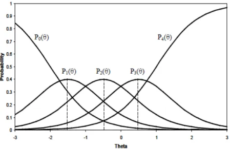
Figure 2.2 Category Response Curves for a 5-category Item under the GR Model

For this 5-categeory item, there are 5 category response curves showed in Figure 2.2. The curve for the lowest category (0) is monotonically decreasing, whereas, the curve for the highest category (4) is monotonically increasing. The curves for the middle three categories (1, 2, and 3)

are bell-shaped. Under the GR model, the slope parameter determines the shape of these curves for the middle categories: the higher the slope parameter, the narrower and more peaked the curves. The threshold parameters determine the locations of the curves for the middle response categories. Specifically, these category response curves peak in the middle of two adjacent threshold parameters. As showed using dashed lines in Figure 2.2, the middle value of two threshold values (b1 = -2 and b2 = -1) is -1.5 which is the mode of the curve for category score 1.

2.1.3 Main Threats in Applying Unidimensional IRT Models to PAs

Due to the well-known advantages of IRT over classical test theory (CTT), IRT has become main-stream for analyzing item response data in educational and psychological measurement. However, IRT is based on many strong assumptions such as dimensionality, local independence, and model-data fit. The inferences about the applications of any IRT model are valid only when all the underlying assumptions for that model are met. Therefore, before any accurate inference is drawn, it is necessary to check the assumptions in order to validate applications of IRT models. It is especially true when unidimensional polytomous IRT models are applied for performance assessments because the assumptions are more likely to be violated due to the properties of performance tasks. This section discusses some main threats in applying unidimensional IRT models to performance assessments.

2.1.3.1Multidimensionality

Most of the commonly used IRT models assume that one ability dimension determines examinees’ performance. However, the constructs measured in performance assessments are very likely to be multidimensional and this multidimensionality is mainly due to the complexity

of performance tasks. Performance tasks are typically developed to measure the complex structure of multiple skills and knowledge needed for solving more realistic problems. Thus, each item in performance assessments usually measures several dimensions simultaneously. For example, a mathematics problem might focus on problem-solving and communication abilities. In order to do well on that problem, students must be able to not only solve the problem, but also communicate their ideas clearly.

Another case is that large-scale performance assessments usually cover a broad range of content areas. For example, a math assessment may measure two content areas: algebra and geometry. Though this test measures student’s overall math ability and a unidimensional IRT model is commonly applied, the responses to this test is actually 2-dimensional.

In addition to this planned content structure, many nuisance or construct-irrelevant factors would result in multidimensionality for performance assessments. For example, a performance assessment intended to measure only mathematics ability might also require examinee reading ability. When there is variability on reading ability among the examinees, the reading ability would be viewed as nuisance dimension. Moreover, performance tasks are designed to be contextual or have real-life applications. The degree to which a student is familiar with a specific context would affect his/her performance. If the context effect varies across examinees, it would introduce an additional nuisance dimension. Furthermore, performance tasks often take more time to respond, and if the testing time was inadequate for some examinees, “speededness” would result in another potential construct-irrelevant dimension.

Finally, performance tasks are typically combined with multiple-choice items in order to measure examinees’ abilities more accurately. The combination of different item formats would

result in multidimensionality because different formats might measure different level of cognitive processing (Lane & Stone, 2006; Tate, 2002).

In summary, multidimensionality in item responses for performance assessments can be easily caused by various factors such as planed test construct structure, unintended nuisance or construct-irrelevant variances, and mixed item format. Unfortunately, in many practical situations, this multidimensionality is completely ignored and the unidimensional models are often applied to performance assessments. The lack of applications of multidimensional IRT (MIRT) models is due to the difficulties in parameter estimation and the interpretation of the latent ability space, as well as no user-friendly software available for estimating MIRT models (DeAyala, 1994).

When a unidimensional IRT model is used to fit multidimensional data, several problems might arise. Several researchers (Ackerman, 1989; Ansley & Forsyth, 1985, Way, Ansley, & Forsyth, 1988) have investigated the consequences of fitting 2-dimensional dichotomous item data with unidimensional three-parameter logistic (3PL) models and found violations of the unidimensionality assumption clearly affected IRT parameter estimates. DeAyala (1994, 1995) extended the previous work on the influence of multidimensionality on dichotomous model parameter estimation to polytomous models including the GR model and the PC model. For example, it was found that for the GR model, the difficulty parameters were well estimated, the discrimination estimate more accurately estimated the average discrimination than either dimensional a1 or a2, and the single ability estimate also estimated the average more accurately than either dimensional ability. Using incorrect model parameter estimates would subsequently affect IRT applications such as equating, CAT, as well as the validity of ability score interpretations. Tate (2002) summarized the previous studies and discussed that unidimensional

ability estimates represent a target composite of abilities, and is only robust to violations of the unidimensional assumption when the correlations among ability dimensions are moderate or high. Otherwise, the validity of any inferences from the single ability estimate will be threatened and it may not be appropriate to use unidimensional model (Lane & Stone, 2006).

Reckase (1985) found that difficulty and dimensionality can be confounded in the data and thus the composite of abilities does not remain consistent across the ability scale. For example, if the easy items measured one ability and the hard items measured another ability, low and high scores on the ability scale would not have the same meaning as could be a serious threat to validity of the total score. In addition, Ackerman (1992) demonstrated how the items may display differential item functioning (DIF) if unidimensional model is used to scale multidimensional data. Walker and Beretvas (2001, 2003) found the open-ended items in a large-scale mathematics test functioned differentially in favor of students who were highly capable of communicating their ideas and they further explored the effect of using only a single score on student proficiency classifications in mathematics. Their results indicated that when data believed to be multidimensional are modeled using a unidimensional model, different inferences may be made about student proficiency. Examinees having less mathematics communication ability were more likely to be placed in a lower general mathematics proficiency classification under the unidimensional than multidimensional model.

2.1.3.2Local Dependence

Local independence (LI) is a fundamental assumption for IRT models which means that there is no relationship between examinees responses to different items after accounting for trait abilities measured by a test. This conditional independence can be expressed mathematically as:

(

)

∏

(

)

= = = = I i i i x X P P 1 | |θ θ x X . (2.4) It describes that the probability of any pattern of responses to all items (x), conditioned on the abilities (θ), is equal to the product of the conditional probabilities of the response to each item. This equation defines the strong form of local independence. A weak form of local independence was proposed by McDonald (1979): the conditional covariances of all pairs of item responses on the abilities are equal to zero. When this assumption is met, the joint probability of responses to an item pair, conditioned on the abilities, is the product of the probabilities of responses to these two items,

P

(

X_i = x_i,X_j =x_j |θ

)

=P

(

X_i =x_i |θ

)

P

(

X_j =x_j |θ

)

. (2.5) This is a weaker form because higher-order dependencies among items are allowed.

An even weaker form of local independence was proposed by Stout (1987) who called it as “essential item independence” and defined it as “the items in a test can be considered as essentially independent when the average value of the conditional covariances between items approaches zero as test length increases for all ability values”. It is a weakest form of local independence since it only requires the average value of covariances rather than all covariances close to 0.

A number of researchers have discussed that the local independence assumption is related to the dimensionality assumption. The strong form indicates that the abilities measured by a test completely explain the difference on examinees’ performances. The weak local independence implies that the abilities completely explain the covariance between all item pairs between all item pairs. Finally the essential independence implies that the abilities dominate the difference on examinees’ performances (Yen & Fitzpatrick, 2006).

The potential presence of local dependence (LD) may be a more related issue to performance assessments (PA) than multiple-choice (MC) assessments. In MC tests, the items are usually carefully designed to be independent of one another. In contrast, a setting or context related to a real life situation is usually established in PA and students are asked several questions related to that setting (Yen, 1993). Yen (1993) discussed several potential sources of LD in PA such as: external assistance or interference with some items, speededness, fatigue, practice, special item or response format, a shared stimulus or passage, item chaining, items requiring explanation of a previous answer, scoring rubrics or raters, unique content knowledge or abilities, and differential opportunity to learn. Most of these sources reflect an additional nuisance factor (person, item, or rater characteristics) that consistently affects the performance of some students on some items to a great extent, and some sources reflect item interactions such as item chaining and a shared stimulus (Lane & Stone, 2006; Yen, 1993). Several studies (Yen, 1993; Ferrara, Huynh, & Baghi, 1997; Ferrara, Huynh, & Michaels, 1999) have showed some sources of LD can cause very strong empirical LD.

IRT models are not robust to the violation of local independence assumption. Applying an IRT model to LD response data could cause serious problems. First, the parameter estimates may be biased because the likelihood function for IRT models is based on local independence assumption and the incorrect likelihood would affect the accuracy of parameter estimation. Yen (1993) demonstrated that positive LD would produce higher item discriminations for LD items. Thus, the test information may be overestimated, and the standard errors of test scores would be underestimated. These effects would subsequently affect any application of IRT models. For example, the biased item discrimination estimates would affect item banking, and the underestimated standard errors would cause the premature termination in case of CAT.

In summary, the potential for violations in the assumptions of unidimensionality and local independence may be more likely for performance assessments and the consequences of these violations can not be ignored. Therefore, it is very important to check these two assumptions before a unidimensional IRT model is applied to a performance assessment data.

2.2 TRADITIONAL METHODS FOR CHECKING IRT MODEL-FIT

Assessing the fit of IRT models is a multi-facet procedure that often involves the collection of evidence about different aspects of fit: (1) assessing IRT model assumptions such as unidimensionality and local independence; (2) assessing the goodness-of-fit of IRT models at the item, person, and test levels (Embretson & Reise, 2000). A variety of methods have been proposed for assessing the corresponding different aspects of fit. This section reviews traditional approaches to checking the assumptions of unidimensionality and local independence and evaluating the goodness-of-fit at item level for polytomous IRT models because these three aspects are of the main interest in the present study.

2.2.1 Assessing Dimensionality

Several methods have been developed for assessing the dimensionality of polytomously scored items and most of them are polytomous extensions of methods for dichotomous item response. These methods fall into three categories: (1) factor analytic methods; (2) multidimensional IRT methods; (3) nonparametric methods.

Common linear factor analysis using Pearson product-moment correlations with maximum likelihood (ML) estimation can only be applied when the response scale for polytomous items has a large number of response categories and can be treated as a continuous interval scale. Several factor analytic methods have been proposed specifically for ordinal response data. For example, a weighted least square (WLS) analysis of polychoric correlations has been developed and can be implemented in PRELIS/LISREL (Joreskog & Sorbom, 2006) and Mplus (Muthén & Muthén, 2006). WLS requires a weight matrix which involves the inverse of the covariance matrix of polychoric correlations. The size of the weight matrix is usually substantial and it grows dramatically as the number of items increases. As a result, an adequate estimate of the weight matrix requires a very large sample size. When the sample size is small or moderate, a robust WLS approach (Muthén, duToit, & Spisic, 1997) is considered as the best approach for factor analysis of ordinal variables. The robust WLS approach uses the identity matrix rather than the weight matrix and its estimation does not require extensive computation and enormously large sample sizes. Two robust WLS methods (mean-adjusted WLS and mean- and variance-adjusted WLS) are available in Mplus. In a simulation study, Flora and Curren (2004) showed that WLS performed adequately only at the largest sample size but led to substantial estimation difficulties with smaller samples, whereas, the robust WLS performed well across all simulation conditions.

Compared with factor analytic methods, MIRT approaches use all information in response patterns rather than limited information from correlation matrices. A full-information item factor analysis for polytomous item responses was proposed by Muraki and Carlson (1995) and this method can be implemented in the most recent version of PRELIS/LISREL (Joreskog & Sorbom, 2006). Another is a Rasch MIRT modeling approach proposed by Adams, Wilson, and

Wang (1997) which assumes the slope or discrimination parameter is constant across all items. This method is available in ConQuest (Wu, Adams, & Wilson, 1998).

The unidimensionality assumption indicates that there is a single latent ability measured by a particular test. However, a real-world test will never be strictly unidimensional. Given this fact, Stout (1987) proposed the concept of “essential unidimensionality” for a test which measures a dominant dimension and examinees’ performances are unaffected by the presence of minor dimensions. This concept is directly related to “essential local independence” discussed in section 2.1.3.2. To assess whether a test is essential unidimensional for applying a unidimensional IRT model, nonparametric approaches have been developed by Stout and his colleagues (1987, 1990, 1993, & 1996) based on conditional item covariance theory. The simple hypothesis that a test is essentially unidimensional can be examined using DIMTEST software (Nandakumar & Stout, 1993). Poly-DIMTEST (Nandakumar, Yu, Li, & Stout ,1998) is an extension of DIMTEST to accommodate tests that contain polytomous items. DETECT program (Zhang & Stout, 1999) provides more information than DIMTEST by estimating the extent of multidimensional approximate simple structure in a test. Poly-DETECT (Yu & Nandakumar, 2001) is a polytomous extension of DETECT. In addition, HCC/CCPROX program (Roussos, Stout, & Marden, 1998) is used to search dimensionally homogeneous clusters of items using hierarchical cluster analysis technique, and its polytomous version is Poly-CCPROX/HCA (Tay-Lim & Stone, 2000).

2.2.2 Detecting Local Dependence

The IRTNEW software (Chen, 1998) provides five different measures of item local dependence (LD) for dichotomous items. All of them are IRT based and examine LD in the context of