Accurate Estimation of Isoform and Gene Expression Levels from Next Generation Sequencing Data

(1)

University of Connecticut

OpenCommons@UConn

Master's Theses University of Connecticut Graduate School

9-16-2011

Accurate Estimation of Isoform and Gene

Expression Levels from Next Generation

Sequencing Data

Marius Nicolae

University of Connecticut - Storrs, [email protected]

This work is brought to you for free and open access by the University of Connecticut Graduate School at OpenCommons@UConn. It has been accepted for inclusion in Master's Theses by an authorized administrator of OpenCommons@UConn. For more information, please contact

[email protected].

Recommended Citation

Nicolae, Marius, "Accurate Estimation of Isoform and Gene Expression Levels from Next Generation Sequencing Data" (2011). Master's Theses. 187.

(2)

Accurate Estimation of Isoform and Gene

Expression Levels from Next Generation

Sequencing Data

Marius Nicolae

Dipl.-Ing. Computer Science, University POLITEHNICA of Bucharest, Romania, 2009

A Thesis

Submitted in Partial Fulfillment of the Requirements for the Degree of

Master of Science at the

University of Connecticut 2011

(3)

APPROVAL PAGE

Master of Science Thesis

Accurate Estimation of Isoform and Gene

Expression Levels from Next Generation

Sequencing Data

Presented by

Marius Nicolae, Dipl.-Ing.

Major Advisor Dr. Ion M˘andoiu Associate Advisor Dr. Sanguthevar Rajasekaran Associate Advisor Dr. Yufeng Wu University of Connecticut 2011

(4)

ACKNOWLEDGEMENTS

I would like to thank my major advisor Dr. Ion M˘andoiu and collaborators Dr. Alexander Zelikovsky and Serghei Mangul for their direct contributions to this thesis. Special acknowledgements go to professor Doru Popescu-Anastasiu, my high-school Computer Science teacher, who was a great inspiration for me and played a key role in me getting to UConn. I would also like to thank my associate advisors, professors, colleagues, friends and family for their support.

(5)

Ch. 2 : Accurate Estimation of Gene Expression Levels from DGE Se-quencing Data. . . 36 2.1. Introduction . . . 36 2.2. DGE Protocol . . . 38 2.3. DGE-EM Algorithm . . . 40 2.3.1. E-Step . . . 43 2.3.2. M-Step . . . 43 2.3.3. Inferringp . . . 44 2.3.4. Implementation . . . 45 2.4. Results . . . 46 2.4.1. Experimental Setup . . . 46

2.4.2. DGE-EM Outperforms Uniq . . . 48

2.4.3. Comparison of DGE and RNA-Seq Protocols . . . 49

2.4.4. Possible DGE Assay Optimizations . . . 50

2.5. Conclusions . . . 52

(6)

Introduction

Massively parallel transcriptome sequencing is quickly replacing microarrays as the technology of choice for performing gene expression profiling due to its wider dynamic range and digital quantitation capabilities. However, accu-rate estimation of expression levels from sequencing data remains challenging due to the short read length delivered by current sequencing technologies and still poorly understood protocol- and technology-specific biases. To date, two main transcriptome sequencing protocols have been proposed in the lit-erature. The most commonly used one, referred to as RNA-Seq, generates short (single or paired) sequencing tags from the ends of randomly generated cDNA fragments. An alternative protocol, referred to as 3’-tag Digital Gene Expression (DGE), or high-throughput sequencing based Serial Analysis of Gene Expression (SAGE-Seq), generates single cDNA tags using an assay in-cluding as main steps transcript capture and cDNA synthesis using oligo(dT) beads, cDNA cleavage with an anchoring restriction enzyme, and release of cDNA tags using a tagging restriction enzyme whose recognition site is ligated upstream of the recognition site of the anchoring enzyme.

(7)

inference of isoform- and/or gene-specific expression levels from RNA-Seq and DGE data and a comparison of estimation performance of the two transcrip-tome sequencing protocols.

The first algorithm, IsoEM [1, 3], works on RNA-Seq data and is based on disambiguating of information provided by the distribution of insert sizes generated during sequencing library preparation and takes advantage of base quality scores, strand and read pairing information when available. Empirical experiments on both synthetic and real RNA-Seq datasets show that IsoEM has scalable running time and outperforms existing methods of isoform and gene expression level estimation. Simulation experiments confirm previous findings that, for a fixed sequencing cost, using reads longer than 25-36 bases does not necessarily lead to better accuracy for estimating expression levels of annotated isoforms and genes.

The second chapter introduces a rigorous statistical model of DGE data and a novel expectation-maximization algorithm, DGE-EM [2], for inference of gene and isoform expression levels from DGE tags. Unlike previous methods, our algorithm takes into account alternative splicing isoforms and tags that map at multiple locations in the genome, and corrects for incomplete digestion and sequencing errors. Experimental results show that DGE-EM outperforms methods based on unique tag counting on a multi-library DGE dataset con-sisting of 20bp tags generated from two commercially available reference RNA samples that have been well-characterized by quantitative real time PCR as

(8)

part of the MicroArray Quality Control Consortium (MAQC).

We also take advantage of the availability of RNA-Seq data generated from the same MAQC samples to directly compare estimation performance of the two transcriptome sequencing protocols. While RNA-Seq is clearly more powerful than DGE at detecting alternative splicing and novel transcripts such as fused genes, previous studies have suggested that for gene expression profiling DGE may yield accuracy comparable to that of RNA-Seq at a fraction of the cost [38]. We find that the two protocols achieve similar cost-normalized accuracy on the MAQC samples when using state-of-the-art estimation methods. However, the current protocol versions are unlikely to be optimal. Indeed, the results of a comprehensive simulation study assessing the effect of various experi-mental parameters suggest that further improvements in DGE accuracy could be achieved by using anchoring enzymes with degenerate recognition sites and using partial digest of cDNA with the anchoring enzyme during library preparation.

(9)

Chapter 1 Estimation of alternative splicing isoform

frequencies from RNA-Seq data

1.1 Background

Ubiquitous regulatory mechanisms such as the use of alternative transcription start and polyadenylation sites, alternative splicing, and RNA editing result in multiple messenger RNA (mRNA) isoforms being generated from a single genomic locus. Most prevalently, alternative splicing is estimated to take place for over 90% of the multi-exon human genes across diverse cell types [33], with as much as 68% of multi-exon genes expressing multiple isoforms in a clonal cell line of colorectal cancer origin [11]. Not surprisingly, the ability to reconstruct full length isoform sequences and accurately estimate their expression levels is widely believed to be critical for unraveling gene functions and transcription regulation mechanisms [25].

Three key interrelated computational problems arise in the context of tran-scriptome analysis: gene expression level estimation (GE), isoform expression level estimation (IE), and novel isoform discovery (ID). Targeted GE using methods such as quantitative PCR has long been a staple of genetic studies. The

(10)

com-pletion of the human genome has been a key enabler for genome-wide GE performed using expression microarrays. Since expression microarrays have limited capability of detecting alternative splicing events, specialized splicing arrays have been developed for genome-wide interrogation of both annotated exons and exon-exon junctions. However, despite sophisticated deconvolution algorithms [4, 28], the fragmentary information provided by splicing arrays is typically insufficient for unambiguous identification of full-length transcripts [14, 18]. Massively parallel whole transcriptome sequencing, commonly re-ferred to as RNA-Seq, is quickly replacing microarrays as the technology of choice for performing GE due to their wider dynamic range and digital quan-titation capabilities [34]. Unfortunately, most RNA-Seq studies to date still ignore alternative splicing or, similar to splicing array studies, restrict them-selves to surveying the expression levels of exons and exon-exon junctions. The main difficulty in inferring expression levels for full-length isoforms lies in the fact that current sequencing technologies generate short reads (from few tens to hundreds of bases), many of which cannot be unambiguously assigned to individual isoforms.

1.1.1 Related work

RNA-Seq analyses typically start by mapping sequencing reads onto the refer-ence genome, transcript libraries, exon-exon junction libraries, or combinations thereof. Early RNA-Seq studies have recognized that limited read lengths result

(11)

in a significant percentage of so calledmultireads, i.e., reads that map equally well at multiple locations in the genome. A simple (and still commonly used) approach is to discard multireads, and estimate expression levels using only the so called unique reads. Mortazavi et al. [22] proposed a multiread “res-cue” method whereby initial gene expression levels are estimated from unique reads and used to fractionally allocate multireads, with final expression levels obtained by re-estimation based on total counts obtained after multiread allo-cation. An expectation-maximization (EM) algorithm that extends this scheme by repeatedly alternating between fractional read allocation and re-estimation of gene expression levels was recently proposed in [24].

A number of recent works have addressed the IE problem, namely isoform expression level estimation from RNA-Seq reads. Under a simplified “exact information” model, [18] showed that neither single nor paired read RNA-Seq data can theoretically guarantee unambiguous inference of isoform expression levels, although paired reads may be sufficient to deconvolute expression lev-els for the majority of annotated isoforms. The key challenge in IE is accurate assignment of ambiguous reads to isoforms. Compared to the GE context, read ambiguity is much more significant, since it affects not only multireads, but also reads that map at a unique genome location expressed in multiple isoforms. Estimating isoform expression levels based solely on unambiguous reads, as suggested, e.g., in [11], results in splicing-dependent biases similar to the transcript-length bias noted in [23], further complicating the design of

(12)

unbiased differential expression tests based on RNA-Seq data. To overcome this difficulty, [17] proposed a Poisson model of single-read RNA-Seq data explicitly modeling isoform frequencies. Under their model, maximum like-lihood estimates are obtained by solving a convex optimization problem, and uncertainty of estimates is obtained by importance sampling from the posterior distribution. Li et al. [20] introduced an expectation-maximization (EM) algo-rithm similar to that of [24] but applied to isoforms instead of genes. Unlike the method of [17], which estimates isoform frequencies only from reads that map to a unique location in the genome, the algorithm of [20] incorporates multireads as well. The IE problem for single reads is also tackled in [26], who propose an EM algorithm for inferring isoform expression levels from the read coverage of exons (reads spanning exon junctions are ignored).

The related novel isoform discovery (ID) problem is also receiving much in-terest in the literature. Although showing encouraging results, de novo tran-scriptome assembly algorithms such as [5, 16, 30] have difficulties in identify-ing transcripts with moderate coverage. Very recently, [10, 12, 32] proposed genome-assisted (i.e., mapping based) methods for simultaneously solving ID and IE based on paired RNA-Seq reads. The method of Feng et al. [10] gener-ates isoform candidgener-ates from the splicing graph derived from annotations and reads spanning exon-exon junctions. After discarding multireads, [10] formu-lates IE for a given set of isoforms as a convex quadratic program (QP) that can be efficiently solved for each gene locus. The set of isoform candidates is

(13)

iteratively refined until thep-value of the objective value of the QP, assumed to follow a χ2 _{distribution, exceeds an empirically selected threshold of 5%.}

Pair read information is not directly used in isoform frequency estimation, contributing only as secondary data to filter out false positives in the process of isoform selection. As in [10], Guttman et al. [12] construct a splicing graph from the mapped reads and filter candidate isoforms using paired-end information. Isoform specific expression levels are inferred using the method of [22]. After performing spliced alignment of (paired) reads onto the genome using TopHat [31], the method of Trapnell et al. [32], referred to as Cufflinks, constructs a read overlap graph and generates candidate isoforms by finding a minimal size path cover via a reduction to maximum matching in a weighted bipartite graph. Reads that match equally well multiple locations in the genome are fractionally allocated to these locations, and estimation is then performed in-dependently at different transcriptional loci, using an extension to paired reads of the methods in [17].

1.1.2 Our contributions

In this chapter we focus on the IE problem, namely estimating isoform expres-sion levels (interchangeably referred to as frequencies) from RNA-Seq reads, under the assumption that a complete list of candidate isoforms is available. Projects such as [7] and [21] have already assembled large libraries of full-length cDNA sequences for humans and other model organisms, and the coverage of

(14)

these libraries is expected to continue to increase rapidly following ultra-deep paired-end transcriptome sequencing projects such as [12, 32] and the widely anticipated deployment of third-generation sequencing technologies such as [8, 9], which deliver reads with significantly increased length. Inferring ex-pression at isoform level provides information for finer-resolution biological studies, and also leads to more accurate estimates of expression at the gene level by allowing rigorous length normalization. Indeed, as shown in the ‘Experimental results’ section, genome-wide gene expression level estimates derived from isoform level estimates are significantly more accurate than those obtained directly from RNA-Seq data using isoform-oblivious GE methods such as the widely used counting of unique reads, the rescue method of [22], or the EM algorithm of [24].

Our main contribution is a novel expectation-maximization algorithm for iso-form frequency estimation from any mixture of single and paired RNA-Seq reads. A key feature of our algorithm, referred to as IsoEM, is that it ex-ploits information provided by the distribution of insert sizes, which is tightly controlled during sequencing library preparation under current RNA-Seq pro-tocols. Such information is not modeled in the “exact” information models of [14, 18], challenging the validity of their negative results. Guttman et al. [12] take into account insert lengths derived from paired read data, but only for filtering candidate isoforms in ID. Trapnell et al. [32] is the only other work we are aware of that exploits this information for IE, in conjunction with paired

(15)

read data. We show that modeling insert sizes is highly beneficial for IE even for RNA-Seq data consisting of single reads. Insert sizes contribute to increased estimation accuracy in two different ways. On one hand, they can help dis-ambiguating the isoform of origin for the reads. In IsoEM, insert lengths are combined with base quality scores, and, if available, read pairing and strand information to probabilistically allocate reads to isoforms during the expecta-tion step of the algorithm. As in [20], the genomic locaexpecta-tions of multireads are also resolved probabilistically in this step, further contributing to improved overall accuracy compared to methods that ignore or fractionally pre-allocate multireads. On the other hand, insert size distribution is used to accurately ad-just isoform lengths during frequency re-estimation in the maximization step of the IsoEM algorithm.

We also present the results of comprehensive experiments conducted to assess the performance of IsoEM on both synthetic and real RNA-Seq datasets. These results show that IsoEM consistently outperforms existing methods under a wide range of sequencing parameters and distribution assumptions. We also report results of experiments empirically evaluating the effect of sequencing parameters such as read length, read pairing, and strand information on esti-mation accuracy. Our experiments confirm the surprising finding of [20] that, for a fixed total number of sequenced bases, longer reads do not necessarily lead to better accuracy for estimation of isoform and gene expression levels.

(16)

1.2 Methods

1.2.1 Read mapping

As with many RNA-Seq analyses, the first step of IsoEM is to map the reads. Our approach is to map them onto the library of known isoforms using any one of the many available ungapped aligners (we used Bowtie [19] with default parameters in our experiments). An alternative strategy is to map the reads onto the genome using a spliced alignment tool such as TopHat [31], as done, e.g., in [12, 32]. However, preliminary experiments with TopHat resulted in fewer mapped reads and significantly increased mapping uncertainty, despite providing TopHat with a complete set of annotated junctions. Since further increases in read length coupled with improvements in spliced alignment algo-rithms could make mapping onto the genome more attractive in the future, we made our IsoEM implementation compatible with both mapping approaches by always converting read alignments to genome coordinates and performing all IsoEM read-isoform compatibility calculations in genome space.

1.2.2 Finding read-isoform compatibilities

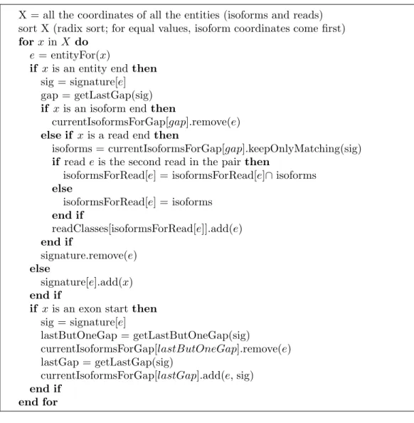
The candidate set of isoforms for each read is obtained by combining all genome coordinates of reads and isoforms, sorting them and using a line sweep tech-nique to detect read-isoform compatibilities (see Figure 1.2.1) As detailed be-low, during the line sweep reads are grouped into equivalence classes defined by their isoform compatibility sets; this speeds up the E-step of the IsoEM

(17)

algorithm by allowing the processing of an entire read class at once.

Some of the reads match multiple positions in the genome, which we refer to as

alignments(for paired end reads, an alignment consists of the positions where the two reads in the pair align with the genome). Each alignment a can in turn be compatible with multiple isoforms that overlap at that position of the genome. During the line sweep, we compute the relative “weight” of assigning a given read/pairrto isoform jaswr,j = PaQaFaOa, where the sum is over all

alignments ofrcompatible with j, and the factors of the summed products are defined as follows:

• Qa represents the probability of observing the read from the genome

locations described by the alignment. This is computed from the base quality scores asQa =

Q|r|

k=1[(1−εk)Mak +

εk

3(1−Mak)], where Mak = 1 if

positionk of alignment amatches the reference genome sequence and 0 otherwise, whileεkdenotes the error probability ofk-th base ofr.

• For paired end reads,Farepresents the probability of the fragment length

needed to produce alignmentafrom isoform j; note that the length of this fragment can be inferred from the genome coordinates of the two aligned reads and the available isoform annotation. For single reads, we can only estimate an upperbounduon the fragment length: if the alignment is on the same strand as the isoform thenuis the number of isoform annotated bases between the 5′_{end of the aligned read and the 3}′_{end of the isoform,}

(18)

otherwiseuis the number of isoform annotated bases between the 5′_end

of the aligned read and the 5′_{end of the isoform. In this case}_F

ais defined

as the probability of observing a fragment with length ofubases or fewer.

• Oa is 1 if alignmentaofr is consistent with the orientation of isoform j,

and 0 otherwise. Consistency between the orientations ofrandjdepends on whether or not the library preparation protocol preserves the strand information. For single reads Oa = 1 when reads are generated from

fragment ends randomly or, for directional RNA-Seq, when they match the known isoform orientation. For paired-end reads,Oa = 1 if the two

reads come from different strands, point to each other, and, in the case of directional RNA-Seq, the orientation of first read matches the known isoform orientation.

1.2.3 The IsoEM algorithm

The IsoEM algorithm starts with the set ofNknown isoforms. For each isoform we denote byl(j) its length and by f(j) its (unknown) frequency. If we denote by n(j) the number of reads coming from isoform j and let p(k) denote the probability of a fragment of lengthk, then

E[n(j)]∝ X

k≤l(j)

p(k)(l(j)−k+1) (1.2.1)

since, the number of fragments of length k is expected to be proportional to the number of valid starting positions for a fragment of that length in the

(19)

X = all the coordinates of all the entities (isoforms and reads) sort X (radix sort; for equal values, isoform coordinates come first)

for_x_in_X do

e = entityFor(x)

if _x_{is an entity end}then

sig = signature[e] gap = getLastGap(sig)

if x is an isoform endthen

currentIsoformsForGap[gap].remove(e)

else if _x _{is a read end}then

isoforms = currentIsoformsForGap[gap].keepOnlyMatching(sig)

if _read_e _{is the second read in the pair}then

isoformsForRead[e] = isoformsForRead[e]∩isoforms

else isoformsForRead[e] = isoforms end if readClasses[isoformsForRead[e]].add(e) end if signature.remove(e) else signature[e].add(x) end if

if _x_{is an exon start}then

sig = signature[e]

lastButOneGap = getLastButOneGap(sig)

currentIsoformsForGap[lastButOneGap].remove(e) lastGap = getLastGap(sig)

currentIsoformsForGap[lastGap].add(e, sig)

end if end for

Figure 1.2.1: The algorithm for identifying isoforms compatible with reads.

isoform. Thus, if the isoform of origin is known for each read, the maximum likelihood estimator for f(j) is given by c(j)/(c(1)+_{. . .}+c(N)), where c(j) =

n(j)/P

k≤l(j)p(k)(l(j)−k+1) denotes the length-normalized fragment coverage.

Note that the length of most isoforms is significantly larger than the mean fragment length µ typical of current sequencing libraries; for such isoforms

P

k≤l(j)p(k)(l(j)−k+1)≈l(j)−µ+1 andc(j) can be approximated byn(j)/(l(j)−

(20)

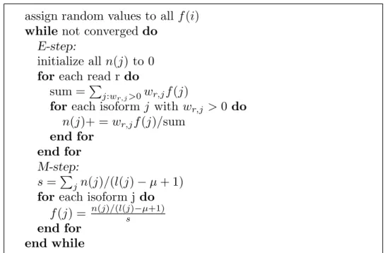
Since some reads match multiple isoforms, their isoform of origin cannot be established unambiguously. The IsoEM algorithm (see Figure 1.2.2) overcomes this difficulty by simultaneously estimating the frequencies and imputing the missing read origin within an iterative framework. After initializing frequen-cies f(j) at random, the algorithm repeatedly performs the next two steps until convergence:

• E-step: Compute the expected number n(j) of reads that come from isoform junder the assumption that isoform frequencies f(j) are correct, based on weightswr,j computed as described in the previous section

• M-step: For each j, set the new value of f(j) to c(j)/(c(1)+. . .+c(N)), where normalized coveragesc(j) are based on expected counts computed in the prior E-step

1.2.4 IsoEM optimizations

Below we describe two implementation optimizations that significantly im-prove the performance of IsoEM by reducing both runtime and memory usage. The first optimization consists of partitioning the input into compatibility com-ponents. The compatibility between reads and isoforms naturally induces a bipartite read-isoform compatibility graph, with edges connecting each isoform with all reads that can possibly originate from it. Connected components of the compatibility graph can be processed independently in IsoEM since the fre-quencies of isoforms in one connected component do not affect the frequencies

(21)

assign random values to all f(i)

while _{not converged}do

E-step:

initialize all n(j) to 0

for _{each read r} do

sum =P_j_:_w_r,j_>₀wr,jf(j)

for _{each isoform}_j _with _w_r,j _>₀do

n(j)+ =wr,jf(j)/sum

end for end for

M-step:

s=P_jn(j)/(l(j)−µ+ 1)

for _{each isoform j} do

f(j) = n(j)/(l(j)−µ+1)

s

end for end while

Figure 1.2.2: The expectation-maximization algorithm used by IsoEM.

of isoforms in any other connected component. Although this optimization can be applied to any EM algorithm, its impact is particularly significant in IsoEM. Indeed, in this context the compatibility graph decomposes in numerous small components (see Figure 1.2.3(a) for a typical distribution of component sizes; a similar distribution of component sizes is reported for Arabidopsis gene mod-els in [15]). The resulting speed-up comes from the fact that in each iteration of IsoEM we update frequencies of isoforms in a single compatibility component, avoiding needless updates for other isoforms.

The second IsoEM optimization consists of partitioning the set of reads within each compatibility component into equivalence classes. Two reads are equiv-alent for IsoEM if they are compatible with the same set of isoforms and their compatibility weights to the isoforms are proportional. Keeping only a single

(22)

10,000 1,000 10,000 100 1,000 10,000 C o m p o n e ts 100 1,000 10,000 N u m b e r o f C o m p o n e ts 10 100 1,000 10,000 N u m b e r o f C o m p o n e ts 1 10 100 1,000 10,000 0 20 40 60 80 100 120 140 160 180 N u m b e r o f C o m p o n e ts

Component Size (# isoforms)

1 10 100 1,000 10,000 0 20 40 60 80 100 120 140 160 180 N u m b e r o f C o m p o n e ts

Component Size (# isoforms)

1 10 100 1,000 10,000 0 20 40 60 80 100 120 140 160 180 N u m b e r o f C o m p o n e ts

Component Size (# isoforms) (a) 0.4 0.6 0.8 1 1.2 C la ss e s (M il li o n s) RandomStrand Single CodingStrandSingle CodingStrand Pairs RandomStrand Pairs 0 0.2 0.4 0.6 0.8 1 1.2 0 5 10 15 20 25 30 # C la ss e s (M il li o n s) #Reads/Pairs(Millions) RandomStrand Single CodingStrandSingle CodingStrand Pairs RandomStrand Pairs (b)

Figure 1.2.3: Distribution of compatibility component sizes (defined as the number of isoforms) for 10 million single reads of length 75 (a) and number of read classes for 1 to 30 million single reads or pairs of reads of length 75 (b).

E-step for read classes:

initialize all n(j) to 0

for _{each read class} _R do

sum = P_j_:_w_R,j_>₀wR,jf(j)

for _{each isoform} _j _with _w_R,j _> ₀ do

n(j)+ = m(R)∗wR,jf(j)/sum

end for end for

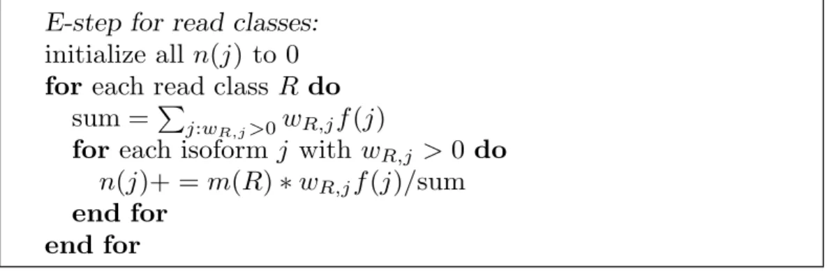
Figure 1.2.4: The E-Step of IsoEM algorithm based on read classes.

representative from each read class (with appropriately adjusted frequency) drastically reduces the number of reads kept in memory (see Figure 1.2.3(b)). As the number of reads increases, the number of read classes increases much slower. Eventually this reaches saturation and no new read classes appear – at which point the runtime of IsoEM becomes virtually independent of the number of reads. Indeed, in practice the runtime bottlenecks are parsing the reads, computing the compatibility graph and detecting equivalent reads.

(23)

E-step of IsoEM to use read classes instead of reads (Figure 1.2.4). Next we describe the union-find algorithm used for efficiently finding compatibility components and read classes in IsoEM. A read class is defined ashm,{(i,w)|i=

isoform,w = weight}i, where m is called the multiplicity of the read class. Given a collection of reads, we want to:

• Find the connected components of the compatibility graph induced by the reads, and

• Collapse equivalent reads into read classes with multiplicity indicating the number of reads in each class.

A straightforward approach is to solve the first problem using a union-find algorithm, then to take the reads corresponding to each connected component and remove equivalent reads, e.g., using hashing. However, there are two drawbacks to this approach:

• First, all reads need to be kept in memory until all connected components have been computed.

• Second, when the number of reads in a connected component is very large the number of collisions increases, which leads to poor performance.

We overcome the two problems presented above using an online version of the union-find algorithm which computes connected components and eliminates equivalent reads on the fly. This way, equivalent reads will never reside too

(24)

long in memory. Also, we avoid the problem of large hash tables by using multiple smaller hash tables which are guaranteed to be disjoint.

We start our modified version of union-find with an empty set of trees. A new single-node tree is initialized every time a new isoform is found in a read class. In each node we store a hash-table of read classes. Each read is processed as follows:

• If the isoforms compatible with the read correspond to nodes in more than one treeunite the corresponding trees. The root of the tallest tree becomes the root of the union tree. Then create a new read class for this read (we can be sure it was not seen before, otherwise the isoforms would have been in the same tree) and add it to the hash table of the root node. Notice that at this point the root node is also (trivially) the Lowest Common Ancestor (LCA) of the nodes corresponding to the isoforms in the read class

• If the isoforms correspond to nodes in the same treefind the LCA of all these nodes. If the class of the read is present in the hash table of the LCA, increment its multiplicity and then drop the read. Otherwise, create a new read class and add it to the LCA’s hash table.

Notice that in the second case it suffices to look only in the LCA of the isoforms for an already existing read class. This follows immediately from the fact that we always add reads to the LCA of the nodes (isoforms) compatible with the read. Note that we cannot use path compression to speed up ‘find’ operations

(25)

because this would be altering the structure of existing trees. Thus, ‘find’ op-erations will take logarithmic (amortized) time. At the end of the algorithm, each tree in the union-find forest corresponds to a connected component. The read classes in each connected component are obtained by traversing the cor-responding tree and collecting all the read classes present in the nodes. At this point we are sure that all the read classes are distinct, so the collection process performs simple concatenations. To further speed up the collection process, we can safely use path compression as we traverse the trees, since we no longer care about the exact topology of the subtrees.

Runtime analysis. Each union operation takesO(1) time, so for a read with k

compatible isoforms we spend at most O(k) time doing unions. By always making the root of the taller tree to be the root of a union, we ensure that the height of any tree is not bigger thanO(logn) wheren is the number of nodes in the tree. Thus, finding the root of a node’s tree takesO(logn). For a read withkcompatible isoforms we spend at mostO(klogn) time processing it. The LCA of two nodes can be computed at constant overhead when performing find operations (by marking the nodes on the paths from isoforms to root). Collecting all the read classes is sped-up by using path compression. The whole collecting phase takes O(nα(n)) time where n is the total number of isoforms andα(n) is the inverse of the Ackermann function. Overall, forqreads with an average ofk isoforms per read and n total distinct isoforms, computing read classes and compatibility components using the modified union-find algorithm

(26)

takesO(qklogn+nα(n)) time.

1.2.5 Hexamer and repeat bias corrections

As noted in [13], some commonly used library preparation protocols result in biased sampling of fragments from isoforms due to the random hexamers used to prime reverse transcription. To correct for possible hexamer bias, we implemented a simple re-weighting scheme similar to that proposed in [13]. Each read is assigned a weightb(h) based on its first six bases and computed as follows. Given a set of mapped reads, let ˆpi be the observed distribution of

hexamers starting at position i (spanning positionsi toi+5) of all the reads. Thus, ˆpi(h) is the proportion of reads which have hexamerhat position iand

ˆ

p1(h) is the proportion of reads starting with hexamerh. Letlbe the read length.

We define the weightsbby:

b(h)= 1 6 Pl/2+3 i=l/2−2pˆi(h) 1 2( ˆp1(h)+pˆ2(h))

Since we already collapse equivalent reads into read classes, we can seam-lessly incorporate hexamer weights in the algorithm by slightly changing the definition of a read class’ multiplicity to m(R) = P

r∈Rb(h(r)), where h(r)

de-notes the starting hexamer of r. The effect of this correction procedure is to reduce (respectively increase) the multiplicity of reads with starting hexamers that are overrepresented (respectively under-represented) at the beginning of reads compared to the middle of reads. The underlying assumption is that

(27)

the average frequency with which a hexamer appears in the middle of reads is not affected by library preparation biases. Recent methods [27] further target biases in the bases surrounding the sequenced fragments in addition to those at read ends.

To avoid biases from incorrectly mapped reads originating from repetitive re-gions, IsoEM will also discard reads that overlap annotated repeats. When applying this correction, isoform lengths are automatically adjusted by sub-tracting the number of positions resulting in reads that would be discarded.

1.3 Experimental results

1.3.1 Comparison of methods on simulated datasets

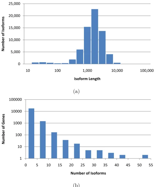
We tested IsoEM on simulated human RNA-Seq data. The human genome sequence (hg18, NCBI build 36) was downloaded from UCSC together with the coordinates of the isoforms in the KnownGenes table. Genes were defined as clusters of known isoforms defined by the GNFAtlas2 table. The dataset contains a total of 66,803 isoforms pertaining to 19,372 genes. The isoform length distribution and the number of isoforms per genes are shown in Figure 1.3.1.

Single and paired-end reads were randomly generated by sampling fragments from the known isoforms. Each isoform was assigned a true frequencybased on the abundance reported for the corresponding gene in the first human tissue of the GNFAtlas2 table, and a probability distribution over the isoforms

(28)

inside a gene cluster. Thus, the true frequency of isoform j isa(g)p(j), where

a(g) is the abundance of the gene g for which j is an isoform and p(j) is the probability of isoform j among all the isoforms of g. We simulated datasets with uniform, respectively truncated geometric distribution with ratior=1/2 for the isoforms of each gene. For a gene withkisoformsp(j)=1/k, j=1, . . . ,k, under the uniform distribution. Under the truncated geometric distribution, the respective isoform probabilities are p(j) = 1/2j for j = 1, . . . ,k −1 and

p(k) = 1/2k−1_{. Fragment lengths were simulated from a normal probability}

distribution with mean 250 and standard deviation 25.

We compared IsoEM to several existing algorithms for solving the IE and GE problems. For IE we included in the comparison the isoform analogs of the Uniq and Rescue methods used for GE [22], an improved version of Uniq (UniqLN) that estimates isoform frequencies from unique read counts but normalizes them using adjusted isoform lengths that exclude ambiguous positions, the Cufflinks algorithm of [32] (version 0.8.2), and the RSEM algorithm of [20] (version 0.6). For the GE problem, the comparison included the Uniq and Rescue methods, our implementation of the GeneEM algorithm described in [24], and estimates obtained by summing isoform expression levels inferred by Cufflinks, RSEM, and IsoEM. All methods use alignments obtained by mapping reads onto the library of isoforms with Bowtie [19] and then converting them to genome coordinates, except for Cufflinks which uses alignments obtained by directly mapping the reads onto the genome with TopHat [31], as suggested

(29)

in [32].

Frequency estimation accuracy was assessed using the coefficient of determi-nation, r2_{, along with the} _{error fraction (EF)} _and _{median percent error (MPE)}

measures used in [20]. However, accuracy was computed against true fre-quencies, not against estimates derived from true counts as in [20]. If ˆfi is the

frequency estimate for an isoform with true frequency fi, the relative error is

defined as|fˆi − fi|/fi if fi , 0, 0 if ˆfi = fi = 0, and ∞if ˆfi > fi = 0. The error

fraction with thresholdτ, denotedEFτis defined as the percentage of isoforms

with relative error greater or equal to τ. The median percent error, denoted MPE, is defined as the thresholdτfor whichEFτ =50%.

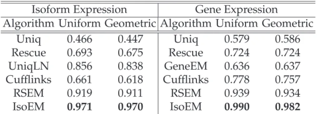
Since not all compared methods could handle paired reads or strand infor-mation we focused our comparisons on single read data. Table 1.3.1 gives

r2 values for isoform, respectively gene expression levels inferred from 30M reads of length 25, simulated assuming both uniform and geometric isoform expression. IsoEM significantly outperforms the other methods, achieving an

r2 _{values of over .96 for all datasets. For all methods the accuracy di}_ff_erence

between datasets generated assuming uniform and geometric distribution of isoform expression levels is small, with the latter one typically having a slightly worse accuracy. Thus, in the interest of space we present remaining results only for datasets generated using geometric isoform expression.

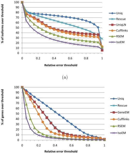
For a more detailed view of the relative performance of compared IE and GE algorithms, Figure 1.3.2 gives the error fraction at different thresholds ranging

(30)

between 0 and 1. The variety of methods included in the comparison allows us to tease out the contribution of various algorithmic ideas to overall estimation accuracy. The importance of rigorous length normalization is illustrated by the significant IE accuracy gain of UniqLN over Uniq – clearly larger than that achieved by ambiguous read reallocation as implemented in the IE version of Rescue. Proper length normalization is also explaining the accuracy gain of isoform-aware GE methods (Cufflinks, RSEM, and IsoEM) over isoform oblivious GE methods. Similarly, the importance of modeling insert sizes even for single read data is underscored by the significant IE and GE accuracy gains of IsoEM over RSEM. Indeed, the latest version of the RSEM package, released as this article goes to print, has been updated to include modeling of insert sizes and appears to have accuracy matching that of IsoEM.

For yet another view, Tables 1.3.2 and 1.3.3 report the MSE and EF.15 measures

for isoform, respectively gene expression levels inferred from 30M reads of length 25, computed over groups of isoforms with various expression levels. IsoEM consistently outperforms the other IE and GE methods at all expression levels except for isoforms with zero true frequency, where it is dominated by the more conservative Uniq algorithm and its UniqLN variant.

1.3.2 Comparison of methods on two real RNA-Seq datasets

In addition to simulation experiments, we validated IsoEM on two real RNA-Seq datasets. The first dataset consists of two samples with approximately 8

(31)

million 27bp Illumina reads each, generated from two human cell lines (embry-onic kidney and B cells) as described in [29]. Estimation accuracy was assessed by comparison with quantitative PCR (qPCR) expression levels determined in [26] for 47 genes with evidence of alternative isoform expression. To facilitate comparison with these qPCR results, expression levels were determined using transcript annotations in ENSEMBL version 46. The second dataset consists of approximately 5 million 32bp Illumina reads per sample, generated from the RM11-1a strain ofS. cerevisiaeunder two different nutrient conditions [6]. Ex-pression levels were determined using transcript annotations for the reference strain (June 2008 SGD/sacCer2) and compared against qPCR expression levels measured for 192 genes (for a total of 394 datapoints).

Since the available implementation of RSEM could not be run on transcript sets other than UCSC known genes, in Figures 1.3.3 and 1.3.4 we only compare Cufflinks and IsoEM estimates against qPCR values in [26], respectively [6]. Estimation accuracy of both Cufflinks and IsoEM is significantly lower than that observed in simulations. Likely explanations include poor quality of the transcript libraries used to perform the inference, sequencing library prepa-ration biases not corrected for by the algorithms, and possible inaccuracies in qPCR estimates. Nevertheless, the relative performance of the two algorithms is consistent with simulation results, with IsoEM outperforming Cufflinks on both datasets.

(32)

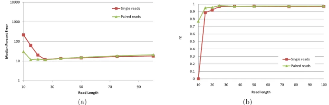
Although high-throughput technologies allow users to make tradeoffs between read length and the number of generated reads, very little has been done to determine optimal parameters even for common applications such as RNA-Seq. The intuition that longer reads are better certainly holds true for many applications such as de novo genome and transcriptome assembly. Surpris-ingly, [20] found thatshorterreads are better for IE when the total number of sequenced bases (as a rough approximation for sequencing cost) is fixed. Fig-ure 1.3.5 plots IE estimation accuracy for reads of length between 10 and 100 when the total amount of sequence data is kept constant at 750M bases. Our results confirm the finding of [20], although the optimal read length is some-what sensitive to the accuracy measure used and to the availability of pairing information. While 25bp reads minimize MPE regardless of the availability of paired reads, the read length that maximizesr2_{is 25 for paired reads and 50 for}

single reads. Although further experiments are needed to determine how the optimum length depends on the amount of sequence data and transcriptome complexity, our simulations do suggest that for isoform and gene expression analysis, increasing the number of reads may be more useful than increasing read length beyond 50 bases.

Figure 1.3.6(a) shows, for reads of length 75, the effects of paired reads and strand information on estimation accuracy as measured byr2_{. Not surprisingly,}

for a fixed number of reads, paired reads yield better accuracy than single reads. Also not very surprisingly, adding strand information to paired sequencing

(33)

yields no benefits to genome-wide IE accuracy (although it may be helpful, e.g., in identification of novel transcripts). Quite surprisingly, performing strand-specific single read sequencing is actuallydetrimentalto IsoEM IE (and hence GE) accuracy under the simulated scenario, most likely due to the reduction in sampled transcript length.

In practice, many RNA-Seq data sets are generated from transcripts with poly(A) tails, and some of the sequenced fragments will contain parts the poly(A) tails. We have added to IsoEM the option to automatically extend annotated transcripts with a poly(A) tail, thus allowing it to use reads coming from such fragments. Table 1.3.4 shows the accuracy of isoform and gene ex-pression levels inferred by IsoEM using 30M reads of length 25 simulated from transcripts with and without poly(A) tails assuming geometric expression of gene isoforms. The accuracy of IsoEM is practically the same under the two simulation scenarios for paired read data, and decreases only slightly for sin-gle reads simulated taking poly(A) tails into account, likely due to the fact that reads overlapping poly(A) tails are more ambiguous.

As shown in Figure 1.3.6(b), the runtime of IsoEM scales roughly linearly with the number offragments, and is practically insensitive to the type of sequencing data (single or paired reads, directional or non-directional). IsoEM was tested on a Dell PowerEdge R900 server with 4 Six Core E7450Xeon Processors at 2.4Ghz (64 bits) and 128Gb of internal memory. None of the datasets required more than 16GB of memory to complete. It is also true that increasing the

(34)

available memory significantly decreases runtime by keeping the garbage col-lection overhead to a minimum. The runtimes in Figure 1.3.6 were obtained by allowing IsoEM to use up to 32GB of memory, in which case none of the datasets took more than 3 minutes to solve.

1.4 Conclusions

In this chapter we have introduced an expectation-maximization algorithm for isoform frequency estimation assuming a known set of isoforms. Our algorithm, called IsoEM, explicitly models insert size distribution, base quality scores, strand and read pairing information. Experiments on both real and synthetic RNA-Seq datasets generated using two different assumptions on the isoform distribution show that IsoEM consistently outperforms existing algorithms for isoform and gene expression level estimation with respect to a variety of quality metrics.

The open source Java implementation of IsoEM is freely available for download at http://dna.engr.uconn.edu/software/IsoEM/.

(35)

5,000 10,000 15,000 20,000 25,000 N u m b e r o f Is o fo rm s 0 5,000 10,000 15,000 20,000 25,000 10 100 1,000 10,000 100,000 N u m b e r o f Is o fo rm s Isoform Length (a) 10000 100000 1000 10000 100000 r o f G e n e s 10 100 1000 10000 100000 N u m b e r o f G e n e s 1 10 100 1000 10000 100000 N u m b e r o f G e n e s 1 10 100 1000 10000 100000 0 5 10 15 20 25 30 35 40 45 50 55 N u m b e r o f G e n e s NumberofIsoforms 1 10 100 1000 10000 100000 0 5 10 15 20 25 30 35 40 45 50 55 N u m b e r o f G e n e s NumberofIsoforms 1 10 100 1000 10000 100000 0 5 10 15 20 25 30 35 40 45 50 55 N u m b e r o f G e n e s NumberofIsoforms (b)

Figure 1.3.1: Distribution of isoform lengths (a) and gene cluster sizes (b) in the UCSC dataset.

(36)

Isoform Expression Gene Expression

Algorithm Uniform Geometric Algorithm Uniform Geometric Uniq 0.466 0.447 Uniq 0.579 0.586 Rescue 0.693 0.675 Rescue 0.724 0.724 UniqLN 0.856 0.838 GeneEM 0.636 0.637 Cufflinks 0.661 0.618 Cufflinks 0.778 0.757 RSEM 0.919 0.911 RSEM 0.939 0.934 IsoEM 0.971 0.970 IsoEM 0.990 0.982

Table 1.3.1: r2_{for isoform and gene expression levels inferred from 30M reads}

of length 25 from reads simulated assuming uniform, respectively geometric expression of gene isoforms.

(37)

100 70 80 90 100 th re sh o ld Uniq 50 60 70 80 90 100 o rm s o v e r th re sh o ld Uniq Rescue UniqLN Cufflinks 20 30 40 50 60 70 80 90 100 % o f is o fo rm s o v e r th re sh o ld Uniq Rescue UniqLN Cufflinks RSEM IsoEM 0 10 20 30 40 50 60 70 80 90 100 0 0.2 0.4 0.6 0.8 1 % o f is o fo rm s o v e r th re sh o ld Uniq Rescue UniqLN Cufflinks RSEM IsoEM 0 10 20 30 40 50 60 70 80 90 100 0 0.2 0.4 0.6 0.8 1 % o f is o fo rm s o v e r th re sh o ld

Relative error threshold

Uniq Rescue UniqLN Cufflinks RSEM IsoEM 0 10 20 30 40 50 60 70 80 90 100 0 0.2 0.4 0.6 0.8 1 % o f is o fo rm s o v e r th re sh o ld

Relative error threshold

Uniq Rescue UniqLN Cufflinks RSEM IsoEM

(a)

100 70 80 90 100 th re sh o ld Uniq 40 50 60 70 80 90 100 g e n e s o v e r th re sh o ld Uniq Rescue GeneEM C ffli k 20 30 40 50 60 70 80 90 100 % o f g e n e s o v e r th re sh o ld Uniq Rescue GeneEM Cufflinks RSEM 0 10 20 30 40 50 60 70 80 90 100 0 0.2 0.4 0.6 0.8 1 % o f g e n e s o v e r th re sh o ld Uniq Rescue GeneEM Cufflinks RSEM IsoEM 0 10 20 30 40 50 60 70 80 90 100 0 0.2 0.4 0.6 0.8 1 % o f g e n e s o v e r th re sh o ld

Relativeerrorthreshold

Uniq Rescue GeneEM Cufflinks RSEM IsoEM 0 10 20 30 40 50 60 70 80 90 100 0 0.2 0.4 0.6 0.8 1 % o f g e n e s o v e r th re sh o ld

Relativeerrorthreshold

Uniq Rescue GeneEM Cufflinks RSEM IsoEM

(b)

Figure 1.3.2: Error fraction at different thresholds for isoform (a) and gene (b) expression levels inferred from 30M reads of length 25 simulated assuming geometric isoform expression.

(38)

Expression range 0 (0,10−6] (10−6,10−5] (10−5,10−4] (10−4,10−3] (10−3,10−2] All # isoforms 13,290 10,024 23,882 18,359 1,182 66 66,803 Uniq 0.0 100.0 98.4 97.1 98.5 96.6 95.4 Rescue 0.0 294.7 75.5 49.2 30.4 28.3 71.9 MPE UniqLN 0.0 100.0 80.8 30.3 26.4 24.8 36.0 Cufflinks 0.0 100.0 49.7 25.5 27.2 44.6 34.1 RSEM 0.0 100.0 31.9 13.5 11.4 13.0 21.2 IsoEM 0.0 100.0 25.3 7.3 3.2 2.2 12.0 Uniq 0.2 98.4 97.2 96.9 97.0 95.5 78.0 Rescue 48.4 95.5 86.2 73.1 61.5 56.1 76.0 EF.15 UniqLN 0.2 97.2 86.2 82.8 83.3 77.3 69.8 Cufflinks 17.6 96.4 81.3 71.0 74.7 80.3 67.9 RSEM 19.9 93.7 71.1 46.4 39.8 47.0 56.9 IsoEM 3.4 93.1 65.1 29.1 11.1 7.6 46.1

Table 1.3.2: Median percent error (MPE) and 15% error fraction (EF.15) for

isoform expression levels inferred from 30M reads of length 25 simulated as-suming geometric isoform expression.

Expression range (0,10−6_{] (10}−6_,₁₀−5_{] (10}−5_,₁₀−4_{] (10}−4_,₁₀−3_{] (10}−3_,₁₀−2_] _All

# genes 120 5,610 11,907 1,632 102 19,372 Uniq 37.4 43.6 42.7 43.0 48.2 43.0 Rescue 32.8 28.7 26.0 25.1 28.8 26.7 MPE GeneEM 30.6 28.2 25.7 25.1 28.0 26.3 Cufflinks 33.0 21.1 19.0 20.2 40.2 19.7 RSEM 23.6 11.0 7.2 7.9 11.4 8.1 IsoEM 18.2 8.4 3.2 2.0 1.9 3.9 Uniq 77.5 82.4 81.7 79.7 82.4 81.7 Rescue 74.2 74.0 71.6 72.8 76.5 72.4 EF.15 GeneEM 72.5 73.8 71.5 73.0 74.5 72.3 Cufflinks 73.3 64.7 62.3 66.2 82.3 63.5 RSEM 64.2 37.3 17.4 16.3 41.2 23.5 IsoEM 57.5 28.1 6.7 6.1 4.9 13.2

Table 1.3.3: Median percent error (MPE) and 15% error fraction (EF.15) for gene

expression levels inferred from 30M reads of length 25 simulated assuming geometric isoform expression.

(39)

R² = 0.4771 100 1,000 C u ff li n k s E st im a te R² = 0.4771 10 100 1,000 10 100 1,000 10,000 C u ff li n k s E st im a te qPCR Estimate (a) R² = 0.5281 100 1,000 Is o E M E st im a te R² = 0.5281 10 100 1,000 10 100 1,000 10,000 Is o E M E st im a te qPCR Estimate (b)

Figure 1.3.3: Comparison of Cufflinks (a) and IsoEM (b) estimates to qPCR expression levels reported in [26].

R² = 0.1158 10.0 100.0 1,000.0 10,000.0 C u ff li n k s E st im a te R² = 0.1158 0.1 1.0 10.0 100.0 1,000.0 10,000.0 0.1 1.0 10.0 100.0 1,000.0 10,000.0 C u ff li n k s E st im a te qPCR Estimate (a) R² = 0.3715 10.0 100.0 1,000.0 10,000.0 100,000.0 Is o E M E st im a te _{R² = 0.3715} 0.1 1.0 10.0 100.0 1,000.0 10,000.0 100,000.0 0.1 1.0 10.0 100.0 1,000.0 10,000.0 Is o E M E st im a te qPCR Estimate (b)

Figure 1.3.4: Comparison of Cufflinks (a) and IsoEM (b) estimates to qPCR expression levels reported in [6].

100 1000 10000 M e d ia n P e rc e n t E rr o r Single reads Paired reads 1 10 100 1000 10000 10 30 50 70 90 M e d ia n P e rc e n t E rr o r Read Length Single reads Paired reads (a) 0.3 0.4 0.5 0.6 0.7 0.8 0.9 1 r2 Singlereads 0 0.1 0.2 0.3 0.4 0.5 0.6 0.7 0.8 0.9 1 10 20 30 40 50 60 70 80 90 100 r2 Read length Singlereads Pairedreads (b)

Figure 1.3.5: IsoEM MPE (a) and r2 _{values (b) for 750Mb of simulated data}

generated using single and paired-end reads of length varying between 10 and 100.

(40)

Reads Poly(A) Isoform Expression Gene Expression 1×25 Yes 0.956 0.977

No 0.970 0.982 2×25 Yes 0.972 0.990 No 0.976 0.985

Table 1.3.4:r2_{for isoform and gene expression levels inferred from 30M single,}

respectively paired reads of length 25, simulated assuming geometric expres-sion of gene isoforms with and without poly(A) tails.

0 955 0.96 0.965 0.97 0.975 0.98 r2 RandomStrandPairs CodingStrand pairs 0.945 0.95 0.955 0.96 0.965 0.97 0.975 0.98 0 10 20 30 40 50 60 r2 MillionReads RandomStrandPairs CodingStrandpairs RandomStrandSingle CodingStrandsingle (a) 60 80 100 120 140 160 C PU se c. RandomStrandPairs CodingStrandPairs RandomStrandSingle CodingStrandSingle 0 20 40 60 80 100 120 140 160 0 10 20 30 C PU se c. MillionFragments RandomStrandPairs CodingStrandPairs RandomStrandSingle CodingStrandSingle (b)

Figure 1.3.6: IsoEMr2_{(a) and CPU time (b) for 1-60 million single}_/_{paired reads}

(41)

Chapter 2 Accurate Estimation of Gene Expression Levels

from DGE Sequencing Data

2.1 Introduction

Massively parallel transcriptome sequencing is quickly replacing microarrays as the technology of choice for performing gene expression profiling due to its wider dynamic range and digital quantitation capabilities. However, accu-rate estimation of expression levels from sequencing data remains challenging due to the short read length delivered by current sequencing technologies and still poorly understood protocol- and technology-specific biases. To date, two main transcriptome sequencing protocols have been proposed in the lit-erature. The most commonly used one, referred to as RNA-Seq, generates short (single or paired) sequencing tags from the ends of randomly generated cDNA fragments. An alternative protocol, referred to as 3’-tag Digital Gene Expression (DGE), or high-throughput sequencing based Serial Analysis of Gene Expression (SAGE-Seq), generates single cDNA tags using an assay in-cluding as main steps transcript capture and cDNA synthesis using oligo(dT) beads, cDNA cleavage with an anchoring restriction enzyme, and release of

(42)

cDNA tags using a tagging restriction enzyme whose recognition site is ligated upstream of the recognition site of the anchoring enzyme.

While computational methods for accurate inference of gene (and isoform) specific expression levels from RNA-Seq data have attracted much attention recently (see, e.g., [1, 20, 32]), analysis of DGE data still relies on direct esti-mates obtained from counts of uniquely mapped DGE tags [35, 40]. In part this is due to salient features of the DGE protocol, which, unlike RNA-Seq, guarantees that each mRNA molecule in the sample generates at most one tag and obviates the need for length normalization. Nevertheless, ignoring ambiguous DGE tags (which, due to the severely restricted tag length, can represent a sizeable fraction of the total) is at best discarding useful informa-tion, and at worst may result in systematic inference biases. In this chapter we seek to address this shortcoming of existing methods for DGE data analysis. Our main contribution is a rigorous statistical model of DGE data and a novel expectation-maximization algorithm for inference of gene and isoform expres-sion levels from DGE tags. Unlike previous methods, our algorithm, referred to as DGE-EM, takes into account alternative splicing isoforms and tags that map at multiple locations in the genome, and corrects for incomplete digestion and sequencing errors. Experimental results show that DGE-EM outperforms methods based on unique tag counting on a multi-library DGE dataset con-sisting of 20bp tags generated from two commercially available reference RNA samples that have been well-characterized by quantitative real time PCR as

(43)

part of the MicroArray Quality Control Consortium (MAQC).

We also take advantage of the availability of RNA-Seq data generated from the same MAQC samples to directly compare estimation performance of the two transcriptome sequencing protocols. While RNA-Seq is clearly more powerful than DGE at detecting alternative splicing and novel transcripts such as fused genes, previous studies have suggested that for gene expression profiling DGE may yield accuracy comparable to that of RNA-Seq at a fraction of the cost [38]. We find that the two protocols achieve similar cost-normalized accuracy on the MAQC samples when using state-of-the-art estimation methods. However, the current protocol versions are unlikely to be optimal. Indeed, the results of a comprehensive simulation study assessing the effect of various experi-mental parameters suggest that further improvements in DGE accuracy could be achieved by using anchoring enzymes with degenerate recognition sites and using partial digest of cDNA with the anchoring enzyme during library preparation.

2.2 DGE Protocol

The DGE protocol generates short cDNA tags from a mRNA population in several steps (Figure 2.1.1). First, PolyA+mRNA is captured from total RNA using oligo-dT magnetic beads and used as template for cDNA synthesis. The double stranded cDNA is then digested with a first restriction enzyme, called

(44)

en-Cleave with anchoring enzyme (AE)

Attach primer for tagging enzyme (TE)

Cleave with tagging enzyme

AAAAA

CATG

AE

TCCRACCATGCATG AAAAA AE

TE

CATG

Map tags

A B C D E

Figure 2.1.1: Schematic representation of the DGE protocol

zyme cleaves cDNA at sites at which the four nucleotide motif CATG appears). We refer to the cDNA sites cleaved by the anchoring enzyme asAE sites. The recognition site of a second restriction enzyme, called Tagging Enzyme (TE) is ligated to the fragments of cDNA that remain attached to the beads after cleavage with the AE, immediately upstream of the AE site. The cDNA frag-ments are then digested with TE, which cleaves several bases away from its recognition site. This results in very short cDNA tags (10 to 26 bases long, de-pending on the TE used), which are then sequenced using any of the available high-throughout technologies.

Since the recognition site of AE is only 4 bases long, most transcripts contain multiple AE sites. Under perfect experimental conditions, full digest by AE would ensure that DGE tags are generated only from the most 3′ _{AE site of}

(45)

1 2 k … 3’ 5’ AE site MRNA Tag formation probability p p(1-p) p(1-p)k-1

Figure 2.2.1: Tag formation probability: pfor the rightmost AE site, geometri-cally decreasing for subsequent sites

sites, or no tag at all. As in [40], we assume that the cleavage probability of the AE, denoted byp, is the same for all AE sites of all transcripts. Since only the most 3′ _{cleaved AE site of a transcript releases a DGE tag, the probability}

of generating a tag from sitei = 1, . . . ,kfollows a geometric distribution with ratio 1−pas shown in Figure 2.2.1, where sites are numbered starting from the 3′end. Note that splicing isoforms of a gene are likely to share many AE sites. However, the probability of generating a tag from a site isisoform specificsince it depends on the number downstream AE sites on each isoform. Thus, although the primary motivation for this work is inference of gene expression levels from DGE tags, the algorithm presented in next section must take into account alternative splicing isoforms to properly allocate ambiguous tags among AE sites.

2.3 DGE-EM Algorithm

Previous studies have either discarded ambiguous DGE tags (e.g. [35, 40]) or used simple heuristic redistribution schemes for rescuing some of them. For example, in [39] the rightmost site in each transcript is identified as a “best” site. If a tag matches several locations, but only one of them is a best site, then

(46)

the tag is assigned to that site. If a tag matches multiple locations, none of which is a best site, the tag is equally split between these locations. In this section we detail an Expectation Maximization algorithm, referred to as DGE-EM, that probabilistically assigns DGE tags to candidate AE sites in different genes, different isoforms of the same gene, as well as different sites within the same isoform.

In a pprocessing step, a weight is assigned to each (DGE tag, AE site) pair, re-flecting the conditional probability of the tag given the site that releases it. This probability is computed from base quality scores assuming that sequencing errors at different tag positions arise independently of one another. Formally, the weight for the alignment of tagtwith the jth_{rightmost AE site in isoform}

i is wt,i,j ∝ Q|_kt₌₁| [(1−εk)Mtk +

εk

3(1−Mtk)], where Mt,k is 1 if position k of tag

t matches the corresponding position at site j in the transcript, 0 otherwise, while εk denotes the error probability of the k-th base of t, derived from the

corresponding Phred quality score reported by the sequencing machine. In practice we only compute these weights for sites at which a tag can be mapped with a small (user selected) number of mismatches, and assume that remaining weights are 0. To each tagtwe associate a “tag class”yt which consists of the

set of triples (i, j,w) whereiis an isoform, jis an AE site in isoformi, andw>0 is the weight associated as above to tagtand site jin isoformi. The collection of tag classes, y=(yt)t, represents the observed DGE data.

(47)

frequencies of each isoform, θ = (fi)i=1,...,m. Let ni,j denote the (unknown)

number of tags generated from AE sitejof isoformi. Thus,x=(ni,j)i,jrepresents

the complete data. Denoting by ki the number of AE sites in isoform i, by

Ni =

Pk_i

j=1ni,j the total number of tags from isoform i, and by N =

Pm

i=1Ni the

total number of tags overall, we can write the complete data likelihood as

g(x|θ)∝ m Y i=1 ki Y j=1 " fi(1−p)j−1p S #ni,j (2.3.1) where S = Pm i=1 Pki j=1 fi(1− p) j−1_p ₌ Pm i=1 fi

1−(1−p)ki_{. Put into words, the}

probability of observing a tag from site jin isoform i is the frequency of that isoform (fi) times the probability of not cutting at any of the first j−1 sites

and cutting at the jth_[(1₋_p₎j−1_p_{]. Notice that the algorithm e}_ff_ectively

down-weights the matching AE sites far from the 3′_{end based on the site probabilities}

shown in Figure 2.2.1. Since for each transcript there is a probability that no tag is actually generated, for the above formula to use proper probabilities we have to normalize by the sumSover all observable AE sites.

Taking logarithms in (2.3.1) gives the complete data log-likelihood:

logg(x|_θ)= m X i=1 ki X j=1

ni,jlog fi+(j−1) log (1−p)+logp−logS+constant

= m X i=1 ki X j=1 ni,jlog fi+(j−1) log(1−p) +Nlogp−Nlog       m X i=1 fi 1−(1−p)ki       +constant

(48)

2.3.1 E-Step

Let ci,j = {yt|∃w s.t. (i, j,w) ∈ yt} be the collection of all tag classes that are

compatible with AE site j in isoform i. The expected number of tags from each cleavage site of each isoform, given the observed data and the current parameter estimatesθ(r), can be computed as

n(_i_,r_j) :=E(ni,j|y, θ(r))= X yt∈ci,j,(i,j,w)∈yt fi(1−p)j−1pw P (l,q,z)∈yt fl(1−p) q−1_pz (2.3.1)

This means that each tag class is fractionally assigned to the compatible isoform AE sites based on the frequency of the isoform, the probability of cutting at the cleavage sites where the tag matches, and the confidence that the tag comes from each location.

2.3.2 M-Step

In this step we want to selectθthat maximizes the Q function,

Q(θ|_θ(r))=Ehlogg(x|_θ)|y, θ(r)i = m X i=1 ki X j=1 n(_ir_,_j) log fi+(j−1) log(1−p) +Nlogp−Nlog       m X i=1 fi 1−(1−p)ki       +constant