Event generator tuning using Bayesian optimization

(1)

Preprint typeset in JINST style - HYPER VERSION

Event generator tuning using Bayesian optimization

Philip Ilten, Mike Williams, and Yunjie Yang

Laboratory for Nuclear Science, Massachusetts Institute of Technology, Cambridge, MA 02139

ABSTRACT: Monte Carlo event generators contain a large number of parameters that must be

determined by comparing the output of the generator with experimental data. Generating enough events with a fixed set of parameter values to enable making such a comparison is extremely CPU intensive, which prohibits performing a simple brute-force grid-based tuning of the parameters. Bayesian optimization is a powerful method designed for such black-box tuning applications. In this article, we show that Monte Carlo event generator parameters can be accurately obtained using Bayesian optimization and minimal expert-level physics knowledge. A tune of the PYTHIA8 event

generator usinge+e− events, where 20 parameters are optimized, can be run on a modern laptop in just two days. Combining the Bayesian optimization approach with expert knowledge should enable producing better tunes in the future, by making it faster and easier to study discrepancies between Monte Carlo and experimental data.

(2)

Contents

1. Introduction 1

2. Bayesian Optimization 2

3. Tuning PYTHIA 3

3.1 Objective Function 3

3.2 Parameters & Observables 4

3.3 Tuning Closure Test 5

3.4 Possible Improvements 7

3.5 Tuning Discrete Parameters 15

4. CPU Usage 15

5. Towards a Real-World Tune 17

6. Summary 18

A. Parameter Uncertainties 19

B. Parameter Results 19

C. Tuning Procedure 20

1. Introduction

Monte Carlo event generators, which are used to simulate particle collisions, contain a large num-ber of parameters that must be determined (tuned) by comparing the output of the generator with experimental data. Generating enough events with a fixed set of parameter values to enable making such a comparison is extremely CPU intensive. For example, it takesO(hour)on a modern CPU core to generate 1M events for a single set of parameter values using the PYTHIA8 event

genera-tor [1, 2]. A full tune of PYTHIAtoe+e−data involves optimizing≈20 parameters, which clearly cannot be performed using a brute-force grid-based approach. Even a tune of only a small subset of parameters,e.g., the 6 parameters that control fragmentation, would takeO(100)CPU years using a coarse 10-bins-per-parameter scheme.

All available tunes provided with the PYTHIA 8 package were obtained either: manually, where an expert chose how to vary the parameters based on extensive knowledge and insight, guided by comparing generated and experimental distributions; orparametrically, where the gen-erator response to changes in the parameters was itself parametrized based on a large set of refer-ence generator data sets, which then facilitated optimizing the parameters via minimization of an

(3)

objective function,e.g., aχ2. Of course, this characterization is oversimplified since experts have performed parametric tunes, but it is sufficient to motivate this study. Examples of manual and parametric tunes are described in detail in Refs. [3] and [4], respectively.

Each of these approaches has both merit and limitations. We believe that only a few physi-cists are capable of performing a large-scale manual tune of PYTHIA, and even for such an expert it takes considerable effort. The manual approach does not scale to larger parameter sets, and is not well suited to less-intuitive models or to producing many experiment-specific tunes (or a large number of dedicated tunes in general). That said, the manual approach is less prone to finding anunphysicallocal minimum in the parameter space that happens to provide a decent description of the data distributions being compared to during the tuning process; the expert can intuitively identify such situations. The parametrization approach is easily parallelized, but requires that the generator response — including multi-parameter correlations — is well approximated by the cho-sen parametric function within the parameter hypercube to be explored. Furthermore, the optimal working point must be included in the parameter hypercube, though this can be achieved by first doing a coarse scan of the parameter space.

In this article, we propose treating Monte Carlo event-generator tuning as a black-box opti-mization problem to be addressed using the framework of Bayesian optiopti-mization. We will show that Monte Carlo generator parameters can be accurately obtained using Bayesian optimization and minimal expert-level physics knowledge. Furthermore, a tune of the PYTHIA8 event generator using e+e− data, where 20 parameters are optimized, can be run on a modern laptop in just two days. Combining the Bayesian optimization approach with expert-level knowledge should enable producing better tunes in the future, by making it faster and easier to study discrepancies between Monte Carlo and experimental data. This article is organized as follows: the Bayesian optimiza-tion framework is described in Sec. 2; its applicaoptimiza-tion to a full PYTHIAe+e− tune is presented in Sec. 3; Sec. 4 describes CPU usage; moving towards a real-world tune is discussed in Sec. 5 and a summary is provided in Sec. 6.

2. Bayesian Optimization

For each Monte Carlo data sample produced by the event generator (for a given set of parameters), a number of observable distributions can be constructed and compared between Monte Carlo and experimental data. Such a comparison is done using an objective function,e.g., a two-sample χ2 statistic built from the binned distributions in data and Monte Carlo.1 Since the dependence of the objective function on the parameters is unknown, the strategy employed in Bayesian optimization is to treat theχ2 as a random function over which a prior must be assigned (see,e.g., Ref. [5]). We choose to use the Gaussian process prior, which is a common choice as it permits computing marginals and conditionals in closed form. For an overview of Gaussian processes, see Ref. [6].

Each time a Monte Carlo sample is generated with a different set of parameters, aχ2value is computed comparing the Monte Carlo to the experimental data. From the initial prior and all of the sampledχ2values, a posterior over functions is constructed. The main idea is to use all information available, and not just the local gradient to find the best possibleχ2. Another choice that must be

1_{In practice, a}

pseudo-χ2statistic is typically used, where correlations between the various observable distributions are ignored. Regardless, a smallerχ2is taken to mean a better tune.

(4)

made in Bayesian optimization is the so-called acquisition function, which is used to determine the next point in parameter space to query. We choose to focus on maximizing the expected improve-ment over the current bestχ2found, as implemented in the SPEARMINTsoftware package [7], and

use the default SPEARMINTsettings for balancing exploration versus exploitation. For a detailed discussion of the algorithms implemented in SPEARMINT, see Ref. [8]. N.b., working within the Gaussian process framework is not suited to discrete parameters; however, other automated opti-mization procedures do handle discrete parameters well (see Sec. 3.5). Finally, it is also possible within Bayesian optimization to account for the CPU cost of generating each Monte Carlo data set, and attempt to maximize the expected improvement per unit time [8].

3. Tuning PYTHIA

To demonstrate how to apply Bayesian optimization to Monte Carlo event generator tuning — and to validate its performance — the following closure test is performed:

• a 10M-evente+e−data sample is generated using PYTHIA8 with its default parameter val-ues, collectively referred to as theMonashtune [3];

• various observable distributions are built from the Monash simulated data sample and treated as experimental data;

• a set of 20 parameters in PYTHIAis chosen for tuning;

• a minimal amount of expert knowledge is input on each parameter, as each is allowed to vary freely within a large pre-defined range (of course, the true Monash values are treated as unknown in the tuning);

• and, finally, the Bayesian optimization framework is applied using SPEARMINTto obtain the

20 optimal (tuned) parameter values.

Treating the Monash data sample as experimental data permits validating the performance by com-paring the Monash parameter values to the optimal ones found by SPEARMINT. This treatment ensures that each distribution can be perfectly modeled by PYTHIA. In reality, Monte Carlo event generators often times do not model parts of the experimental data well; therefore, it is important that any tuning method can also handle optimizing imperfect models (see Sec. 5).

3.1 Objective Function

We define our objective function as a pseudo-χ2in a similar way to the one used in producing the Monash tune [3]: χ2≡ nbins

∑

i=1 (Monashi−MCi)2 σ_Monash2 _,_i+σ_MC2 _,_i , (3.1) whereσ denote the statistical uncertainties on the Monash and Monte Carlo values in theith bin. Anyσivalue that corresponds to less than a 1% relative uncertainty is set to be 1%. The choice of

setting a minimum value avoids having a few bins with large occupancies dominating the tuning. In practice, the systematic uncertainties on the experimental distributions implicitly accomplish this.

(5)

3 10 4 10 5 10 aLund 0 0.5 1 1.5 2 bLund 0.2 0.4 0.6 0.8 1 1.2 1.4 1.6 1.8 2

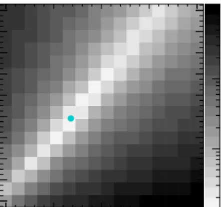
Figure 1.Example of a parameter in PYTHIAthat is not included in our tune. The 10M-event Monash data sample is compared to samples where the aLund and bLund parameters are varied. Thezaxis (greyscale) denotes theχ2value, and the cyan marker shows the Monash value of (aLund, bLund)=(0.68,0.98). The parameters aLund and bLund are strongly correlated, and so only bLund is tuned.

The sample size of each Monte Carlo data set is chosen such that the 1% value is used in most bins. We ignore correlations between bins in our definition of χ2, since this information is often

not available for experimental data. It may be desirable to alter theχ2to include weight factors for

each bin. Incorporating correlations or bin weights into the tuning procedure is straightforward, as only the definition of theχ2needs to be modified.

3.2 Parameters & Observables

Since the Gaussian process framework is not suited to tuning discrete parameters, all discrete pa-rameters in PYTHIAare left at their Monash values.2 We choose to tune a large set of 20 continuous parameters, which roughly corresponds to the full set of PYTHIA8 parameters constrained by the

observable distributions frome+e−data that were used in the Monash tune, and that enter into the

χ2defined in Eq.3.1. This excludes parameters that when varied have either negligible impact on theχ2value, or those that are≈100% correlated with another PYTHIAparameter. An example of a

correlated parameter not included in our tune, aLund, is shown in Fig. 1.N.b., we chose to include in our tune a few parameters that are not well constrained by the χ2 to study how SPEARMINT

performs in the presence of such parameters.

The full list of parameters included in the tune is given in Table 1. The range in which each parameter is allowed to vary is also provided. We place a uniform prior over each parameter within the specified range,i.e., parameters are allowed to vary freely within these ranges. Expert knowl-edge could be used here by assigning non-uniform priors to the parameters that capture the physics belief about their behavior (see Sec. 3.4); however, as our goal in this article is to demonstrate the power of the Bayesian optimization process, we choose to use minimal expert knowledge. For a detailed discussion on the meaning of each parameter, see Ref. [3]. Table 2 provides a full list of

2_{See Sec. 3.5 for discussion on how to tune discrete parameters. We note that no discrete parameters were altered} from the default PYTHIAvalues in the Monash tune itself.

(6)

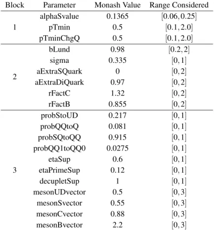
Table 1. Full list of parameters considered in our tune, categorized into blocks, along with their values in the Monash tune and the interval in which we allow them to vary.

Block Parameter Monash Value Range Considered

1 alphaSvalue 0.1365 [0.06,0.25] pTmin 0.5 [0.1,2.0] pTminChgQ 0.5 [0.1,2.0] 2 bLund 0.98 [0.2,2] sigma 0.335 [0,1] aExtraSQuark 0 [0,2] aExtraDiQuark 0.97 [0,2] rFactC 1.32 [0,2] rFactB 0.855 [0,2] 3 probStoUD 0.217 [0,1] probQQtoQ 0.081 [0,1] probSQtoQQ 0.915 [0,1] probQQ1toQQ0 0.0275 [0,1] etaSup 0.6 [0,1] etaPrimeSup 0.12 [0,1] decupletSup 1 [0,1] mesonUDvector 0.5 [0,3] mesonSvector 0.55 [0,3] mesonCvector 0.88 [0,3] mesonBvector 2.2 [0,3]

Table 2. Full list ofe+e−distributions that contribute to theχ2in our tune. The notation “2×” refers to distributions that are considered separately for events with and without abtag.

Category Number Distributions

event shapes 10 2×(thrust,CandDparameter, wide and total jet broadening) fragmentation 6 2×(charged-particle multiplicity and momentum fraction),

scaled momentum spectraxD∗,B≡2pD∗,B/EcmforD∗,Bhadrons

hadron types 4 hadron types ine+e−→XandZ→heavy flavor

the distributions that enter into theχ2defined in Eq.3.1. We choose to use the same set of distri-butions that was used to produce the Monash tune. For our purposes, the physical meaning of each distribution is not important, so we omit any detailed description and instead refer the interested reader to Ref. [3].

3.3 Tuning Closure Test

We consider two approaches to tuning the 20 parameters listed in blocks 1–3 in Table 1 using the χ2built from the 20 distributions given in Table 2:

(7)

• a block-diagonal strategy, where the parameters in blocks 1, 2, and 3 are tuned using only the event-shape, fragmentation, and hadron-type distributions, respectively, and each block is tuned independently;

• and a global strategy, where all 20 parameters are tuned simultaneously on all distributions. The pseudo-experimental data distributions are obtained by generating 10M events using the Monash parameters. For each set of parameters that SPEARMINTchooses to evaluate, a data sample of 1M events is generated. The number of SPEARMINTqueries and the total CPU time used are discussed in Sec.4. In all tunes, the optimal parameter set is taken to be the one that the internal SPEARMINT

χ2model predicts is the best, and not the set for which a PYTHIAdata sample was generated and found to have the bestχ2(in practice this makes little difference). Assigning error bars to parame-ters using the SPEARMINTχ2model is discussed in detail in Appendix A, while more details about the technical aspects of the tuning procedure are given in Appendix C.

Figures 2–4 show the results of tuning the parameters in block 1 on the event-shape distri-butions, while the optimal parameter values are listed in Table 3. The Monash event-shape data distributions are all well described by our tuned PYTHIA spectra. The tuned parameter values are consistent to about ≈1σ based on the uncertainties obtained using the method detailed in Appendix A. The precision on alphaSvalue is 0.0002, while the pTminChgQ confidence interval covers most of the its allowed range. This difference reflects how well the event-shape distributions constrain each parameter.

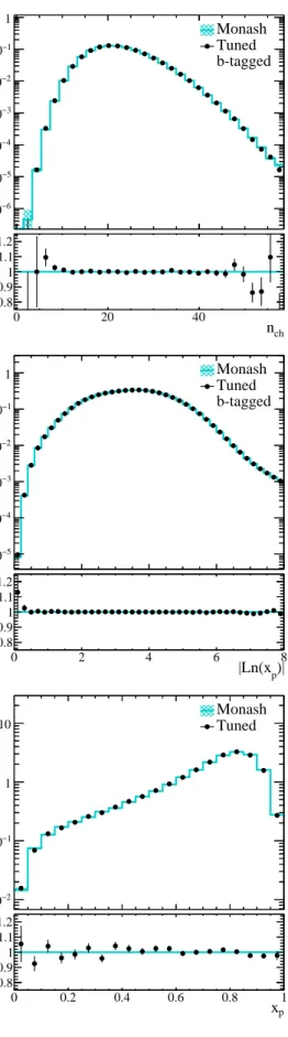
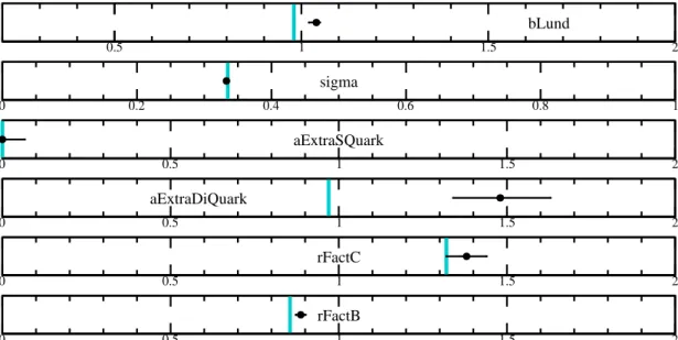
The results of tuning the block 2 parameters on the fragmentation distributions are presented in Figs. 5 and 6, and in Table 4. We again find good agreement between the Monash and tuned spectra. Several of the parameter uncertainties undercover in this case due to sizable correlations,

e.g., the aExtraDiQuark parameter is about 3σ from its Monash value. This parameter is not well constrained by the distributions used and its impact on the χ2 is highly correlated with that of bLund. A proper error bar can be assigned to this parameter by scanning the SPEARMINTmodel in 2-D; however, the simplified uncertainties assigned here, which ignore parameter correlations for the sake of saving CPU, are sufficient to convey how well each parameter is constrained. The parameter aExtraSQuark is only constrained to be.0.1 by the spectra used in the tune, and in such cases we find that SPEARMINTtends to select the edge of the region considered,e.g., aExtraSQuark is tuned to its minimum allowed value of 0.

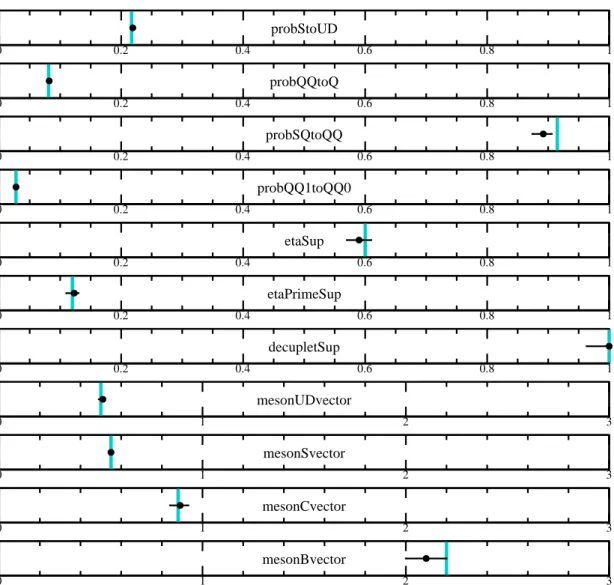
The results of tuning the block 3 parameters on the hadron-type distributions are presented in Figs. 7 and 8, and in Table 5. The block 3 tune involves 11 parameters, and we again find that all data distributions and PYTHIA parameter values are consistent with Monash. Based on these

results, we conclude that SPEARMINThas successfully performed a 20 parameter tune of PYTHIA8 using the block-diagonal strategy that was also employed in the Monash tune [3].

A novel aspect of using the Bayesian optimization framework is the possibility to perform a global tune of all 20 parameters using all 20 distributions — on a laptop. Since most of the 20 parameters considered in oure+e− tune are only strongly constrained by the distributions in a single block, we do not expect a global tune to improve the precision of the tuned parameter values.3 That said, demonstrating that a 20 parameter tune is possible is of interest regardless of

(8)

its utility in this specific example. Figure9 shows the optimal parameter values obtained from the globale+e− tune, compared to those obtained from the tunes of the three blocks. As expected, the global tune does not improve the precision;4however, the fact that such a tune can be run on a laptop is an exciting result. This capability may prove useful in future tunes of Monte Carlo event generators.

The results of our closure test of applying the Bayesian optimization framework to Monte Carlo event generator tuning are summarized as follows:

• The true Monash parameter values are accurately and precisely determined for all parame-ter blocks listed in Table 1, even when a minimal amount of expert knowledge about each parameter is used.

• The three blocks contain 3, 6, and 11 parameters, and no decrease in performance is ob-served in the 11 parameter tune relative to the others. Furthermore, inclusion of a few poorly constrained parameters does not greatly impact the tuning process.

• The uncertainties placed on the tuned parameters using the method described in Appendix A provide reasonable coverage properties in the absence of sizable correlations, and in all cases are sufficient for estimating how well a parameter is constrained by the experimental data distributions.

• A 20 parameter global tune converges to a consistent set of parameter values, except for a few poorly constrained parameters. While the global approach provides no improvement for this particular example, which is expected, the fact that performing a 20 parameter tune is possible is both novel and exciting.

Therefore, this closure test demonstrates that Bayesian optimization is a viable method for tuning Monte Carlo event generators. The real value in its usage for this task will be shown in Sec. 4, where we demonstrate the small CPU required to perform the tunes presented in this section.

3.4 Possible Improvements

An obvious question arises from the study above: is it possible to transfer knowledge gained from the block-diagonal tunes to the global tune? This would permit the global tune to focus on regions of the 20-dimensional parameter space that are known to be promising, rather than simply starting over and ignoring the block-diagonal results. Related applications include transferring knowledge from a tune at one beam energy to another, or from a tune toe+e− data to one on proton-proton data. An interesting area of research on this topic ismulti-taskBayesian optimization [9], which could prove to be useful for tuning Monte Carlo event generators. Another way of potentially speeding up the tuning process would be to first consider theχ2obtained using a smaller generated sample, and then decide whether or not to generate the 1M-event sample based on theχ2value [9].

precision for the parameter due to the increased sample-to-sample variation in the globalχ2 compared to that of the individual blockχ2values.

4_{The uncertainties are underestimated for a few of the parameters in the global tune,}_e.g._{, pTminChgQ. This is likely} due to the global tune being terminated before it had fully converged. Since the global tune is only presented here to demonstrate proof of principle, we have not investigated whether this issue goes away with additional queries.

(9)

d(1-Thrust) σ d σ 1 4 − 10 3 − 10 2 − 10 1 − 10 1 10 2 10 Monash Tuned 1-Thrust 0 0.1 0.2 0.3 0.4 Tuned / Monash 0.8 0.9 1 1.1 1.2 d(1-Thrust) σ d σ 1 2 − 10 1 − 10 1 10 2 10 Monash Tuned b-tagged 1-Thrust 0 0.1 0.2 0.3 0.4 Tuned / Monash 0.8 0.9 1 1.1 1.2 dC σ d _σ 1 2 − 10 1 − 10 1 10 Monash Tuned C 0 0.2 0.4 0.6 0.8 1 Tuned / Monash 0.8 0.9 1 1.1 1.2 dC σ d _σ 1 2 − 10 1 − 10 1 10 Monash_Tuned b-tagged C 0 0.2 0.4 0.6 0.8 1 Tuned / Monash 0.8 0.9 1 1.1 1.2 dD σ d _σ 1 2 − 10 1 − 10 1 10 2 10 _Monash Tuned D 0 0.2 0.4 0.6 0.8 Tuned / Monash 0.8 0.9 1 1.1 1.2 dD σ d _σ 1 2 − 10 1 − 10 1 10 2 10 _Monash Tuned b-tagged D 0 0.2 0.4 0.6 0.8 Tuned / Monash 0.8 0.9 1 1.1 1.2

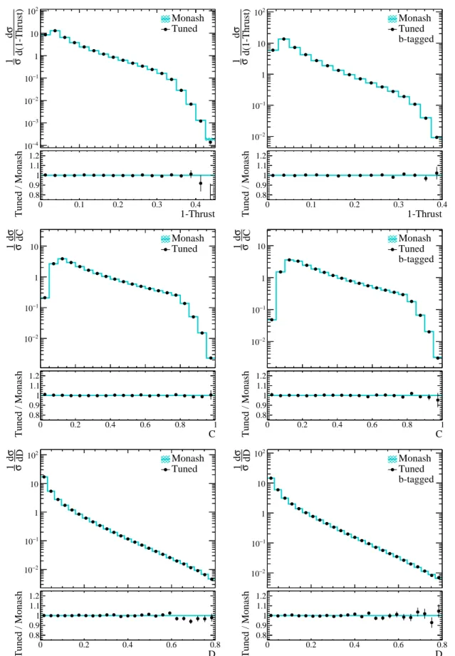
Figure 2.Event-shape distributions obtained from the Monash data sample compared to those obtained from our optimal tune of the parameters in block 1. Both samples used here have 10M events.

(10)

W dB σ d σ 1 3 − 10 2 − 10 1 − 10 1 10 2 10 Monash Tuned W B 0 0.1 0.2 0.3 Tuned / Monash 0.8 0.9 1 1.1 1.2 W dB σ d σ 1 4 − 10 3 − 10 2 − 10 1 − 10 1 10 2 10 Monash Tuned b-tagged W B 0 0.1 0.2 0.3 Tuned / Monash 0.8 0.9 1 1.1 1.2 T dB σ d σ 1 3 − 10 2 − 10 1 − 10 1 10 Monash Tuned T B 0 0.1 0.2 0.3 0.4 Tuned / Monash 0.8 0.9 1 1.1 1.2 T dB σ d σ 1 3 − 10 2 − 10 1 − 10 1 10 2 10 Monash Tuned b-tagged T B 0 0.1 0.2 0.3 0.4 Tuned / Monash 0.8 0.9 1 1.1 1.2

Figure 3. Additional event-shape distributions obtained from the Monash data sample compared to those obtained from our optimal tune of the parameters in block 1. Both samples used here have 10M events.

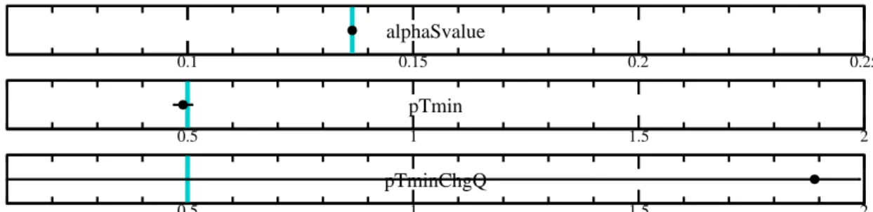
0.1 0.15 0.2 0.25 alphaSvalue 0.5 1 1.5 2 pTmin 0.5 1 1.5 2 pTminChgQ

Figure 4. (black points) Block 1 parameters from our optimal tune compared to their (vertical cyan lines) Monash values. The horizontal-axis ranges are the regions considered by SPEARMINTduring tuning.

(11)

) ch Probability(n 7 − 10 6 − 10 5 − 10 4 − 10 3 − 10 2 − 10 1 − 10 1 Monash Tuned ch n 0 20 40 Tuned / Monash 0.8 0.9 1 1.1 1.2 ) ch Probability(n 6 − 10 5 − 10 4 − 10 3 − 10 2 − 10 1 − 10 1 Monash Tuned b-tagged ch n 0 20 40 Tuned / Monash 0.8 0.9 1 1.1 1.2 )|_p /d|Ln(x ch > dn ch 1/<n 3 − 10 2 − 10 1 − 10 1 Monash_Tuned )| p |Ln(x 0 2 4 6 8 Tuned / Monash 0.8 0.9 1 1.1 1.2 )|_p /d|Ln(x ch > dn ch 1/<n 5 − 10 4 − 10 3 − 10 2 − 10 1 − 10 1 Monash Tuned b-tagged )| p |Ln(x 0 2 4 6 8 Tuned / Monash 0.8 0.9 1 1.1 1.2 p /dx D > dn D 1/<n 2 − 10 1 − 10 1 10 Monash Tuned p x 0 0.2 0.4 0.6 0.8 1 Tuned / Monash 0.8 0.9 1 1.1 1.2 p /dx_B > dn B 1/<n 2 − 10 1 − 10 1 10 Monash Tuned p x 0 0.2 0.4 0.6 0.8 1 Tuned / Monash 0.8 0.9 1 1.1 1.2

Figure 5. Fragmentation distributions obtained from the Monash data sample compared to those obtained from our optimal tune of the parameters in block 2. Both samples used here have 10M events.

(12)

0.5 1 1.5 2 bLund 0 0.2 0.4 0.6 0.8 1 sigma 0 0.5 1 1.5 2 aExtraSQuark 0 0.5 1 1.5 2 aExtraDiQuark 0 0.5 1 1.5 2 rFactC 0 0.5 1 1.5 2 rFactB

(13)

> ch <n <n> 2 − 10 1 − 10 1 Monash Tuned ± π _π0 _K± η η' ρ± _ρ0 *± K ω φ * /K-K R Rφ/K*Rφ/K-Rφ/π -Tuned / Monash 0.8 0.9 1 1.1 1.2 > ch <n <n> 4 − 10 3 − 10 2 − 10 1 − 10 1 Monash Tuned p Λ RΛ/p RΛ/K _Σ± _Σ0 _∆++ _Σ* _Ξ± _Ξ*0 _Ω Tuned / Monash 0.8 0.9 1 1.1 1.2 X) → <n> or BR(Z 3 − 10 2 − 10 1 − 10 1 Monash Tuned ± D _D0 *± D D±s Λ+cX g→ cc J/ψ χc1 ψ3685 Tuned / Monash 0.8 0.9 1 1.1 1.2 X) → <n> or BR(Z 4 − 10 3 − 10 2 − 10 1 − 10 1 Monash Tuned X + B _B± 0 * uds B 0X s B BbqqX g→ bb bbbb+X Υ(× 10) Tuned / Monash 0.8 0.9 1 1.1 1.2

Figure 7. Hadron-type distributions obtained from the Monash data sample compared to those obtained from our optimal tune of the parameters in block 3. Both samples used here have 10M events.

(14)

0 0.2 0.4 0.6 0.8 1 probStoUD 0 0.2 0.4 0.6 0.8 1 probQQtoQ 0 0.2 0.4 0.6 0.8 1 probSQtoQQ 0 0.2 0.4 0.6 0.8 1 probQQ1toQQ0 0 0.2 0.4 0.6 0.8 1 etaSup 0 0.2 0.4 0.6 0.8 1 etaPrimeSup 0 0.2 0.4 0.6 0.8 1 decupletSup 0 1 2 3 mesonUDvector 0 1 2 3 mesonSvector 0 1 2 3 mesonCvector 0 1 2 3 mesonBvector

(15)

0.1 0.15 0.2 0.25 alphaSvalue 0.5 1 1.5 2 pTmin 0.5 1 1.5 2 pTminChgQ 0.5 1 1.5 2 bLund 0 0.2 0.4 0.6 0.8 1 sigma 0 0.5 1 1.5 2 aExtraSQuark 0 0.5 1 1.5 2 aExtraDiQuark 0 0.5 1 1.5 2 rFactC 0 0.5 1 1.5 2 rFactB 0 0.2 0.4 0.6 0.8 1 probStoUD 0 0.2 0.4 0.6 0.8 1 probQQtoQ 0 0.2 0.4 0.6 0.8 1 probSQtoQQ 0 0.2 0.4 0.6 0.8 1 probQQ1toQQ0 0 0.2 0.4 0.6 0.8 1 etaSup 0 0.2 0.4 0.6 0.8 1 etaPrimeSup 0 0.2 0.4 0.6 0.8 1 decupletSup 0 1 2 3 mesonUDvector 0 1 2 3 mesonSvector 0 1 2 3 mesonCvector 0 1 2 3 mesonBvector

Figure 9.(red points) Global tune of the block 1, 2, and 3 parameters compared to their (vertical cyan lines) Monash values. The horizontal-axis ranges are the regions considered by SPEARMINTduring tuning. (black points) The block-diagonal results for each parameter are also shown.

(16)

3.5 Tuning Discrete Parameters

As noted above, the Gaussian process framework is not suited for tuning discrete parameters; how-ever, other automated optimization procedures do handle discrete parameters well. For example, tree-based optimizers handle both discrete and continuous parameters naturally. Such optimizers are available in open-source packages, e.g., the SCIKIT-OPTIMIZE package [10]. To study this, we perform a modified tune of block 1 using SCIKIT-OPTIMIZE, where the under-constrained pa-rameter pTminChgQ is left fixed to its Monash value, and the discrete papa-rameter MEcorrections is added to the tuning process.5 MEcorrections is a binary parameter in PYTHIAthat turns on or off matrix-element corrections in the parton shower. Within about 20 queries, SCIKIT-OPTIMIZE

chooses MEcorrections to be on (the same as its Monash setting), while also tuning alphaSvalue and pTmin to within about 10% of their Monash values. This is an encouraging result, and demon-strates the potential to automatically tune discrete parameters; however, we find that the precision achieved on the continuous parameters is worse when using a tree-based optimizer, which is not surprising given that the tree-based approach does not try and model the dependence of theχ2 on the parameters. There is also no obvious way of assigning uncertainties to the continuous param-eters using this approach that itself does not require substantial CPU resources. Therefore, some combination of tree-based and Gaussian-process-based optimization may be desirable, if discrete parameters are also to be tuned. The tree-based approach can be used first to fix any discrete pa-rameters, and to determine a smaller region to explore for each continuous parameter. Next, the Gaussian process framework can be employed to precisely determine the continuous parameters, and assign uncertainties to them.

4. CPU Usage

The CPU cost of performing these tunes depends on how many queries are made by SPEARMINT;

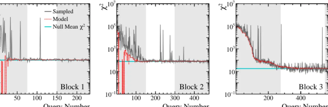
therefore, determining when to terminate the optimization process governs how much total CPU is required. Figure 10 presents the evolution of the SPEARMINTmodelχ2value versus query number for each tuning block. In each case, the SPEARMINTmodel χ2 converges to a value close to the mean χ2 value under the null hypothesis (see Appendix A for details on how the mean value is obtained);i.e., the SPEARMINTmodelχ2 converges to the meanχ2value expected using the true parameter values. Therefore, by first computing the null meanχ2using a Monte Carlo data sample constructed to have per-bin errors that match the experimental data distributions — where the true parameters are known — it is possible to obtain an estimate of what the SPEARMINTmodel χ2 value should converge to.

Figure 10 shows that for each tuning block considered in our study, the SPEARMINTmodelχ2 value is unstable until about 25·n(par)queries are made, and that each block has fully stabilized by 50·n(par)queries (n(par)denotes the number of parameters being tuned). Figures 12-14 show how the optimal SPEARMINT model parameter values evolve with the number of queries. The optimal parameter values also begin to stabilize around 25·n(par)queries, and are found to vary

5_Technically, _{MEcorrections here refers to two P}_YTHIA _parameters: _{TimeShower:MEcorrections and}

SpaceShower:MEcorrections. In this tune, we turn both of them either on or off, so effectively there is one binary parameter.

(17)

by negligible amounts relative to their uncertainties beyond 50·n(par)queries. All tuning results shown in the previous section are obtained using 50·n(par)queries. Based on the results of the tunes performed in this study, some possible stopping criteria are:

• the number of queries reaching a maximum value,e.g., 50·n(par)for the case where each parameter is allowed to vary freely within a large region (less queries are required if smaller regions are explored, see below);

• comparing the SPEARMINTmodelχ2 value after each query to the expected null mean χ2

value, and terminating the tuning process when these values converge,e.g., if they differ by less than a fewχ2units;

• terminating once the stability of the SPEARMINTmodel χ2 over the previous≈5·n(par)

queries is better than a fewχ2units.

Applying any of these criteria to our tunes results in stopping after roughly the same number of queries, with negligible differences in the tuned parameter values. N.b., it is possible to restart a tune in SPEARMINTafter it has been terminated, even if the termination was executed via a SIGINT call,e.g., CTRL-c.

The wall time required to perform these tunes on a quad-core i7 2.8 GHz 2015 Macbook Pro laptop are about 6, 14, and 25 hours for blocks 1, 2, and 3, respectively.6 The CPU per parameter increases roughly linearly going from 3 to 11 parameters. In total, 45 hours of wall time is required to perform the full 20 parameter block-diagonale+e−tune; therefore, a fulle+e− tune of 20 PYTHIA parameters can be performed on a laptop in less than 2 days using SPEARMINT. The event-generation processes dominate the total CPU required to tune each block. Since event generation is trivial to do in parallel, the tunes of each block could be performed much faster using more computing power.

Bayesian optimization implementations like SPEARMINTare not designed for the case where

n(par)10 parameters; however, as shown above, a global tune of all 20e+e−parameters does converge to a consistent set of optimal parameter values, and it does so using the same total number of queries,i.e.our global tune was also terminated after 50·n(par)queries. Despite this, the global tune takes about 3 times more wall time to run because SPEARMINTuses more CPU to determine the next set of parameters to query when there are 20 parameters rather than when there are.11. This results in a sizable increase in the wall time required to perform the global tune because

SPEARMINT runs on a single core. For n(par)≈20, this likely could be sufficiently mitigated

by parallelizing SPEARMINT to permit running on a few cores. To use Bayesian optimization to perform a tune with a much larger number of parameters, changes to the algorithm are likely required (see,e.g., Ref. [11]).

Finally, we note that a much smaller number of queries is required to reach convergence if the parameters are restricted to localized regions around their true values. For example, restricting each well-constrained parameter to vary within a±10σ region around its Monash value, whereσ denotes the quoted uncertainty on each parameter in our block-diagonal tunes, results in all three

6_{This laptop has 8 virtual cores. We run S}_PEARMINT_{on one core, and P}_YTHIA_{event generation is performed in} parallel on the remaining 7 cores.

(18)

Query Number 50 100 150 200 2 χ 1 − 10 10 3 10 5 10 7 10 Sampled Model 2 χ Null Mean Block 1 Query Number 100 200 300 400 2 χ 1 − 10 10 3 10 5 10 7 10 Block 2 Query Number 200 400 2 χ 1 − 10 10 3 10 5 10 7 10 Block 3

Figure 10. Theχ2value for each SPEARMINTquery obtained using (black) the PYTHIAsample produced for the current query and (red) the SPEARMINT χ2model. The white regions show 25·n(par)–50·n(par) queries for each block.

tuning blocks converging in .10·n(par) queries. This is similar to the number of queries re-quired by parametric tuning methods [4], where such restricted regions must be used to ensure that the generator response is well approximated by a low-order parametric function. Which approach should be employed in a real-world tune depends on what knowledge exists about the parameters. If it is known that the optimal parameter values must be within a small region, and that within this region the generator response is well approximated by a low-order parametric function, then the parametric approach is likely the best option. Conversely, if little is known about the opti-mal parameter values, then Bayesian optimization would be preferable. One could also consider employing SPEARMINTto determine the parameter values used by a subsequent parametric tune.

5. Towards a Real-World Tune

There are a number of issues that arise in a real-world tune (see,e.g., Refs. [12, 13, 14]) that are absent from the closure test presented above; however, our view is that each of these factorizes from the process of efficiently exploring the parameter space.

• The goal of the tuning closure test presented above was to demonstrate the power of the Bayesian optimization method; therefore, we chose to use minimal expert knowledge by placing a uniform prior over each parameter within a large specified range. In a real-word tune, expert knowledge could be used here by assigning non-uniform priors to the parameters that capture the physics belief about their behavior, which could include expected correla-tions between parameters.

• In a real-world tune, it may be desirable to weight the various bin contributions in the χ2 definition, rather than treating them all equally as we did. This is trivial to implement as it only requires changing theχ2value reported to the optimizer.

• Our tuning closure test only involvede+e−collisions at a single energy, whereas many real-world tuning applications involve several beam types at multiple energies. From the perspec-tive of the optimizer, this situation is no different than the simple case of one beam type and

(19)

energy. The optimizer provides the set of parameter values for the next query, then waits to receive theχ2value; it does not need to know how theχ2is obtained. We presented the CPU

requirements in the previous section in terms of the number of queries because this is more universally applicable than CPU time;i.e.the CPU per query depends greatly on the beam types and energies to be generated, but in all cases the approach that minimizes the number of queries should also require the least CPU resources.

• In a real-world tune, even once the optimal parameter values are found, one expects discrep-ancies between the Monte Carlo and data will remain. Discovering such situations as quickly as possible should be viewed as one of the goals of the parameter-optimization process. As an example, rather than treating the Monte Carlo generated using PYTHIAand the Monash pa-rameters as experimental data, we performed a tune of block 1 using actual experimental data [15]. The tune converges in about the same number of queries as in the closure test, and theχ2value ob-tained is almost two times better thanχ2obtained using the Monash parameter values. While this result demonstrates successful application of the optimization process to experimental data, some care is needed to interpret this result. Since Monash is meant to be a global tune of PYTHIA, the selection of the block 1 parameters includes expert-level physics knowledge beyond the input dis-tributions used to construct theχ2. Such knowledge could be included in the Bayesian optimization process by placing non-uniform priors over the parameters. Alternatively, since a model of param-eter dependence of the χ2 is built during the tuning process, the expert could choose to perform various block-specific tunes first using uniform priors. Next, the expert could study how eachχ2 value depends on the parameters and choose how to combine these results using their knowledge to obtain the optimal result — or to decide where to improve the Monte Carlo generator. Regard-less, by combining the Bayesian optimization approach with expert-level knowledge, it should be possible to produce better tunes in the future by making it much faster and easier to both optimize the generator parameters and to study discrepancies between Monte Carlo and experimental data.

6. Summary

Monte Carlo event generators contain a large number of parameters that must be determined by comparing the output of the generator with experimental data. Generating enough events with a fixed set of parameter values to enable making such a comparison is extremely CPU intensive. All available tunes provided with the PYTHIA 8 package were obtained either manually or

para-metrically. In this article, we proposed to instead treat Monte Carlo event generator tuning as a black-box optimization problem and addressed it using the framework of Bayesian optimization. We showed that Monte Carlo generator parameters can be accurately obtained using Bayesian op-timization and minimal expert-level physics knowledge. Using this approach, a tune of PYTHIA8 usinge+e− data, where 20 parameters were optimized, was run on a laptop in just two days. Fi-nally, we believe that combining the Bayesian optimization approach with expert-level knowledge should enable producing better tunes in the future, by making it faster and easier to study discrep-ancies between Monte Carlo and experimental data. The code used in this study is available at Ref. [16].

(20)

2 χ 50 100 150 200 units 2_χ Fraction / 5 0.00 0.01 0.02 0.03 Block 1 2 χ 0 50 100 150 units 2_χ Fraction / 5 0.00 0.01 0.02 0.03 Block 2 2 χ 0 20 40 60 80 100 units 2_χ Fraction / 5 0.00 0.02 0.04 Block 3

Figure 11. χ2distributions for each tuning block obtained using the true (Monash) parameter values. The vertical lines show (dashed black) the meanχ2value and (solid red) the final SPEARMINTmodel of theχ2 value.

Acknowledgments

This work was supported by DOE grants DE-SC0010497 and DE-FG02-94ER40818. We thank A. Buckley, T. Head, G. Louppe, and T. Sjöstrand for useful discussions and feedback.

A. Parameter Uncertainties

The SPEARMINTmodel of how the objective function depends on the parameters is conceptually different than a χ2 statistic obtained from a single two-sample test; therefore, we cannot simply use∆χ2=1, or similar criteria, to estimate the uncertainty on the parameters. Figure11 shows the distribution ofχ2values obtained from an ensemble of two-sample tests in each parameter block under the null hypothesis. These distributions are obtained by performing a large number of two-sample comparisons using theχ2 in Eq. 3.1, where all samples are generated using the Monash parameters, one sample contains 1M events, and the other 10M events. Figure 11 shows that the

SPEARMINTmodel accurately predicts the mean value of eachχ2distribution.

As anad hocmethod for assigning uncertainties to tuning parameters, we scan the SPEARMINT

modelχ2value while varying each parameter independently and holding all other parameters fixed to their tuned values (often referred to as the plugin method). The 1σ confidence interval for each parameter is taken to include all parameter values for which the SPEARMINTmodelχ2is less than χ2(p=0.32), whereχ2(p=0.32)is theχ2value corresponding to ap-value of 0.32 for the case where the number of degrees of freedom equals the mean χ2value predicted by the SPEARMINT

model. While this approach is certainlyad hoc, it produces confidence intervals with reasonable coverage properties in each of the tunes presented above, and at minimal CPU cost.

B. Parameter Results

The tuning results for each parameter for the three blocks are given in Tables 3–5. The evolution of the parameter values during the tuning processes are shown in Figs. 12–14.

(21)

Table 3.Tuning results for block 1.

Parameter Monash Value Tune Value Range Considered

alphaSvalue 0.1365 0.1365±0.0002 [0.06,0.25]

pTmin 0.5 0.49±0.02 [0.1,2.0]

pTminChgQ 0.5 1.89₋+0₁_..10₇₉ [0.1,2.0]

sigma 0.335 0.333₋+0₀._.001₀₀₂ [0,1] bLund 0.98 1.04₋+₀0._.01₀₂ [0.2,2] aExtraSQuark 0 0+₋0₀.07 [0,2] aExtraDiQuark 0.97 1.48₋+0₀._.15₁₄ [0,2] rFactC 1.32 1.38±0.06 [0,2] rFactB 0.855 0.887±0.015 [0,2]

probStoUD 0.217 0.219₋+0₀._.001₀₀₂ [0,1] probQQtoQ 0.081 0.082±0.01 [0,1] probSQtoQQ 0.915 0.892₋+0₀._.014₀₁₈ [0,1] probQQ1toQQ0 0.0275 0.0276±0.0009 [0,1] etaSup 0.6 0.59±0.02 [0,1] etaPrimeSup 0.12 0.12±0.01 [0,1] decupletSup 1 1+₋0₀_.₀₄ [0,1] mesonUDvector 0.5 0.51₋+0₀._.01₀₂ [0,3] mesonSvector 0.55 0.55±0.01 [0,3] mesonCvector 0.88 0.89₋+0₀._.04₀₅ [0,3] mesonBvector 2.2 2.1±0.1 [0,3] C. Tuning Procedure

In this section, we provide more details regarding the technical aspects of the tuning procedure. All of the code required to reproduce the studies presented in this work is available at the GitHub repos-itory TUNEMC [16], and fully documented there (including installation and usage instructions).

Schematically, the tuning proceeds as follows:

• a large (10M-event)e+e−data sample is generated using PYTHIA8 with its default param-eter values, collectively referred to as theMonashtune [3], and various observable distri-butions are built from the Monash simulated data sample and treated as experimental data (in a real-world tuning application, this step would be replaced by the use of experimental

(22)

distributions);

• a set of parameters in PYTHIAis chosen for tuning (we chose to tune 20 parameters), and for each parameter a range of values to consider is defined;

• for each query, the Bayesian optimization package SPEARMINTprovides a set of parameter values which are passed to PYTHIA 8 and used to generate 1M events (we chose to use a

fixed number of events per sample though, as discussed in the text, one could consider using a variable number [9] which may improve the CPU usage);

• once the PYTHIAsample is generated for each parameter set, the observable distributions are

constructed and used to calculate the objective function value according to Eq. 3.1, which is provided to SPEARMINTand used to update its internal model from which the next set of parameters to query is determined and passed to PYTHIA;

• the query steps are repeated until some chosen stopping criterion (see Sec. 4) is met.

N.b., by default SPEARMINTprovides the suggested parameter sets in series, though it is possible

for these to be provided in parallel. However, since the CPU usage is dominated by PYTHIAevent generation—and because we performed this study on a small number of CPU cores—we chose to parallelize the event-generation processes for each sample, rather than generate multiple samples in parallel. Specifically, we split up the generation of each 1M-event sample into multiple jobs run in parallel, but ran SPEARMINTin series mode. For a larger-scale tuning application, it may also

be advantageous to parallelize the queries. References

[1] PYTHIAhome page: http://home.thep.lu.se/Pythia/.

[2] T. Sjöstrandet al., Comput. Phys. Commun.191, 159 (2015), 1410.3012. [3] P. Skands, S. Carrazza, and J. Rojo, Eur. Phys. J.C74, 3024 (2014), 1404.5630.

[4] A. Buckley, H. Hoeth, H. Lacker, H. Schulz, and J. E. von Seggern, Eur. Phys. J.C65, 331 (2010), 0907.2973.

[5] J. Mockus, Bayesian Approach to Global Optimization: Theory and Applications(Kluwer Academic Publishers, 1989).

[6] C. E. Rasmussen and C. K. I. Williams,Gaussian Processes for Machine Learning(MIT Press, 2006). [7] SPEARMINTGitHub repository: https://github.com/HIPS/Spearmint.

[8] J. Snoek, H. Larochelle, and R. P. Adams, Practical bayesian optimization of machine learning algorithms, inAdvances in Neural Information Processing Systems 25, edited by F. Pereira, C. J. C. Burges, L. Bottou, and K. Q. Weinberger, pp. 2951–2959, Curran Associates, Inc., 2012.

[9] K. Swersky, J. Snoek, and R. P. Adams, Multi-task bayesian optimization, inAdvances in Neural Information Processing Systems 26, edited by C. J. C. Burges, L. Bottou, M. Welling, Z. Ghahramani, and K. Q. Weinberger, pp. 2004–2012, Curran Associates, Inc., 2013.

(23)

[11] K. Kandasamy, J. Schneider, and B. Poczos, High dimensional bayesian optimisation and bandits via additive models, inProceedings of The 32nd International Conference on Machine Learning 2015, 2015.

[12] ATLAS, (2012), ATL-PHYS-PUB-2012-003, ATL-COM-PHYS-2012-738. [13] CMS, V. Khachatryanet al., Eur. Phys. J.C76, 155 (2016), 1512.00815.

[14] LHCb, I. Belyaevet al., Handling of the generation of primary events in Gauss, the LHCb simulation framework, inProceedings, 2010 IEEE Nuclear Science Symposium and Medical Imaging

Conference (NSS/MIC 2010): Knoxville, Tennessee, October 30-November 6, 2010, pp. 1155–1161, 2010.

[15] L3, P. Achardet al., Phys. Rept.399, 71 (2004), hep-ex/0406049. [16] TUNEMC GitHub repository: https://github.com/yunjie-yang/TuneMC.

(24)

Query Number 50 100 150 200 alphaSvalue 0.1 0.15 0.2 0.25 Sampled Model Monash Query Number 50 100 150 200 pTmin 0.5 1 1.5 2 Query Number 50 100 150 200 pTminChgQ 0.5 1 1.5 2

Figure 12. Evolution of the parameter values in block 1 during the tuning process. The white regions are 25·n(par)–50·n(par)queries.

Query Number 100 200 300 400 bLund 0.5 1 1.5 2 Query Number 100 200 300 400 sigma 0 0.2 0.4 0.6 0.8 1 Query Number 100 200 300 400 aExtraSQuark 0 0.5 1 1.5 2 Query Number 100 200 300 400 aExtraDiquark 0 0.5 1 1.5 2 Query Number 100 200 300 400 rFactC 0 0.5 1 1.5 2 Query Number 100 200 300 400 rFactB 0 0.5 1 1.5 2

(25)

Query Number 200 400 probStoUD 0 0.2 0.4 0.6 0.8 1 Query Number 200 400 probQQtoQ 0 0.2 0.4 0.6 0.8 1 Query Number 200 400 probSQtoQQ 0 0.2 0.4 0.6 0.8 1 Query Number 200 400 probQQ1toQQ0 0 0.2 0.4 0.6 0.8 1 Query Number 200 400 etaSup 0 0.2 0.4 0.6 0.8 1 Query Number 200 400 etaPrimeSup 0 0.2 0.4 0.6 0.8 1 Query Number 200 400 decupletSup 0 0.2 0.4 0.6 0.8 1 Query Number 200 400 mesonUDvector 0 1 2 3 Query Number 200 400 mesonSvector 0 1 2 3 Query Number 200 400 mesonCvector 0 1 2 3 Query Number 200 400 mesonBvector 0 1 2 3