A microsimulation analysis of the mobility impacts of intersection ramp metering

(1)

Copyright by

William Jared Wall 2013

(2)

The Thesis Committee for William Jared Wall

Certifies that this is the approved version of the following thesis:

A Microsimulation Analysis of the Mobility Impacts of Intersection

Ramp Metering

APPROVED BY

SUPERVISING COMMITTEE:

C. Michael Walton Jing (Peter) Jin

(3)

A Microsimulation Analysis of the Mobility Impacts of Intersection

Ramp Metering

by

William Jared Wall, B.S.Civ.Eng.

Thesis

Presented to the Faculty of the Graduate School of The University of Texas at Austin

in Partial Fulfillment of the Requirements

for the Degree of

Master of Science in Engineering

The University of Texas at Austin

December 2013

(4)

Dedication

To my amazing wife Lauren-Leigh, whose love, support, patience, and sacrifice have made all of this possible.

(5)

v

Acknowledgements

I would like to acknowledge Dr. Peter Jin, not only for developing the initial concept of Intersection Ramp Metering, but also for his assistance and guidance throughout this thesis.

(6)

vi

Abstract

A Microsimulation Analysis of the Mobility Impacts of Intersection

Ramp Metering

William Jared Wall, M.S.E. The University of Texas at Austin, 2013

Supervisor: C. Michael Walton

Urban freeway demand that frequently exceeds capacity has caused many agencies to consider many options to reduce congestion. A series of solutions that falls under the Active Traffic Management (ATM) banner have shown promising potential. Perhaps the most popular ATM strategy is ramp metering. Ramp metering involves limiting the access of vehicles to freeways at an entrance ramp. By doing this, freeway throughput, speeds, and travel time reliability can be increased, while the number of traffic incidents can be decreased. This study examines the application of an innovative ramp metering strategy, Intersection Ramp Metering (IRM), at a section of Loop 1 in Austin, TX. IRM implements the ramp metering function at the intersection immediately upstream of the entrance ramp, rather than on the ramp itself. A microsimulation analysis of this application is performed in VISSIM, and the results confirm that freeway throughput (+10%), and system average travel time (-14%), can be improved, as well as several other performance measures.

(7)

vii

List of Tables

Table 2.1: Popular ATM Technologies ...6

Table 2.2: Required Distance between Meter and Freeway Merge Point ...26

Table 2.3: Appropriate Travel Times Between Intersections ...34

Table 6.1: Initial VAP Parameter Settings ...57

Table 6.2: Optimal VAP Parameter Settings – Scenario 1 ...59

Table 6.3: Optimal VAP Parameter Settings – Scenario 2 ...61

Table 6.4: System-wide Results ...69

Table 6.5: Freeway and Arterial Performance Results ...71

Table 6.6: Travel Time Reliability Results ...73

Table 6.7: System-wide Impacts of Queue Flushing ...74

(10)

x

List of Figures

Figure 2.1: Ramp Meter Geometric Characteristics ...9

Figure 2.2: Required Detector Locations for ALINEA ...13

Figure 2.3: Comparison between Feed-Forward and Feedback Control ...14

Figure 2.4: Required Detector Locations for Demand Capacity and Occupancy Control ...15

Figure 2.5: Detector Requirements for ZONE and Stratified Ramp Metering ...21

Figure 2.6: Variation in Queue Discharge Rate During Phase Interval in Saturated Conditions ...27

Figure 2.7: Approximate Relationship between Delay and Cycle Length ...29

Figure 2.8: Texas Three-Phase Control Strategy ...32

Figure 2.9: Texas Four-Phase Control Strategy ...33

Figure 2.10: NEMA Phase Numbering ...33

Figure 3.1: Intersection System Design and Phase Plan ...36

Figure 5.1: Analysis Area ...46

Figure 5.2: Data Collection Equipment ...47

Figure 5.3: Aerial of Data Collection Location ...47

Figure 5.4: View of Intersection 1 ...48

Figure 5.5: View of Intersection 2 ...48

Figure 5.6: View From Bridge ...49

Figure 5.7: Measured Volumes ...50

Figure 5.8: Observed Traffic Flows ...51

Figure 5.9: Observed Interchange Timings ...52

(11)

xi

Figure 6.2: Interchange Timings for Scenario 2 ...61

Figure 6.3: Queue Clearance Detector Placement ...62

Figure 6.4: Measured Avergage Freeway Flows for Base Case and Scenario X 64 Figure 6.5: Measured Average Freeway Flows and Speeds for Scenario 1 ...65

Figure 6.6: Measured Average Freeway Flows and Speeds for Scenario 2 ...66

Figure 6.7: Measured Average Freeway Flows and Speeds for Scenario 3 ...67

Figure 7.1: Example Frontage Road Intersection Metering Layout ...79

Figure 7.2: Gap Control Sign ...81

(12)

1

Chapter 1: Introduction

Urban freeways are becoming increasingly congested during peak hours. Many

of these facilities are approaching or have already reached capacity. Particularly, the

travel periods during the morning and afternoon peak hours see significant congestion.

Agencies all across the country have been exploring many different options to ease this

congestion. There are only three basic ways congestion can be lessened: increasing

capacity, improving system operations, or reducing demand. Historically, the solution to

congestion has been to increase capacity. This led to the construction and expansion of

the freeway system that we currently have. However, demand has been constantly

increasing and many of these expansions merely keep congestion at constant levels.

Many cities across the country have expanded their freeways near the absolute limit, yet

congestion is still increasing. Now that system expansion is becoming an increasingly

difficult option, transportation officials must now look to improving operations and

reducing demand as the primary approach toward easing this congestion.

One heavily researched and tried and true method of improving operations is

Active Traffic Management (ATM). Many agencies are now turning to various ATM

strategies to help alleviate congestion and improve system performance. ATM involves

the implementation of intelligent transportation systems to dynamically manage traffic

operations based on prevailing conditions to alter traffic flow and driver behavior [1]. It

can be helpful toward alleviating both recurrent and non-recurrent congestion. Typically

applied toward urban freeways, most ATM strategies can delay the onset of or reduce the

(13)

2

objectives of such systems is to improve travel time reliability. An additional windfall for

many ATM strategies is that they concurrently increase system throughput and improve

highway safety by reducing the number and severity of crashes.

The travel time reliability of a roadway segment is dictated by the amount and

character of congestion that that particular stretch of road experiences. The indices that

describe travel time reliability are measures of the variation in travel times across a

segment for different users. The higher this variation, the less reliable that segment will

be for producing consistent travel times.

The designed goal of many ATM strategies is to improve flow along a freeway,

either by implementing a control system on the mainlines or at a freeway entrance ramp.

One of the more commonly used ATM strategies implemented at entrance ramps is ramp

metering. Ramp metering involves controlling the access of vehicles entering a segment

of freeway. With only a traffic control signal, entrance ramp flows can be easily adjusted

by the presiding agency. By carefully adjusting the rate at which vehicles can enter the

freeway, several operational benefits can be obtained.

At uncontrolled ramps, random vehicle arrivals and large platoons arriving from

surface street intersections complicate merging and weaving movements and cause a

traffic breakdown that has the potential to propagate upstream. These locations are

considered bottlenecks for the mainlines of a freeway. By guaranteeing a uniform arrival

rate and breaking up these vehicle platoons, ramp metering will mitigate or in some cases

even eliminate the traffic breakdown that occurs at these points [2]. This uniform arrival

(14)

3

system is properly calibrated, it has the potential to increase freeway volumes, increase

overall travel speeds, reduce incident rates, and decrease fuel consumption and vehicular

emissions [3].

The first ramp metering system was implemented on the Eisenhower Expressway

in Chicago, Illinois in 1963. It consisted of a traffic officer standing on the ramp and sending vehicles to the freeway one at a time at a predetermined rate. By the 1970’s,

cities such as Minneapolis, Minnesota began using permanent traffic control devices.

These early devises were pre-timed with fixed metering rates [4]. The 1990’s saw a rise

in the use of traffic responsive systems, which yielded much better system performance

results. Today, more sophisticated ramp metering systems are being widely used in at

least 29 cities in the United States [5].

Austin, Texas suffers from some of the worst freeway congestion in the nation,

according to researchers at the Texas Transportation Institute. They estimate that Austin

commuters spend an average of 44 hours a year stuck in traffic. These delays add up to

an annual cost of $930 per commuter. Austin has the worst planning time index score in

the state, at 4.26. This means that for a trip that would take 30 minutes under

uncongested conditions, commuters should allow themselves 2 hours and 8 minutes to be

assured to making to their destination in time. Austin’s planning time index score was

the 6th worst of the 101 largest U.S. cities included in the study. It is apparent that an

(15)

4 1.1 – Problem Statement

In this research, a novel ramp metering approach is introduced. It seeks to

facilitate the ramp metering process at the intersection immediately upstream of the

entrance ramp, as opposed to the ramp itself. This process is called Intersection Ramp

Metering (IRM). This method will have limited applicability, specifically to where ramp

geometries do not allow for a traditional ramp metering system, and where there is plenty

of queue storage at the intersection approach. This technique could be further beneficial,

in that it could reduce the cost associated with having to install a separate traffic control

hardware system on the ramp. Instead, it uses the existing hardware at the intersection.

The additional cost could be eliminated altogether if the intersection controller is

sophisticated enough to facilitate a ramp metering algorithm and could be connected to

detectors on the freeway mainlines, if these detectors already exist. However, if detectors

need to be installed, this would not be cost incurred over traditional ramp metering

systems because mainline detectors are needed for each. Like traditional ramp metering

systems, this system strives to improve travel conditions on the freeway by carefully

controlling the dispatch of vehicles onto the freeway.

In addition to the description of the system is an initial evaluation of its

effectiveness. It is important to remember that the freeway and performance effects of

IRM are not intended to be superior to existing ramp metering techniques; instead it is

intended to be equally as effective as the existing systems. The evaluations consist of

(16)

5

using real peak hour traffic data collected from that site. Several different evaluation

scenarios are presented, and recommendations are made regarding the results.

1.2 – Thesis Summary

This thesis introduces and evaluates a novel ramp metering approach where the

control is applied at the immediate upstream intersection instead of the ramp itself.

Chapter 2 summarizes general active traffic management strategies as well as several

ramp metering control algorithms and traffic signal control timing optimization

strategies. Chapter 3 describes the methodology of the research. Chapter 4 presents the

development of the microsimulation model. Chapter 5 discussed the design of the

experiment. Chapter 6 presents the simulation results of the research. Chapter 7

discusses recommendations and conclusions based on these results as well as future

(17)

6

Chapter 2: Literature Review

2.1 Summary of Prevailing ATM Technologies

Active traffic management is defined by the Federal Highway Administration

(FHWA) as the “ability to dynamically manage recurrent and non-recurrent congestion based on prevailing and predicted traffic conditions.” Specifically, its intention is to

improve trip reliability, maximize the effectiveness of a system, and improve safety

through the use of systems integrated with technology. Crucial to the effectiveness of

ATM is that it features the automation of dynamic deployment, rather than deployment

by human operators. Most ATM strategies work by simply influencing driver behavior in

a way that will improve system operations. The most popular ATM strategies are

summarized in Table 2.1 below [1].

Table 2.1 - Popular ATM Technologies

ATM

Strategy Concept

Used on Freeway or Arterial

Control System Traffic Impact Adaptive

Ramp Metering

Traffic Signals on freeway onramps dynamically control the rate of vehicles dispatched from ramp based on mainline freeway conditions

Freeway Traffic Control Signal, Capable Signal Controller, Mainline and Ramp Detectors Improved Freeway flow and travel speeds, reduced delay

(18)

7 Table 2.1 (continued) – Popular ATM Technologies

ATM

Control System Traffic Impact Adaptive

Traffic Signal Control

Continuously monitors arterial traffic conditions and adjusts intersection timing (phase lengths, cycle lengths, offsets, etc.) to achieve predetermined objective (minimize delay, maximize flow, etc.). Often monitors traffic well upstream of intersection so that arriving traffic patterns are known.

Arterial Traffic Control Signal, Capable Signal Controller, traffic detectors at intersection and upstream Increase in throughput, decrease in delay and queue lengths Dynamic Junction Control

Dynamically controls lane assignments at freeway onramps and off-ramps based on prevailing freeway and arterial conditions. For example, when exiting volumes are high relative to through freeway volumes, the right freeway lane could be designated as exit-only. If entering volumes are high relative to existing freeway volumes, a lane drop could be implemented upstream of the entrance ramp to allow

entering vehicles an additional acceleration lane

Freeway Lane Assignment Indicators, detectors on mainlines and ramps and/or arterials Increase in throughput, decrease in delay Dynamic Lane Reversal

Reverses travel direction on lanes to dynamically allocate directional capacities based on prevailing traffic conditions. Freeway or Arterial Lane Assignment Indicators, detectors on mainlines Increase in capacity Dynamic Lane Use Control

Dynamically opens or closes lanes based on existing freeway

conditions. It can be used in advance of recurrent bottlenecks or incidents. Advanced warning is provided to assist merging movements upstream of the lane closure

Freeway Lane Status Indicators

Increase in throughput, decrease in delay

(19)

8 Table 2.1 (continued) – Popular ATM Technologies

ATM

Control System Traffic Impact

Dynamic Merge Control

Dynamically manages the merging of vehicles based on prevailing travel conditions. It can provide guidance and merging instructions well upstream of a merge point

Freeway Merge Control Signage Increase in throughput, decrease in delay Dynamic Shoulder Lanes

Dynamically allows usage of road shoulder to increase the roadway capacity during congested periods. It can be used either during

recurrent bottlenecks or unexpected conditions such as incidents.

Freeway Shoulder Opening Status Signage Increase in capacity Dynamic Speed Limits

Dynamically changes speed limits based on prevailing freeway traffic or weather conditions. Can be freeway wide or individual lane assigned limits,

Freeway Speed Limit Signage and mainline detectors Uniform Speed Queue Warning

Dynamically displays warnings of downstream queues or bottlenecks in an attempt to lessen shockwaves and reduce rear-end crashes

Freeway Queue Warning Signage Uniform Speed Transit Signal Priority

Dynamically adjusts intersection signal timings upon the arrival of a transit bus, by either extending the green interval or bringing up the green interval sooner, in an attempt to lessen the number of intersections the bus will stop at.

Arterials Bus detection sensors, Capable Traffic Controllers

Decrease in transit travel time

(20)

9 2.2 Ramp metering

Ramp metering control is implemented on freeway entrance ramps. While the

control strategies and logic may be unique for different systems, the basic concept is the

same. By installing ramp meters, engineers can control the rate that vehicles are allowed

to enter a freeway, reduce freeway demand, and break up vehicle platooning caused by

releases from upstream signals [2]. Figure 2.1 below shows the basic layout for either a

single lane or dual-lane ramp metering system.

Figure 2.1 - Ramp Meter Geometric Characteristics

It can be seen above that the meter is typically placed on the ramp, where

sufficient acceleration distance for freeway-bound vehicles can be provided. It is also

important that the meter not be located so far up the ramp that there will not be enough

(21)

10

The FHWA, in their Ramp Management and Control Handbook, recommends

agencies consider the following 6 elements before determining their ramp metering

strategy [7]:

 Geographic extent – the ramp metering will either be isolated around one or several ramps, or it will be a part of a larger coordinated system

 Approach – pre-timed or traffic responsive

 Metering algorithm – logic used to determine the metering rate

 Queue management – how ramp queues will be held to an acceptable length  Flow control – how vehicles will be dispatched from the ramp (one at a time or

several at a time)

 Signing – how drivers will know if the system is on or off

Each of these six elements is important in determining how a ramp metering

system will be implemented. However, the importance of each of these can be ranked

differently by different individuals.

Determining whether or not a pre-timed or traffic responsive approach will be

best depends on the type of congestion that is occurring, and the amount of detectors that

are available. In general, the traffic benefits of a traffic responsive system are greater, but

so are the capital costs. If the congestion is predictable and nearly always recurrent, a

pre-timed system may be an acceptable approach. This is particularly true when there are

no detectors on the ramp or on the mainline near the ramp. If the agency determines that

(22)

11

would not be possible. Furthermore, there are two degrees of traffic responsive systems.

One will switch on the metering system when the traffic reaches a critical point. In this

system, the ramp metering will begin at a predetermined rate. Another type of traffic

responsive system, and the one that is used by a majority of modern agencies, is one in

which the ramp metering rate itself is determined by traffic conditions. Typically the

ramp discharge rate will be lower when there is more congestion on the mainline [7].

There are several metering algorithms that are commonly used in practice, and

several more that have been developed but have yet to be implemented. Each algorithm

utilizes a different control logic, and each has different singular objectives. However, the

goal of each is to lessen freeway congestion and improve system performance. In

general, the more complex an algorithm is, the more sophisticated the controller hardware

must be and more detectors that would be required. This would make the system more

susceptible to equipment failures and would make it more expensive [8]. For this reason,

many agencies prefer the simple, yet very well performing, techniques.

There are two different types of ramp metering strategies, local and coordinated.

Coordinated systems will typically use local control algorithms on the ramp level, and include some further control logic that seeks to weave each ramp’s operations together to

achieve optimal operations throughout a freeway corridor. The following are three of the

most popular local control strategies, ALINEA, Demand Capacity, and Occupancy

(23)

12 2.2.1 ALINEA

One of the more common algorithms for ramp metering is called Asservissement LINéaire d’Entrée Autoroutière, or simply, ALINEA. ALINEA is a very popular local

feedback ramp metering strategy. It has been used extensively with little tweaking since

its introduction in the early 1990’s. It is still used widely throughout Europe with much

success [10]. The intent of the ALINEA system is to maximize mainline flow by

maintaining a desired occupancy level. Hence, it only requires one detector per lane,

which will be located downstream of the entrance ramp. Because mainline occupancy is

the only determinate for a standard ALINEA system, no detectors are required on the

entrance ramp itself. The control algorithm for ALINEA calculates metering rates that

will be applied to achieve the desired mainline occupancy. The following equation is

used to calculate the ramp metering rates in ALINEA [11]:

( ) ( ) [ ( )]

Where r(t) is the ramp metering rate at time step t, Odes is the desired occupancy,

which is typically the critical occupancy, where the freeway’s flow is maximized.

Typical values for the desired occupancy range from 18% to 31% [12]. Odn is the

measured downstream occupancy at time t, r(t-1) is the metering rate from the previous time period, and Kr is a regulatory parameter [3]. A value of 70 vehicles per hour has

been used extensively for Kr with much success [13]. One of the key operational advantages of ALINEA is both the simplicity of the control algorithm and the minimal

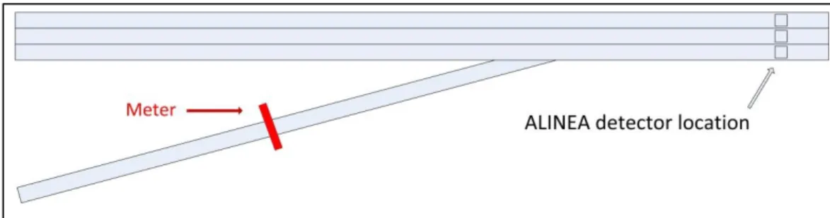
detector requirements. Figure 2.2 depicts the required detector locations for ALINEA.

(24)

13

detector within the determined time-step for this equation to hold true [3]. Oftentimes,

the available detector location will be the key parameter in determining the time-step

length.

Figure 2.2 - Required Detector Locations for ALINEA

The ALINEA technique is a tried and true method that has performed well over

many simulations and field implementations with minimal adjustments. Papageorgiou et

al. lists the many benefits of ALINEA, which includes its simplicity due to only one

control equation and variable, its low implementation cost, its efficiency, and its

flexibility due to the fact that the desired occupancy level can be adjusted at any time,

either automatically or manually.

Furthermore, since ALINEA is a feedback control philosophy, it attempts to avoid

freeway congestion before it occurs, rather than control it after it occurs, which is what is

done in feed-forward control philosophies. By the feedback approach being based on

downstream measurements rather than upstream measurements, it is theoretically more

suitable for controlling downstream conditions than a feed-forward approach, such as

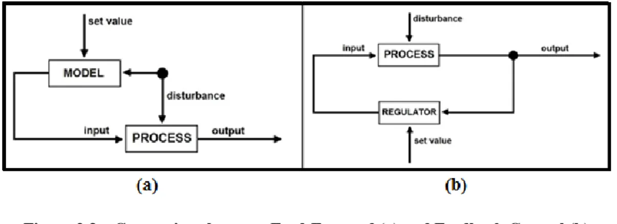
Demand Capacity or Occupancy Control [13]. Consider the following control diagram

(25)

14

Figure 2.3 – Comparison between Feed-Forward (a) and Feedback Control (b)

This control diagram represents the logic of the feed-forward and feedback

approaches. The feed-forward system is regulated by a set value for a parameter; which

in the case for our example is the desired mainline flow. The process output would be

mainline flow, which we desire to be equal to the freeway capacity. The process input

would be the onramp flow, which is dictated by our calculated ramp metering rate. The

disturbance would be the mainline upstream conditions. In order to achieve the desired

output, this type of system measures the disturbances and applies what the model

calculated to be the appropriate input to be combined with the disturbance to achieve the

desired output. For this reason this type of approach is often called disturbance

compensation. Because of the presence of immeasurable disturbances, this structure is

highly sensitive. Furthermore, the success of this system is reliant on a highly accurate

model, because the output is never measured and the model is never readjusted to reach a

more suitable output. A more robust approach is the feedback control approach, which is

utilized by the ALINEA algorithm [11]. This approach is represented by the control

(26)

15

In this approach, the output is considered rather than the disturbance. We still

have our set value acting as the regulator, but in this instance it is modifying the

controllable input to keep the output as close to the desired value as possible. By the

input being consistently readjusted based on the output, we can be certain that we are

producing a stronger result. In the previous feed-forward approach, the output is never

measured; therefore we have to trust the accuracy of our model and the measured

disturbances in order to be assured we are near our desired output. In the feedback

approach, we are updating the input based on the output, and can therefore be certain we

are nearing the desired output assuming only modest changes in the disturbance [13].

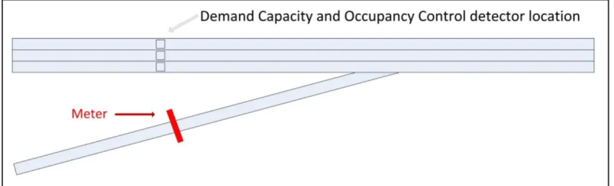
Two popular feed-forward approaches are Demand Capacity and Occupancy

Control [8]. Because these approaches employ a feed-forward approach, the freeway

occupancy is measured upstream of the merge point. The detector locations are shown in

Figure 2.4 below.

(27)

16 2.2.2 Demand Capacity

The Demand Capacity strategy (DC) utilizes the following equation to determine

ramp metering rates:

( ) { ( ) ( )

Where qcap is the capacity of the downstream freeway segment, qup (t – 1) is the

upstream freeway flow at time t-1, Oup (t-1) is the upstream freeway occupancy, Ocr is the

critical downstream occupancy where freeway flow is at its maximum, and rmin is the

minimum allowable ramp flow.

This strategy seeks to add to the upstream flow the amount of ramp flow

necessary to reach the downstream capacity. If the last measured upstream occupancy is

greater than the critical occupancy, the system reverts to sending the lowest allowable

flow [10]. The rmin is a parameter that would be determined by the agency implementing

the system, and would typically be a function of the ramp queue length, storage capacity,

and vehicle arrival rate.

2.2.3 Occupancy Control

Occupancy control (OCC) is a special form of the DC strategy that assumes a

linear relationship between the occupancy and flow at a point on the freeway is

maintained up until the critical occupancy is reached. This relationship can be described

by the following equation:

(28)

17

Where vf is the freeway free-flow speed and g is the g-factor that converts

occupancy to density. This formula yields an estimation of qup based on the measured

occupancy, which can, under certain circumstances, reduce implementation costs [13].

With this estimation having been made, the metering rate is the same rate that is used in

DC when the measured occupancy is under the critical value, which is shown in the

following formula:

( ) ( )

This is a simpler version of the DC strategy, but is even more inaccurate due to

the assumption of linearity from the fundamental diagram [10].

These control algorithms describe how vehicles are dispatched from a single ramp

during the ramp metering process. Papageorgiou et al. argues that ALINEA is superior to

DC and OCC because of the fact that occupancy is the controlled variable, rather than

volume, because traffic volumes over a detector will be the same for congested and light

traffic [13]. Another advantage cited is that the critical occupancy is less sensitive to

weather and outside influences than the capacity is.

When multiple ramps are considered together, a coordinated system may be

developed. Most coordinated systems use one of the above mentioned local ramp

metering algorithms at the individual ramp level. The following describes several

(29)

18 2.2.4 ZONE

The ZONE algorithm was originally used in Minneapolis, Minnesota. This system

divides a freeway segment into various zones, between 3 to 6 miles in length, which are

characterized by boundaries an upstream free-flow section and a downstream bottleneck

section. The objective is to maximize throughput through these bottleneck locations [14].

The algorithm seeks to control volumes within the zone. The control equation is:

( )

Where M is the total volume of the metered ramps in the zone, F is the total metered freeway to freeway ramp volumes, X is the total off-ramp volumes, B is the volumes of the downstream bottleneck section at capacity (usually assumed to be

approximately 2,200 vehicles per hour per lane), S is the space available within the zone,

which is estimated based on mainline occupancy, A is the measured volumes at the upstream free-flow section, and U is the total measured volumes of the non-metered ramps. In this equation, M and F are variables that can be controlled; all others are either

measured or pre-set. For each individual meter, two metering rates are calculated. One is

a local occupancy control algorithm, which is an overriding mechanism intended for

non-recurring congestion. The other is a system-level metering rate that is determined by

comparing the five measured variables (X, B, S, A, and U) with a series of thresholds based partly on historic peak hour traffic volumes [15].

Although the system was continuously amended to improve performance, public

skepticism over the effectiveness of ramp metering began to rise along with the rise in demand throughout the 1990’s. Eventually, it was mandated that for an 8 week period in

(30)

19

2000, the entire Minneapolis ramp meter system would be shut off, and before and after

data compared.

The findings from the mandatory shutdown confirmed that the ZONE metering

system reduced freeway congestion, freeway delays, fuel consumption, vehicular

emissions, and number of incidents. At the same time, it increased freeway throughput

and average speed and it optimized freeway merging [16].

2.2.5 Stratified ZONE

Although the ramp-meter holiday proved the system wide benefits of ramp

metering, there was still some controversy over onramp wait times. This forced the

Minnesota DOT to consider the ramp queues, and a new system was developed for the

region called stratified ramp metering [15]. The stratified ramp metering system still

incorporates the basic concept of ZONE, but it also factors in ramp demand and queue

sizes. The control objectives are listed as:

1. Control flow into a zone so that the capacity is not exceeded

2. Limit ramp wait times to below the predetermined value

In order to achieve these objectives, the system utilizes a hierarchal control

structure with two tiers. The first involves the zone itself. All ramp meters within a zone

are assigned an allocated proportion of zonal capacity, based on their respective ramp

demands. The ramp metering rates are based upon this allocation, provided they are

within the predetermined range of acceptable metering rates, which is determined to be

(31)

20

overlapping zones, the most restrictive metering rate is always used. The release rates

and control logic are very similar to those used by the ZONE system.

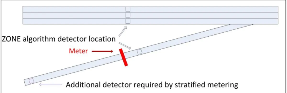
The second tier in the hierarchy involves the ramp itself. Two ramp status

variables are introduced, ramp demand and minimum release rate. Ramp demand is the

hourly flow rate of vehicles wishing to enter a ramp, and is measured by a detector

located at the far upstream end of the ramp and another just past the stop bar of the ramp.

The minimum release rate is time-varying and is calculated from the ramp queue lengths.

This variable is important in ensuring that the ramp wait times are below the

predetermined value. The formula used for calculating the minimum rate is:

Where N is the number of vehicles in the queue and Tmax is the predetermined

maximum allowable ramp wait time for a vehicle, which is 2 minutes for a

freeway-to-freeway ramp and 4 minutes for a standard local access ramp. Because the calculation of

ramp demand requires an upstream ramp detector, stratified ramp metering has a greater

number of detector requirements than ZONE. A schematic depicting the ramp level

(32)

21

Figure 2.5 - Detector Requirements for ZONE and Stratified Ramp Metering

When the proposed release rate determined in the first tier drops below the

minimum release rate determined in the second tier, the minimum release rate overrides

until the proposed rate is once again greater than the minimum. If the override feature is

triggered and is maintained throughout several control cycles, the minimum release rate

will gradually increase until it reaches the ramp flushing rate of 1,714 vehicles per hour.

If this scenario occurs, it will have a negative impact on freeway conditions.

The stratified system has met its objectives of improving ramp wait times, but this

is achieved at the detriment of several mainline performance measures. However, results

have shown that total system performance is still improved over the non-metering case

[15].

Selection of a ramp metering algorithm is an important step in implementing a

ramp metering system. Each agency, upon deciding that they want to use ramp meters,

will need to select the algorithm that best suits their desired objectives, and is best

(33)

22 2.2.6 Queue management

Queue management is an important issue, and one of the main reasons the

Minnesota DOT switched from ZONE to Stratified ZONE as mentioned above. In the

year 2000, Minneapolis performed the famous experiment where the ramp metering

system was shut off for an 8 week period. The catalyst for this experiment was largely

public outrage over the effectiveness of the ramp metering systems, which primarily

stemmed from long onramp wait times. The study ultimately concluded that ramp

metering provided an overall benefit in both safety and mobility to freeway facilities, but

it also highlighted that onramp wait times were often unbearably long during the ramp

metering operation. These conclusions led to the development of the stratified ramp

control algorithm, which factors ramp queues in the calculation of the ramp metering

rate. A successful ramp metering system should never have queues that back up to the

point where they adversely affect surface street traffic. In fact, many systems include

detectors at the far upstream end of an entrance ramp that will turn off the ramp metering

system when it reaches a certain occupancy level. This process is known as ramp

flushing [3].

Ramp flushing policies are usually implemented to ensure that ramp metering

does not adversely affect the performance of surface street intersections. However, much

research suggests that not only does ramp flushing degrade the performance of ramp

metering; it may even cause the system to perform worse than a non-metered ramp

would. Several simulation results have shown that when ramp flushing is permitted, the

(34)

23

ramp demand is greater than the meter capacity for any time period throughout normal

operations, then a ramp meter that permits flushing should not be installed.

2.2.7 Flow control

There are three popular strategies for characterizing the flow of vehicles through a

ramp metering system. The first, and most popular, is a single-lane one car per green

strategy. This approach allows one car to enter the freeway for every ramp metering

cycle. The second approach is a single-lane multiple car per green strategy. This is also

known as platoon or bulk metering. Here, two or more vehicles are allowed to enter the

freeway each metering cycle. This approach is less effective towards improving freeway

conditions, because it essentially recreates small platoons. Also, this approach does not

necessarily increase the capacity of metering systems, because the longer greens times

require longer yellow times. Therefore there are not as many ramp metering cycles,

hence the lack of any significant increase in capacity. Finally, is dual-lane metering.

This consists of two adjacent lanes on the freeway entrance ramp, which reduces to one

lane before the freeway merge. The dispatch pattern for this dual-lane approach allows

the first vehicle in one lane to go, followed by the first vehicle from the next lane.

Because a vehicle from one lane can be released while a vehicle in the other lane is still

coming to a stop at the meter, this approach can sustain about 90% more capacity than a

(35)

24 2.2.8 Signing

Signing for ramp metering systems should be done such that users will be able to

quickly and easily identify how the system works and when it is on. The FHWA’s

Manual on Uniform Traffic Control Devices requires that only 6 standards be followed

when implementing ramp metering systems, which are listed below as shown in Section

4I.02 and 4I.03 [17]:

 Ramp control signals shall meet all of the standard design specifications for traffic control signals, except as otherwise provided in this Section.

 The signal face for freeway entrance ramp control signals shall be either a two-section signal face containing red and green signal indications or a three-two-section signal face containing red, yellow, and green signal indications.

 If only one lane is present on an entrance ramp or if more than one lane is present on an entrance ramp and the ramp control signals are operated such that green signal indications are always displayed simultaneously to all of the lanes on the ramp, then a minimum of two signal faces per ramp shall face entering traffic.  If more than one lane is present on an entrance ramp and the ramp control signals

are operated such that green signal indications are not always displayed simultaneously to all of the lanes on the ramp, then one signal face shall be provided over the approximate center of each separately-controlled lane.

 Ramp control signals shall be located and designed to minimize their viewing by mainline freeway traffic.

 The RAMP METERED WHEN FLASHING sign shall be supplemented with a warning beacon (see Section 4L.03) that flashes when the ramp control signal is in operation.

(36)

25 2.2.9 Geometric Requirements

The installation of a ramp meter signal on an entrance ramp should only be

attempted if the location meets certain geometric requirements. In their Roadway Design

Manual, the Texas Department of Transportation (TxDOT) provides requirements for

minimum ramp length [2].

First, there must be sufficient stopping distance from the upstream intersection to

the back of the queue. This point coincides with location of a queue detector. TxDOT’s

design criteria suggests that for a 35 mph design speed, no less than 240 ft. would be

desired as the stopping distance. This value was calculated using the American

Association of State Highway and Transportation Official’s (AASHTO) stopping sight

distance equation [18].

Additionally, there must be sufficient storage space on the ramp itself for vehicles

queuing to get on the freeway. This storage space is between the queue detector and the

meter itself. For a single lane meter, the required storage distance in feet is:

Where L is the required storage distance in feet, and V is the expected peak-hour demand in vehicles per hour.

Finally, there must also be enough space provided to allow vehicles to accelerate

comfortably from a stop to a safe merging speed by the time they reach the freeway

merge point. The AASHTO values for this distance based on merging speed and ramp

(37)

26 2.3 Signal Timing

When adjustments are being made to existing signal timings, certain

justifications must be made and certain objectives must be targeted. Because driver

behavior is such an integral part of traffic engineering, there is never one correct optimal

approach for timing an intersection. Typically, however, certain principals are always

followed. One, the total number of phases should be minimized. This is to reduce the

total amount of lost time, or the time that no vehicles are being processed through an

intersection. The more often a phase changes, the more clearance intervals there will have

to be, and the more lost time that will be incurred. Additionally, the analyst should

always seek to maximize the amount of movements that can be served per phase, if

possible. The fewer approaches that are stopped at an intersection, the fewer the vehicles

that will be experiencing stopped delay. In general, signal timing approaches are

designed to minimize the amount of control delay inflicted upon drivers. Table 2.2 - Required Distance between Meter and Freeway Merge Point (ft)

Merging Speed (mph) Ramp Grade (%) -3 0 3 37 295 367 492 43 417 518 682 50 591 748 1027 56 814 1060 1529 62 1086 1450 2182

(38)

27 2.3.1 Webster’s Optimal Cycle Length

One of the more popular signal timing approaches was developed by F.V.

Webster in 1958. He sought to create a timing scheme in which average control delays

could be minimized [19]. In this, he developed one of the first widely used, accurate

measures for control delay. His estimates were based on quantifying the lost time caused

by the starting-up of vehicles in a queue, and the slowing of vehicles as the yellow

indication is displayed. These variances in flow contribute to control delay, in addition to

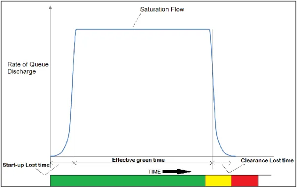
the stopped delay incurred during the red interval. A demonstration of these delays can

be seen in Figure 2.6 below.

Figure 2.6 - Variation in Queue Discharge Rate During Phase Interval in Saturated Conditions

In addition to quantifying the lost times, this approach allows us to quantify the

(39)

28

average delay through theoretical assumptions and computer simulations, which is shown

in the following equation:

( )

[ (_{) ]} ( ) ( )

(₎

Where d is the average delay per vehicle for this particular approach in seconds, C is the cycle length in seconds, g is the effective green time in seconds, x is the degree of saturation (this is the ratio of actual flow to maximum possible flow), and q is the arrival rate in vehicles per second.

The first two terms are purely theoretical. The first term quantifies delay based

on a period of uniform arrivals into the intersection. The second term allows for

stochastic variability during periods where a Poisson arrival pattern and a constant

processing rate through the intersection can be assumed. The final term is empirically

derived from the simulation results. Its inclusion makes the model fit the observed

results. This final term makes up only about 10% of the total delay.

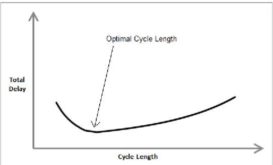
From this equation, a relationship between delay and cycle length can be deduced.

An approximate representation of this relationship is shown in Figure 2.7 below. It can

easily be seen that there is a certain value for cycle length where the total delay is

(40)

29

Figure 2.7 - Approximate Relationship between Delay and Cycle Length

This value for optimal cycle length can be found by differentiating the delay

equation with respect to cycle length and setting it to equal zero. Webster published an

approximated value of this result, citing the true solution as too complicated for practical

applications. Instead, he developed an approximation for optimal cycle length, which is:

∑ ( )

Where Co is the optimal cycle length in seconds, L is the sum of lost time for all phases in seconds (typically assumed to be the sum of all red and yellow intervals), CLVi

is the critical lane volume for approach i, and si is the saturation flow for approach i

(typically 1800 vphpl). The critical lane flow is the flow of the lane with the highest

(41)

30

Once the total cycle length is calculated, phase lengths can be calculated based on

the relative critical lane volumes, as shown in the following equation:

(

∑ ) [( ) (∑( )

)]

Where gi is the green time for phase i, yi is the yellow time for phase i, and ri is the red time for phase i. This relationship basically states that the green time for a cycle should be divided amongst a cycle based on the relative volumes for each phase.

2.3.2 Timing Strategies for Diamond Interchanges

Diamond interchanges present a unique signal timing situation. Because of the

existence of frontage roads, Texas utilizes a slightly different control scheme for diamond

interchanges than other jurisdictions. The phasing plan is dictated by the geometric

allowances of the intersection, which in turn is dictated by the land use pattern adjacent to

the interchange. The key distinction between the different classificational functions of

diamond interchanges is the spacing between the two intersections. These classifications

are as follows:

 Conventional Diamond – Intersection spacing is greater than 800 ft. These interchanges are most commonly found in rural areas and are

typically stop sign controlled.

 Compressed Diamond – Interchange spacing is between 400 and 800 ft. These interchanges are commonly found in suburban areas, and are

(42)

31

typically signal controlled. The two intersections do not have to use an

interconnected signal system.

 Tight Diamond – Interchange spacing is less than 400 ft. These intersections are typically found in urban areas, and will be signal

controlled. Because of the close proximity of the two interchanges, it is

practically required that they be designed as one system.

Researchers at the Texas Transportation Institute summarized guidelines that are

used for timing such intersections in Texas [20]. Basically, for compressed and tight

diamonds, there are two different control strategies that are used, the Texas Three-Phase

and the Texas Four-Phase Control Strategies. The Three-Phase Strategy is best used

when there is sufficient storage between the two intersections, typically a compressed

diamond. This strategy does not seek to ensure that the space between intersections will

be cleared at the end of each phase. A diagram of the Texas Three-Phase Control

(43)

32

Figure 2.8 - Texas Three-Phase Control Strategy

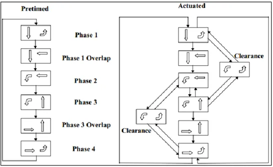
When the intersection spacing is tight and there is little to no storage space in the

area between the two intersections, the phasing pattern should be arranged so that this

space will be cleared at the end of each phase. This is where the Texas Four-Phase

Strategy comes in. It utilizes a split-phasing pattern, with overlaps between frontage road

and arterial phases to prevent excess lost time. The control diagram for this strategy is

(44)

33

Figure 2.9 - Texas Four-Phase Control Strategy

Also, a technique to calculate phase splits is presented. The National Electrical

Manufacturers Association (NEMA) phase numbering system for a diamond interchange

is shown in Figure 2.10 below.

(45)

34

The first step in calculating the phase splits is calculating the overlap. The overlap

calculation is as follows:

Where Φ is the overlap time, ΦLR is the travel time from the left intersection to the

right intersection minus two seconds, and ΦRL is the travel time from the right

intersection to the left intersection minus two seconds. The following table, Table 2.3, is

provided to assist in the determination of travel times between intersections.

Once the overlap time has been determined, and a cycle length has been

pre-determined, the phase splits using the Texas Four-Phase Strategy can be calculated using

the following equation:

( )

Where, ϕi equals the phase time in seconds for phase i,yi is the CLV to saturation flow ratio for phase i, C is the cycle length in seconds, and l is the lost time per phase, in seconds.

Table 2.3 - Appropriate Travel Times Between Intersections Design

Speed (mph)

Link Distance (feet)

100 150 200 250 300 350 400 450 500 550 600 650 700 750 800 20 5 7 9 10 12 14 16 17 19 21 22 24 26 28 29 25 5 7 8 9 11 12 13 15 16 18 19 20 22 23 24 30 5 7 8 9 10 11 13 14 15 16 17 18 19 20 22 35 5 7 8 9 10 11 12 13 14 15 16 17 18 19 20 40 5 7 8 9 10 11 12 13 14 14 15 16 17 18 19 45 5 7 8 9 10 11 12 13 14 14 15 16 17 17 18

(46)

35

Then the odd numbered phases can be calculated as follows:

Once the phase durations have been calculated, the lost time per phase must be

subtracted to get the green time per phase. This approach will give the recommended

(47)

36

Chapter 3: Methodology

3.1 Intersection Ramp Metering System Design

The intent of this research is to design a system that can be implemented with

little to no additional infrastructure requirements. This system would facilitate a

modified ALINEA ramp metering process, using only existing traffic control signals.

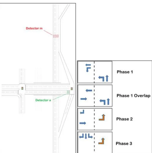
Figure 3.1 below shows the interchange layout as well as the required detector locations

and the existing phasing sequence for the metered intersection, which is the one shown

on the right side of the image.

(48)

37

The interchange analyzed in this research is classified as a tight diamond

interchange, because the intersection spacing is about 340 ft. Due to this classification, it

can be seen above that the intersection is controlled with a modified Texas Four-Phase

Control Strategy. This phasing plan is modified because the arterial does not continue

beyond the right side of the diamond in the above diagram. Because of this, there is no

westbound approach, and no need for what was Phase 2 in the conventional Texas

Four-Phase Strategy.

In this particular application, although the ALINEA algorithm does not require a

detector at the entrance ramp (or in this case Detector a at the intersection approach), the

model code used requires detection of a vehicle for the metering system to be activated.

That is the purpose of Detector a above. The mainline detector, Detector m, is required

for any ALINEA application, and should be located at some point downstream of the

merge point.

The IRM algorithm implements metered control during a particular display in the

phasing sequence. The metered movements are depicted by the orange arrows in Figure

3.1 above. All normal movements are depicted by blue arrows. In this particular situation,

because measured volumes for the northbound through movement were considerably

low, this movement is not metered. However, for similar intersections, this movement

could also be metered if the volumes warrant it. The proposed phasing sequence will

follow the same pattern as the existing sequence, which, shown in the diagram above, is

(49)

38 3.2 The Intersection ALINEA Algorithm

The ALINEA algorithm can be modified to account for multiple signal heads

using the same downstream detector data, and the inclusion of a maximum and minimum

rate. The system is implemented using the following control logic:

( ) {

( ) [ ( )]

Where r1 (t) is the current ramp metering rate, OCCm is the measured occupancy of the downstream detector, r1 (t-1) is the metering rate during the previous interval, Kr is the regulatory parameter which is set at 70 vehicles per hour, OCCm,des is the desired mainline occupancy, and OCCm (t) is the current measured mainline occupancy. The metering rate is further bound by the predetermined maximum and minimum metering

rates.

The signal control logic converts the ramp metering rate into a signal display. It

does this by calculating the red interval and cycle length for each interval. Since the

green interval is fixed in our approach, the cycle length will always be the sum of the

fixed green interval and the calculated red interval. To determine the red time in the ramp

metering cycle, Tr for the ramp metered approach, the control logic utilizes the following equation:

( )

Where n is the number of lanes, C is the cycle length, g is the intersection green time for the metered approach, and TG is the predetermined green time for the IRM signal. This formula dictates the rate at which vehicles are dispatched to the ramp. At the

(50)

39

same time, it could also be set to ensure that queues for the onramp will not back up and

cause an adverse effect on traffic not wishing to access the freeway. If the occupancy of

a detector placed at the point where queues should not stretch beyond is greater than the

determined threshold, it can be assumed that the queues are backing up into the adjacent

intersection. If the queue reaches this length, then the phase 1 metering rate could be

increased to its maximum value, and the traffic is dispatched to the ramp at that rate until

the detector occupancy is measured to be lower than the maximum value. While this process, known as “ramp flushing”, will lessen the effectiveness of our ramp metering

procedure, it is occasionally a necessary element of the system design. It is not feasible

to imagine an implementation of this system where onramp queues that are blocking

other movements will be acceptable. Because of this, the availability of storage space at

the intersection is an important parameter in determining the success of the IRM system.

While this particular application had plenty of storage space for onramp vehicles, a queue

(51)

40

Chapter 4 Model Implementation, Calibration, and Validation

A base-case model was created first, and it was calibrated to best resemble the

conditions experienced during the data collection period. The measured volume inputs

were put in, incremented into 5 minute intervals. The measured routing decisions were

put in as well, also incremented into 5 minute intervals. The routing decisions were

entered as a proportion of all approaching vehicles selection a certain route. These

routing proportions are considered static and do not change throughout any scenario in

this research. The car following behavior of vehicles in the model as well as desired

speed decisions were tweaked until the model most accurately displayed what was

observed in the field. The model was validated when the bottlenecking caused by the

platooning vehicles that enter the weaving section from the Far West onramp could be

accurately replicated. For the metered models, the ramp metering control was overlapped

on top of the existing pre-timed signal control. The metering logic was introduced using

the VISSIM Vehicle Actuated Programing (VAP). The VAP interprets the coded control

logic and translates them into the simulated signal control.

4.1 Performance Measures of Freeway Facilities

The success of the IRM system will be based upon the changes it causes in certain

freeway performance measures. These measures are the same as those that are

(52)

41 4.1.1 Flow, Speed, Throughput, and Travel Times

Network-wide values of delays, throughputs, speeds, and travel times will be

averaged and reported. The analyst can use the results of these values to estimate the

initial success of the system. However, before a system can be deemed a success, it must

be verified that certain other conditions are met as well.

In addition to studying the effects on the whole network, individual vehicle paths

should be examined as well. Average travel time (in seconds) and total throughput (in

number of vehicles) for 4 separate paths in the network will be collected. The paths are:

 Freeway – These are vehicles that exclusively travel along the freeway segment throughout their period in the network

 Southbound Frontage Road – these are the vehicles that enter from the north of the network, and continue through the interchange to the

southbound frontage road

 Far West Offramp – these are the vehicles that exit at Far West Blvd, and continue westbound on that road.

 Far West Onramp – these are the vehicles that enter the network heading eastbound on Far West Blvd, and continue onto the northbound freeway.

These vehicles will be metered during the IRM implementation

Also, values for average flow (in vehicles per hour per lane) and average speed

(in miles per hour) will be measured for those vehicles that are traveling through the

weaving segment of the freeway in the network. These values are aggregated into 5

(53)

42

analyst would want to see values of these two measures as high as possible, but of equal

or greater importance is the amount of variation within these values. A good system will

not only produce high flows and speeds, but also relatively constant flows and speeds

throughout the simulation period. This lack of variation leads to an increase in travel

time reliability.

4.1.2 Travel Time Reliability

Average speed and travel times are a good measure of evaluating freeway

performance, but they do not tell the whole story. Because of the variations in individual

travel times over a segment, each driver does not experience the average travel time. In

these instances, driver perception is often as important as or more important than the

average values. One of the simplest measures of travel time reliability is the 95th

Percentile travel time. This measure will give an indication of how bad travel delay will

be on the heaviest travel days. This measure is also easily understood by travelers, and

can be used on traveler information systems.

Another good way to quantify the effects of variability is to use travel time

reliability indices [21]. These indices give a representation of the variation in travel

times. Two of the most commonly used travel time reliability indices are planning time

index and the buffer index. The buffer index (B.I.) is a measure of the amount of extra

time, or buffer time, that most travelers will allow themselves to ensure on-time arrivals.

The extra time accounts for any unanticipated delay. The B.I. is reported as a percentage

of the average travel time that should be added to the trip to account for unexpected

(54)

43

The planning time index (P.T.I.) is a measure of the total travel time that should

be planned when a buffer time is added in. The key distinction between the P.T.I. and the

B.I. is that the P.T.I. quantifies both expected and unexpected delay, while the B.I. only

quantifies unexpected delay. The P.T.I is a comparison of the free-flow travel time to the

near worse-case travel time. It is reported as amount of the free-flow time that should be

planned for a high-priority trip, like an airline departure or a medical appointment [6].

For example, if a trip is 30 minutes during free-flow conditions, a P.T.I of 1.5 means that

a traveler would need to allot 45 minutes for the trip (1.5 x 30 minutes). The P.T.I is

calculated as:

(55)

44 4.2 Model Implementation

For the IRM implementation, the VAP used was developed by researchers at the

Texas Transportation Institute for the purpose of simulating several different types of

metering algorithms in VISSIM [3]. This particular code has several parameters that can

be adjusted by the modeler in order to optimize the performance of the system. In the

IRM implementations, the VAP parameters are optimized so that total network delay

would be minimized and system throughput would be maximized in each scenario. In this

control logic, the ALINEA metering rate equation could be bound by both a minimum

and maximum allowable rate. Furthermore, a mainline occupancy threshold could be set,

(56)

45

Chapter 5 Experimental Design

5.1 Data Collection

In this study, a location that frequently experiences bottlenecks due to an onramp

and subsequent weaving segment is analyzed. A VISSIM model was calibrated to

replicate the actual conditions on Loop 1 northbound at the interchange of Far West

Boulevard in Austin, Texas, for a typical afternoon peak period. The P.M. peak is

typically the busiest time of day for this particular section of roadway. The VISSIM

network was created to represent approximately 1 mile of the NB mainlines, including a

weaving segment between the Far West Blvd. onramp and the Anderson Lane offramp.

The two surface street intersections at Far West Blvd. and both the NB and SB frontage

A microsimulation analysis of the mobility impacts of intersection ramp metering

A Microsimulation Analysis of the Mobility Impacts of Intersection

Ramp Metering

APPROVED BY

SUPERVISING COMMITTEE:

A Microsimulation Analysis of the Mobility Impacts of Intersection

Ramp Metering

by

William Jared Wall, B.S.Civ.Eng.

Thesis

Master of Science in Engineering

The University of Texas at Austin

December 2013

Dedication

Acknowledgements

Abstract

A Microsimulation Analysis of the Mobility Impacts of Intersection

Ramp Metering

Table of Contents

List of Tables

List of Figures

Chapter 1: Introduction

Chapter 2: Literature Review

Chapter 3: Methodology

Chapter 4 Model Implementation, Calibration, and Validation

Chapter 5 Experimental Design