Presentation and study of robustness for several methods to classify individuals based on their gene expressions

(1)

Master Project

Presentation and study of robustness for several

methods to classify individuals based on their gene

expressions

Author:

Professor:

Supervisor:

Julien Damond

EPFL

Prof. Stephen Morgenthaler

EPFL

PhD Sahar Hosseinian

Diagnoplex

(2)

Motivation: Several studies have shown that it is possible to detect cancer tissues based on gene expressions using methods of machine learning. The main problem with classifying gene expression data is to obtain accu-rate rules that are easy to interpret and provide indications for follow up studies. Indeed high accuracy is hard to achieve due to the small number of observations and the large amount of genes in the human genome. Some methods of machine learning are based on an important quantity of genes, which lead to decision rules that are usually dicult to interpret.

These methods were tested on dierent samples and their results were compared. Most of them provided good results with a high accuracy (see [1] and [2]). Among these methods for gene classication one distanced itself from the others by producing transparents results which were readily interpretable and were very useful for follow up studies. It highlighted pair of genes that were the most ecient to classify individuals with respect to their gene expressions. This is the so called Top Scoring Pair (TSP) classier.

This method achieves prediction rates that are as high as those of the other methods. In contrast to other classiers which use considerably more genes and more complicated procedures, the TSP has an easy and quick implementation and involves very few genes, namely only two. This pro-vides very easy rules that are accurate and transparent. Finally, the TSP is paramter-free, which avoids overtting and ination of the estimation of the prediction rate.

Results: In this paper we will present the TSP classier, give its de-nition, explain how it is constructed and we will also present the procedure used to classiy new observations. We will study the robustness of this method, how the results (in this case, the provided pair of genes) are af-fected by modifying the training set. Firstly we use bootstrap methods to simulate datasets in order to analyse the stability of the method. Secondly we study the robustness in a mathematical way through the denition of the TSP.

We will also present an extension of the TSP, namely the k-TSP. This method is based on the same idea as the TSP but involves more pairs of genes. We will compare the robustness of the two methods. Then we will briey introduce another extension, the WTSP which adds weights to the k-TSP. Finally we will present a widely used method, the penalized logistic regression. The goal is to compare these methods on specic datasets and draw advantages and disadvantages of these methods.

(5)

1 Introduction

In biological studies it is common to work with microarray data. With the recent improvement in biological technologies, this technique has become easier to use and is relative cheaper. For this reason it has been widely used to examine the possible discrimination of cancer samples from normal ones. It allows the user to obtain a large amount of measured genes, more precisely it is common to have thousands of genes. Through analysis of gene expressions, some genes are found to be highly correlated with the sample tissues we analyse; we call these genes biomarkers. They can be used in a lot of biomedical applications, the main example is the pre-diction of cancer based on gene expressions. The real challenge in such situation is to nd decision rules which have a high accuracy on the classication and a meaningfull interpretation. Unfortunately such classiers are often very sensitive to changes on the data set, since in dierent studies of the same cancer, dierent biomarkers can be selected. This lack of stability (in this case stability refers to the sensitivity of the selection procedure to perturbation of the training set) is mainly explained by the lack of data. Indeed it is often the case in such studies that the number of samples compared to the number of genes remains quite small and can be around one hundred. This leads to estimators with high variance. This problem is known as the small N, big P problem. One of the undesirable

proper-ties of these kind of problems is the computational diculproper-ties. Indeed, as the size of the dataset increases, the required time to compute the estimation increases as well and can be very long even using computers. One solution is to consider a dimension reduction, whose goal is to remove the variables (genes in this case) that are useless for the study. A solution to reduce the variance of the estimator is to increase the sample size. This can be made through joining datasets from dierent studies, this would increase the number of observation and thus reduce the variance of the estimators. Joining datasets is presented by Geman et al in [3]. However, one must be carefull using this method. Indeed microarray results can strongly depend on the technologies used, such as spotted cDNA and Aymatrix arrays which cannot be directly compared. A lot of factors can also aect the re-sults, for example the generation of microarray, alternative experimental protocols, experiment parameters, sampling of dierent patient populations, etc.

A lot of methods are already available for analysing such kind of datasets, espe-cially in the so-called learning machine eld. The most well known method, called Support Vector Machine (SVM) uses all the genes to perfom the analysis. This method provides good results but is very hard to interpret. In this paper we will present a method called Top Scoring Pairs (TSP) classiers, the original method seeks pairs of genes whose intensities are ordered in a dierent way with respect to the group from which the measures come from. This method provides good

(6)

re-sults based on only two genes. One of its advantages is that the rere-sults are easily interpreted and transparent and they also provide follow-up for other studies by indicating which gene could be important in a specic disease.

We will study the stability of the TSP, namely how changes in the datasets can aect the genes pair provided by the method. We will proceed in two ways. In the rst way we use boostraping to reproduce datasets that "look like" the original data but slightly dierent and apply the TSP on it. We will perform 500 such

bootstraps and compute the frequency of appearence of the TSP computed on the original dataset among the TSP computed on the bootstraped dataset. The second way is more formal, we will use the mathemical denition of the TSP to study the importance of one single observation on the stability of the TSP. The inuence of a single observation will also be studied through the notion of sensitivity curve, which will be applied on the special case of the TSP. We will also present the notion of breakdown point which measures the percentage of data that can be modied such that the method still provides the same genes pairs (this is an adaptation of the traditional notion of breakdown point).

We will present a rst extension of the TSP, namely the k-TSP. It has the same

strategy as the TSP but works with more than only one pair of genes. The method researchs for the k best pairs of genes based on the same principle as for the TSP.

The decision rule of an observation is based on a voting system funded on the prediction of thekpairs of genes selected by the method. In this paper we proposed

two solutions to determinek. The rst one is based on the crossvalidation whose

goal is to minimize the error prediction rate. The second one is based on a score used to derive the methods, its goal is to make the estimation of the value of k

less sensitive to perturbation in the dataset. Atought the numer of genes has been increased by a factor k, it remains small enough to keep the nice properties of

the TSP on the easiness of interpretation of the results and the usefulness of the selected genes pairs for follow up studies.

We will study the robustness of the k-TSP in the same way as for the TSP. We

will use bootstrap resample and apply the k-TSP on each step in order to study

the sensitivity of the method. We will also investigate the mathematic properties of this method. They will be quite similar to the one of the TSP, except we will have to deal with several pairs instead of a unique one.

Then we will briey present another extension of the TSP, the WTSP. It is similar to the k-TSP but is based on ratio of genes expression instead of dierences. We

mention this method as it is another interesting way to study the relative ordering expression of proles within dierent groups. We will not make any investigation on this extension, neither implement it.

(7)

After that we will present a last method, whose goal is to explain the response variable (the group of the observation) based on a linear combination of the vari-ables (here the genes). This relation can be dened through a function, chosen to increase the performance of the method. As mentioned before, the biological datasets may contain a lot of variables, to deal with this problem a penalization is added on the number of parameters in order to deacrease the number of non zero parameters. This will reduce the quantity of genes used and make the interpreta-tion easier. This method is knows as the penalized logistic regression.

Finally we will use two datasets to compare the methods presented along this pa-per, and discuss their advantages and disadvantages based on the results obtained on these two datasets.

2 The Top Scoring Pair Classier

In this section we dene the Top Scoring Pair (TSP) classier. We begin by introducing the notation of the data set. Then we will present a rst score, which will be used to decide which pair will be considered to be the best one. In order to break ties (several pairs that achieve the maximum score) we will dene a second score which will allow to select only one pair of genes. Finally we will present the decision rule to classify a new sample.

In the second part of this section we will study the robustness of the TSP us-ing bootstrap resamples. We will use it to analyse the sensibility of the methods to perturbations produced on the dataset. We will also perform a mathematical analysis of the TSP based on its dention to determine the inuence of one obser-vation, and compute if it makes the TSP to select another pair. We will also derive a function that allows the user to compute the lowest number of observations one can add without producing changes on the results of the TSP. We will discuss robust notion of the TSP, as the breakdown point and the sensitivity curve.

2.1 Presentation of the Top Scoring Pair Classier

The rst point of this section is to dene the notation used for the TSP. We will keep this notation as we will introduce other methods and discuss the results.

(8)

2.1.1 Notation

Consider a gene expression prole consisting of P genes labeled as{g1, g2, . . . , gP}

and assume there areN observations {x1,x2, . . . ,xN}, where xn = (x1,n, . . . , xP,n)

represents the expression values of the P genes for the observation n. These data

can be represented as a matrix of dimensionP ×N in which the expression of the i-th gene,i∈ {1, . . . , P}, from thej-th observation, j ∈ {1, . . . , N}, is denoted by

xi,j. In this setting the columns represent the gene expressions of the samples for

an observation.

We dene the set of possible class labels as C = {C1, . . . , CM} and the class for

the observationj is denoted by yj, whereyj ∈C. We assume for the moment that

M = 2. For example C1 is the class for observations from people with cancer and C2 from healthy people. We will extend the problem to multi class classication in

a later chapter. The whole training set is expressed asS ={(x1, y1), . . . ,(xn, yn)}.

We assume that the expression's prole and its class label are random variables. We denote byXthe gene expressions and byYthe class label. We assume that the

elements of S are independent and identically distributed observations. Here we

labeled the genes as{g1, g2, . . . , gP}. The labels are not always available (especially

for the last datasets we will present), for this reason we also use the number of the line in the matrix X which stands for the genegi as its names, in other words, the

gene gi will be labeled as i.

The TSP classier is a rank-based classication method, more exactly the decision rules depend only on the relative ordering of the expression values within each prole. This should not be confused with rank based methods for determining dierentially regulated genes. In such methods we are interested in genes that have dierent expression values between two population. It is possible to use ranked expression value for a xed gene among all observations, this is not the purpose of this paper. Here, the expression values of the P genes are ordered

within each prole.

The rst step of the TSP is to transform the data matrix into a matrix which contains the rank of the expression values within each prole. They are ranked with respect to their expression value, the most expressed value will be ranked top (obtain the highest rank N) and the least expressed ranked last (obtain the

lowest rank 1). We dene the matrix of the rank as R, where R(i, n) is the rank

of the i-th gene for the n-th observation. The reason why we use the rank matrix

will become clear as we introduce the second score for the gene pair which it is based on the ranked values of the genes within each prole. We remark that the part based exclusively on the rst score could have been done using the matrix of values as well as the rank matrix.

(9)

2.1.2 The score ∆

The goal of the TSP is to nd a pair of genes that best discriminates between the two groups with respect to the relative rank of the expression of these two genes. To state this more mathematically we want to nd a pair (gi, gj) such that we

have R(i, n) < R(j, n) with a high probability for individuals of group C1 (resp.

C2) and a low probability for individuals of group C2 (resp. C1). We dene these

probabilities by

pij(cm) = P R(i, n)< R(j, n)|yn=cm

, m∈ {1,2}. (1)

We note that the event {R(i, n)< R(j, n)}and {xin < xjn} are exactly the same.

So the probability of each of these events will be the same, thus, at this stage, it is equivalent to work with the original matrix or with the matrix composed of ranks.

The probabilities pij(·) are estimated by the relative frequencies of occurrence of

the event of interest. Mathematically this is expressed as

pij(Ci) =

|{n ∈Ci :R(i, n)< R(j, n}| |Ci|

.

If the value ofpij(C1)is big (close to1), then the occurrence of the event{R(i, n)< R(j, n)} is high and thus people from group C1 will often tend to have values of

the pairs (i, j) such that R(i, n)< R(j, n). On the other hand if this probability

is small (close to 0), the event R(i, n)< R(j, n) will occur less often.

We can restate the goal of the TSP as nding a pair of genes such that pij(·) is

big for the group C1 and small for the group C2 (or inversely small for the group C1 and big for the group C2). These values will highlight the capacity of the

pair of genes to classify correctly the individual to one of the groups. Indeed if

pij(C1)is big, this means that on a big proportion of people of groupC1 we observe

R(i, n)< R(j, n). Inversely this events will occur rarely for people from groupC2,

a big value ofpij(C1)and a small value ofpij(C2)will result in a good classication

of the individuals with the pair of genes (i, j). This idea is the main concept on

which the TSP relies. We use the absolute dierence of this probabilities as the power of the pair of genes and call it the score of the pair (i, j). We thus dene

the score as

∆ij =|pij(C1)−pij(C2)|. (2)

(10)

Let us suppose that the selected gene pair is(i, j)and thatpij(C1)> pij(C2), then ∆ij =pij(C1)−pij(C2). We wish that ∆ij is big, sopij(C1)need to be high (close

to 1) and pij(C2) low (close to 0). Having pij(C1) close to 1 means that for a big

proportion of individual from group C1 the event R(i, n) < R(j, n) occurs often

and pij(C2) close to 0 means that for a low proportion of the population from

group C2 the event R(i, n)< R(j, n) occurs rarely. As the classication rules are

based onR(i, n)< R(j, n)orR(i, n)> R(j, n)(see section on the classication), a

value of∆ij close to1will provide high accuracy (assuming the dataset represents

well the true expression of the genes).

The TSP will compute the score for every pair of genes and choose the pair that achieve the highest one. It is not enough to compute only the score, it is possible that several pairs of genes achieve the maximal score. In order to break ties and pick only one pair, a new quantity is introduced.

2.1.3 The average ranking dierence Γ

In order to break ties for pairs achieving the maximum score we introduce the average ranking dierence. We dene it, for each pair (i, j), as

γij(Cm) = P yn=Cm R(i, n)−R(j, n) |Cm| , m∈ {1,2},

where|Cm|is the number of observations that belong to the classCm. The average

ranking dierence is specic to each class, it measures how "far" (in term of rank) are the expressions of the two genes within each group. The TSP will be a good method if it classies well the patients. The score already introduces this notion, but we can add a new notion that makes the TSP classiers even better. We wish the groups are well separated. For the TSP, it means that the dierence between the two genes expression within each group is big (in absolute value) and we also want it to be very dierent from the other group (of opposite signe). The dierence being a real number, an intuitive solution would be to ask that the average ranking dierence is high and of opposite sign from one group to another, so the genes would have a very dierent relative ordering in each group. We express this notion mathematically as follow

Γij =|γij(C1)−γij(C2)|, (3)

this quantity is called the rank score.

If several pairs achieve the maximum score over all scores, the rank score is used to break ties and allows to pick only one pair.

(11)

The decision to use the rank matrix instead of the orignal data matrix had no inuence until the introduction of the rank scoreΓ. Indead the probabilities pij(·)

were not inuenced by this modication because the events would contain the same individuals. But this modication has a big impact on the rank score Γ, in fact

it robusties this second score. Without this modication, an outlier with a big (positive or negative) value will make the rank score explode and thus making us to choose the corresponding pair of genes among all the pairs achieving the same score ∆ij.

2.1.4 Classication of a new observation

So far we have dened the TSP. Now we will explain how to classify a new observa-tion with this method. Given that the provided pair of genes is(i, j), we need only

to compare these two genes for the new patients denoted by xn+1. We observed

that it was equivalent to work with the original data or with the ranked values. For the derivation of the method it was more comfortable to work with the ranked matrix. However, for the prediction of a new observation it is more direct to work with the expression values. For the resulting pair of genes (i, j), we only need to

compare the expression of the genes i and j for the new patient. Without loss of

generality we can suppose that pij(C1) > pij(C2). In the case xi,n+1 < xj,n+1 we

assign the new individual to the groupC1 and to the groupC2 otherwise. We can

also write more formally

h_TSP(xn+1) =

C1, if xi,n+1 < xj,n+1

C2, otherwise (4)

The decision rule should be inversed if pij(C1)< pij(C2).

To summarize, the TSP is a classier based on the expression of genes; it searches gene pairs whose expressions are inversely ordered between the two groups. It has two parameters to score a pair, the score ∆ij and in case of tie break, the rank

score Γij. It classies a new observation to the class to which the ordered values

match with the highest probability pij(C1)or pij(C2).

2.2 Multi-class classication

For the moment we only dealt with binary problem classication. It is common to have to handle with more than two classes. The TSP family can easily be extended to such problems. The strategy is to decompose the procedure into several steps

(12)

in which the usual TSP method can be applied. We briey present three common procedure.

We suppose we have to deal with M classes and we denote the set of multiple

classes by C ={C1, C2, . . . , CM}.

2.2.1 One-vs-Other

The One-vs-Other (1-vs-r) approach decomposes the original problem into a set of

M binary problems. For each class m = 1,2, . . . , M we need to construct a TSP

to distinguish between the classCm and the class composed of all the other classes

C\Cm. To predict the class of a new observation, we need to evaluate each of these

M classiers, which results in a set of M predictions each of these choosing either

a single class or a class composed by M−1 classes. We are interested exclusively

in the predictions of single classes and ignore the one for composite classes. If only one observation to a single classe is available, we classie the observation to this class. If the M predictions contain several single classes we choose the one that

contains the more observations. If no single classes were pointed out we assign the observation to the biggest class.

2.2.2 One-vs-One

The second approach we present is called the One-vs-One (1-vs-1) scheme. Much more calculations are needed for this method. In fact we aim to make comparisons between all possible pairs of classes. For every pair of classes (Cl, Cm) withm 6=l

a binary classier hlm is constructed based only on the training set composed of

these two classes. ConsequentlyM(M−1)/2binary classiers are generated, each

predicting exactly one of the classes. We combine the predictions by counting the number of prediction for each class and assign the observation to the class that gets the highest number of predictions.

2.2.3 Hierarchical classication

The last procedure we present is the hierarchical classication (HC). It is a se-quential procedure based on a tree. On the rst node of the tree a binary classier

h1 needs to be constructed and it has to distinguish between the largest class and

the class composed of all remaining classes. On the second node a new classier

h2 is constructed and it distinguishes between the second largest class and the

(13)

so on until all classes are represented on the tree. Each single class represents a leaf of the tree, these beeing seen as the labels. To classify a new observation we need to make it go through the whole tree until it reaches a leaf whose label will be the prediction of the new observation. At each step we need to evaluate the observation with the current classier. If it chooses a single class, the classica-tion ends and outputs the label of the leaf as predicclassica-tion, otherwise we have to go down in the tree and evaluate the next classier, and so on until a single class is chosen.

It is totally arbitrary to choose one of this methods. They may produce dierent results and the goodness may be highly correlated to the kind of dataset one analyses.

Along this paper we will deal with two class problems. But in the last chapter we will present a dataset, which will contain three classes. We will choose one class as a reference and generate three TSPs, two against each of the two remaining classes and one against the class composed of the merged remaining classes. We will discuss this procedure with more details in the related chapter.

2.3 Robustness of the TSP

The main goal of this paper is to study the robustness of the TSP. More exactly we want to see how an estimator is aected by small departures from the model's assumptions. In our case we are interested in the robustness of a method, namely the TSP. We saw that this method is based on the computation of two quantities, the score ∆ and the rank score Γ. The rst point in studying the robustness of

the TSP is to analyse if these two quantities are robust or not. It is obvious that if they aren't, the chances that the method is robust are small. The second point is the analysis of the robustness for the method.

There are several ways to proceed, one way is to see the inucence of only one observation on the results provided by the method. It is common to add an outlier

x0 to the data and to investigate its inuence on our estimator. We can also study

the impact of the outlier x0 on the estimator but in this case as a fonction of x0.

This notion is often caracterised by the inuence function IF(x0, F), where F(·)

represents the underlying distribution of the data. Another important quantitiy is the breakdown point (BP), which measures the largest proportion of atypical point that the data set can contain such that the estimator still gives information about a paramter. We will give more details about these notions in a later section and adapt them to the TSP.

(14)

rst step, we perform the TSP on a dataset where tissue samples were analysed from healthy people and from people aected of breast cancer. The goal of the original study was to classify patients based exclusively on their gene expressions. Then we will use bootstrap resample of this dataset to obtain several new datasets which are similar to the original one and then we will compute the TSP on each of the bootstraped samples. Finally, after repeating the experiment a large number of times, we computed the appearance frequency of the original TSP among all TSPs generated from each bootstraped sample and reported this frequency as well as the pairs of genes.

In the second step, we examine the robustness of the estimator of the score∆and

the rank score Γ. We will present in details the notion of inuence function and

breakdown point in a general point of view. We will compute these functions for the two quantities, which will allow us, in particulary, to determine the inuence of a new observation on the computation of these quantities. Then we will examine the robustness of the TSP through these two quantities and propose an adaptation of the inuence function and the breakdown point especially for the TSP. We will compute the adaptatation of these two notions and apply them on the specic case of the leukemia cancer dataset.

2.3.1 Study of robustness through simulation

In this section we study the behaviour of the TSP as the dataset is modied. We based our computations on a public available dataset named Leukemia cancer dataset, this dataset has been widely used in many papers and can be found at http://www.broadinstitute.org/cgi-bin/cancer/datasets.cgi. This dataset was used to infer on prediction of leukemia cancer based on gene expression proles. It is clearly presented and analysed in the paper from Golub et al. in [4]. The results of this paper highlighted the feasibility of cancer classication based uniquely on gene expresssion measures. The data consists of gene expression proles measured in leukemia tumor samples. The training dataset contains 38 bone marrow samples

from two classes, labeled as AML for acute myeloid leukemia and ALL for acute lymphoblastic leukemia, the number of observations in each class is 27 for ALL

and 11 for AML. A test set was also available, it consists of 30 samples with 20

ALL and 14 AML. To be consistant with the analyse made on dataset which we

will present later, we merged the training and the test set to have 78observations

with 47patients in group ALL and 25the group AML. The number of genes was 7129.

(15)

Filtering Due to the extremely high dimension of the data set, the mathemati-cal computations were extremely long and sometimes ran out of space for specic calculations. We reduced the number of genes and thus worked only on a subset of genes instead of on the whole dataset. This reduced considerably the computa-tional time. A lot of methods to reduce the datasets exist, they are part of data mining and a lot of litterature about them is available. Among these methods we can cite sophisticated statistal methods like clustering, principal component analysis, etc. There is no best method, one can be in certain case better and in other case worse,they all depend on the analysed dataset. The goal of this paper is not to reduce the dataset the most eciently but to study the robustness of TSP. The method we used is totaly arbitrary and other methods could be used as well and could be better. Here, the goal of the reduction is mainly to decrease the size of the dataset in order to make the computations easier and faster.

Given the fact that the TSP uses only genes that have a signicantly dierent rel-ative ordering expression whether it comes from an infected patient or an healthy one, we decided to keep only genes that have signicant dierent means between the two groups. We conducted this by rst using a Shapiro test to test the assump-tion that the genes expression come from a normal distribuassump-tion or not. In the rst case we used a Welch's test (an unpaired t-test without the assumption of equal variance) to test the dierence in means of the two populations. In the second case we used a Wilcoxon t-test. This lead to an important reduction of the dataset. Indeed the number of genes went down from7129to2691, which makes the dataset

much more comfortable to deal with and the computations much faster.

Simulation The aim was to simulate new datasets from the original dataset which were similar, to compute TSPs on the resulting datasets and to study the sensitivity of the method to changes in the dataset. We used bootstrap resample from the original dataset to create new datasets. Bootstraping is a computer-based method that measures the accuracy of a sample estimate as well as properties of an estimate like the variance, condence intervals, etc. A number of steps need to be dened, which stand for the number of dataset we want to generate. At each step we create a new dataset from the original one, where each observation has the same probability of being chosen. It is posssible that an observation doesn't appear in the new sample as well as it can appear several times. The size of the bootstraped dataset was chosen to be the same as the original dataset.

This method is very simple and its computation is very quick. It is also very good and was shown to provide good results for high number of resampling. In our simulation we choose n to be equal to500, which is large enough for accurate

(16)

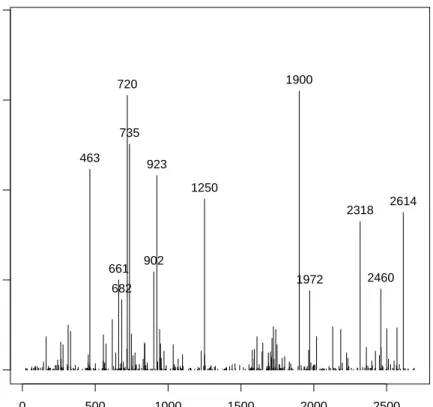
Results For each of the 500 bootstraps we computed the TSPs and stored the

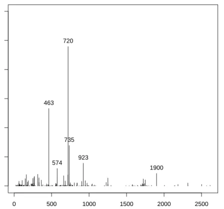
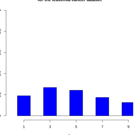
selected gene pairs. We are also intersted in the appearance of the single genes, because this can be useful to determine the importance of a single gene in the detection of the specic cancer tissues. It can be further used if we are interested in classication based on single genes or if we look for a set of genes correlatd to the disease. Figure 1 shows the frequency of appearance for each genes among all gene pairs. We keept only genes that had a signicant frequency of appearance relatively to the other pair (>8%).

0 500 1000 1500 2000 2500 0.0 0.1 0.2 0.3 0.4 0.5 0.6 Genes Frequency

Frequency of appearance of single genes in the tsp for the leukemia cancer dataset

463

574 923 720

735

1900

Figure 1: Frequency of appearance of the single gene in the pairs selected by the TSP over 500 bootstrap resamples from the dataset Leukemia cancer, only the

genes whose appearance where above 8% where hold.

The genes 463, 574, 712, 735, 923 and 1900 are the genes that appear the most

often in the pair of genes selected by the TSP over the bootstrap. If one would be interested on a subset of genes correlated with the disease, the TSP would provide such a set. This set could be improved by using other methods since the

(17)

TSP used in this way would only provide a clue about which genes should the set contains.

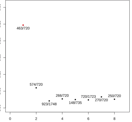
The most interesting part of the simulation is the frequency of appearance of the pairs selected by the TSP as we focus our study on the robustness of the method. We are interested in the freqeuncy of appearance of the original gene pair of the TSP in the bootstraped datasets. Figure 2 presents the resulted TSP over the bootstraped data as well as the number of times the gene appeared. We keept only pairs that had a signicant frequency of appearance relatively to the other pair (>5%). ● ● ● ● ● ● ● ● 0 2 4 6 8 0.00 0.05 0.10 0.15 0.20 0.25 0.30

Frequency of appearance of gene pairs in the tsp for the leukemia cancer dataset

Pair of genes Frequency 463/720 574/720 923/1748 266/720 148/735 720/1723 270/720 250/720 ●

Figure 2: Frequency of appearance of the pairs of gene selected by the TSP over

500bootstrap resamples from the dataset Leukemia cancer, we ploted only pairs

whose frequency was at least 5%. The pair with the red dot represents the pair

selected by the TSP on the original data set.

(18)

most often in the bootstrap of the Leukemia cancer dataset. We see that the pair

(463,720) which was detected by the TSP on the original dataset appears often

among the TSPs computed on the bootstrap, indeed this frequency is about25%of

the time and is much more bigger than the second best frequency of appearance. Which is attaigned by the pair (574,720) and is about 7%. The other pairs of

genes computed by the TSP on the bootstrap have a frequency about3%. Finally

we observe that the genes 720 appears in three quarter of the pairs, which makes

it very interesting for the study of this dataset because of its high correlation with the disease. On the other hand Figure 2 showed also that the gene 1900 was of

interest, but it doesn't appear in the pair of genes for the selected threshold of appearance.

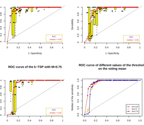
Figure 3 shows the ROC curve for the TSP applied on the leukemia cancer dataset.

These results showed good properties of the TSP. We want to make the reader sensible to the fact that they hardly depends on the dataset we used. We briey introduce another dataset and analyse the sensibility of the TSP to changes in the same way as for the leukemia cancer dataset.

This dataset is based again on tumor sample, but this time from breast cancer. It contains 78 observations, which consists of patients who developped a distance

metastase within 5 years (they were labeled as "diseased") and patients who

re-mained healthy for at least5years after their original diagnosis (they were labeled

as "healthy"). We have 34 "diseased" patients and 44 "healthy". The number of

genes was 24481. We did the ltering and the bootstrap in the same way as for

the leukemia cancer dataset.

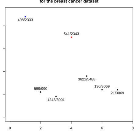
The TSP computed on the original dataset of breast cancer selected the pair of genes(541/2343). Actually the maximum score∆was achievied by two pairs. The

tie was separated by the second score Γin order to pick one pair. Figure 4 shows

the frequency of appearance of the pair of genes that appeared the most often. We see that the pair(498/2333), which was ranked second on the original dataset,

appears more often than the pair that was ranked rst. Inversely the top ranked pair from the original dataset is ranked second with the bootstrap resampling. The top pair on the boostrap sample appears slighty more than 8% of the time,

whereas the frequency of the top pair based on the original dataset appears is approximately of 7%.

There are other pairs of gene highlighted by the bootstrap which were not detected by the TSP. There were5pairs which appear around 2−3% of the time. In total

(19)

● ● ● ● ● ● ● ● ● ● ● ● ● ● ● ● ● ● ● ● ● ● ● ● ● ● ● ● ● ● ● ● ●● ● ●

ROC curve for the TSP on the leukemia cancer dataset

1−Specificity Sensibility AUC: median = 0.95 0 0.2 0.4 0.6 0.8 1 0 0.2 0.4 0.6 0.8 1 ● ● ● ● ●● ● ● ●● ● ● ●●● ● ● ● ● ● ● ● ● ● ● ● ● ● ● ● ● ● ● ● ● ● ● ● ● ● ● ● ● ● ●● ● ● ● ● ● ● ● ● ● ● ●●● ●

Figure 3: ROC curve for the TSP on the leukemia cancer dataset. The red line represents the median of the sensibility. The grey line stands for the line with interecept0 and slope 1.

If we add the frequencies of the7gene pairs selected (whose frequencies are above 0.02%) we obtain only25% of the total frequency, which is a very low percentage.

Indeed, this means that 3times over4a perturbation of the dataset leads to pairs

that doesn't belong to the selected pair of genes (with the threshold) over the boostrap.

We see on the second dataset that the TSP is much more sensible to perturbations than on the rst dataset. The pair provided by the TSP on the original dataset appears much more often among the bootstrap made on the rst set than among the bootstrap made on the second set. This sensitivity highly depends on the setup of the dataset. We saw that, on the second dataset, two pairs of genes reached the maximum score∆, which makes this two pairs very competitive to each other.

(20)

● ● ● ● ● ● ● 0 2 4 6 8 0.00 0.02 0.04 0.06 0.08

Frequency of the pair genes in the tsp for the breast cancer dataset

Pair of genes Frequency 498/2333 599/990 1243/3001 541/2343 3621/5488 130/3069 21/3069 ● ●

Figure 4: Frequency of appearance of the pairs of gene selected by the TSP over

500 bootstrap resamples from the dataset Breast cancer, we ploted only pairs

whose frequency was at least 2%. The pair with the red dot represents the pair

selected by the TSP on the original data set. The pair with the blue dot achieved the same score ∆as the top pair but was ranked second with respect to the score Γ.

This problem will be analysed with more precision in a later section.

The simulation provided in this section highlights the power of the bootstrap, it allowed us to obtain a large amount of datasets based on an original dataset and showed us how the TSP reacted to changes in the dataset. We note that the changes were totally arbitrary, every observation could have been removed or observed several times. We actually observed lack of robustness of the TSP for low perturbations as well as for important perturbations in the dataset.

(21)

mathemat-ical denition. But before we will present some basic notions of robustness in a general meaning. Then we will adapt them to the special case of the TSP in order to see why and how changes in the data can modify the pair selected by the TSP. Finally, we will derive a function to calculate the number of observations that can be added (and removed) from the dataset leaving the TSP unchanged. This func-tion will be a funcfunc-tion of the setting of the dataset (the number of observafunc-tions, the number of observations in each group, the size of the groups,etc).

2.3.2 Basic notion of robustness

The main goal of statistic is to analyse dierent kinds of datasets and to be able to draw useful estimations from them in order to learn from what we observed and to allow predictions with a certain amount of accuracy (often also estimated from the data). The main weakness of most estimators is their reaction to perturbations on the dataset, i.e., they stay in a neighborhood of the original estimation or if they hardly dier when adding an atypical observation to the dataset. A eld of statistics deals with such problems, it studies how an estimator reacts to changes in the dataset and provides new estimators which are supposed to be less sensitive to perturbations. This branch of statistics is relatively new to the other elds but it gained a lot of importance in the last 30 years. This eld is the so called

Robust statistics and seeks to provide methods that are competitive with popular statistic methods but which are less aected by outliers or small derivations from the model's assumptions.

In this section we present two basic notions of robust statistics. The rst notion is based on the sensitivity of an estimator to a single observation, which represents the inuence of adding a new observation to the dataset. It measures the variation of the estimator as a function of the single observation added to the dataset. The second notion we present computes the largest proportion of atypic points that the dataset can contain such that the estimator still yields accurate information about the parameter of interest.

Sensitivity curve and inuence function The rst notion we present is called the Sensitivity Curve, and as its name shows, it deals with sensitivity. An impor-tant point in robustness is to compute how a new observation added to the dataset can modify our estimations. The sensitivity curve is based on this point of inter-est. Let us denote by _θˆ_n₍_{x1, . . . , x}_n₎ _{the estimation of the paramter} _θ _{based on a}

sample of sizen composed of the observationsx1, . . . , xn. We writex0 as the new

(22)

The sensitivity curve (SC) for the sample of sizencomposed ofx1, . . . , xnis dened as follows SCn(x0) = ˆ θn+1(x1, . . . , xn, x0)−θˆn(x1, . . . , xn) 1/(n+ 1) = (n+ 1) ˆθn+1(x1, . . . , xn, x0)−θˆn(x1, . . . , xn . (5)

The sensitivity curve computes the dierence of the estimation of θ based on the

original dataset plus the new observation x0 and the estimator based exclusively

on the original dataset. This quantity is then scaled by the number of observation of the largest set (n+ 1). It represents the inuence of the observation x0 on the

estimator of θ.

The inuence function is calculated for a niten, we note that there exists an

ex-tension to this quantity asntends to innity. This is the so called Inuence Function,

which measures the inuence of an observation x0 as n tends to innity. In this

paper we will concentrate us only on the sensitivity curve, for more details about the inuence function see [5].

The next point that we will present computes the largest number of observations we can add to the dataset such that the pair provided by the TSP remains un-changed.

Breakdown point We have seen how to compute the inuence of a new obser-vation to the estimate. We will now introduce another quantity which allow us to compute the largest amount of atypical points (contamination) that the data may contain such that the estimate_θˆ_{will still give an accurate estimation of the}

param-eter θ. We are interested in the proportion of incorrect observations (arbitrarily

large observation) that can be contained in the dataset such that the estimator still gives accurate estimation of the parameter of interest. By accurate we mean that the estimator cannot take arbitrarily large values. As for the sensitivity curve there exist a distinction in the case of nite and unnite sample size. Here we are interested only in the nite version as we deal with dataset for which the sizen is

known and nite. For more details on the unnite case see [5].

The nite-sample breakdown point (FBP) of an estimate _θˆ _{for the sample} _S ₌ {x1, . . . , xn}is the largest proportion∗n(ˆθn, S)of data points that can be arbitrarily

replaced by outliers without _θˆ_n _{leaving a set which is bounded and also bounded}

(23)

We can express this more formally. For this we deneXm as the set of all datasets

S0 of size n having n−m elements in common with the set S. Mathematically

this is expressed by Xm ={S0 : |S0|=n, |S∩S0|=n−m}. Then ∗_n(ˆθn, S) = m∗ n , where

m∗ = max{m≥0 : ˆθ(S0) bounded and also bounded away from ∂Θ∀S0 ∈ Xm}.

We will now biey discuss this denition. First, the set Xm stands for all possible

perturbations of the original dataset withm observations being modied. Then it

searches the largest amount of data (largest m) such that the estimation remains

bounded and bounded away from the boundary in the worst case. The worst case is nding the lowest number of observations m we need to modify such that

the estimation doesn't provide anymore a good information for the parameter of interest, i.e., the lowest amount of data we need to modiy such that the estimator "breaks".

We give a quick example to enhance the intuition on this notion. Let us suppose we have a set of independant observations following a Normal distribution, i.e.,

(X1, . . . , Xn)

iid

∼ N(µ, σ2₎ _{and we are intested in estimating the mean} _µ _{of this}

sample. An usual way is to use the maximum likelihood estimator, which is dened as ˆ µn = 1 n n X i=1 Xi.

This estimator has a breakdown point of 0, indeed by changing any of thexi we

can make µˆn arbitrarily large. Robust statistics suggest to estimate the mean

through the median of the sample (X1, . . . , Xn). In this case, if we change only

one of thexi's it won't be enough to make this estimator arbitrarily large. In fact

the median has a breakdown point of0.5as we need to change at least the half of

the observations to make it arbitrarily large.

Moreover we note that for any estimator it is not possible to have a breakdown point higher than 0.5. This is due to the fact that, if more than a half of the

observations are contamined, then we can't distinguish between the data from the true model and the perturbated data.

In the next subsection we analyse the robustness of the quantities used for the derivation of the TSP, i.e., the score ∆and the rank score Γ.

(24)

2.3.3 Analytical study of the robustness for ∆ and Γ

The TSP's procedure in selecting the pair of genes is entirely based on the com-putation of the quantities ∆and Γ. In order to study the property of robustness

for the TSP it is necessary to rst investigate this property for the score and the rank score.

Let us suppose the dataset is dened as S = {(x1, y1), . . . ,(xn, yn)}, where xi

stands for the gene expression of the observation i and yi as an indicator for the

group to which the sample ibelongs, we write yi = 1 if it belongs to the groupC1

and yi = 2 if it comes from the group C2. Let us write∆ = ∆n(S) andΓ = Γn(S)

to emphasis that these quantities depends on the current datasetS. We begin with

the score∆. We compute the sensitive curve and discuss the breakdown point for

this parameter and then we will do the same for the rank score Γ.

Robustness of ∆ We analyse the robustness of ∆ for a given pair of genes.

Without loss of generality we write this pair as(i, j)and we suppose thatpij(C1)> pij(C2), which denes the classication rule expressed in (4). We dene the

fol-lowing quantities n1 = |C1|, n2 = |C2|, k1 = |{k ∈ C1 : xi,k > xj,k}| and k2 =

|{k ∈C2 :xi,k > xj,k}|. The probabilities pij(Ci) are estimated by pˆij(Ci) = _nki_i for

i= 1,2. The score becomes in this case ∆ij(S) = k1 n1 − k2 n2 .

A new observation is characterised by the vector (x0, y0) and by denition the

sensitive curve is dened as SCn(x0) = 1 n+ 1 k1+I (x0, y0)∈M1 n1+I(y0 = 1) −k2 +I (x0, y0)∈M2 n2+I(y0 = 2) − k1 n1 −k2 n2 ! , whereM1 ={(x, y)∈S:y = 1, xi < xj}and M2 ={(x, y)∈S :y= 2, xi < xj}.

We can suppose suppose thaty0 = 1 (the procedure is similar with y0 = 2). With

the assumption that pij(C1)> pij(C2), the sensitivity curve becomes 1 n+ 1 k1+I (x0, y0)∈M1 n1+ 1 − k2 n2 − k1 n1 + k2 n2 ! .

Moreover we suppose that the part in the absolute value is positive, so we can omit the absolute value (need to put a −1 if it is not the case), and nally the

(25)

sensitivity curve is given by SCn(x0) = 1 n+ 1 _n 1I (x0, y0)∈M1 −k1 n1(n1+ 1) .

We see that the sensitivity curve is, in this case, a line with a jump when(x0, y0)∈/ M1. On each side of the jump the curve takes two dierent values

−k1

n1(n1+ 1)(n+ 1)

and n1−k1 n1(n1+ 1)(n+ 1)

.

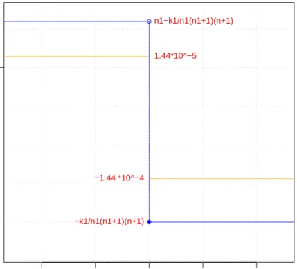
The graph of the sensitivity curve for the parameter ∆ is shown in Figure 5. We

observe that these values remain bounded (the absolute value never exceed 1), so

the inuence of one observation is bounded and cannot make the sensitivity curve explode.

For example on the breast cancer dataset with the assumption that y0 = 1 and pij(C1) > pij(C2), we obtain the two values 1.44·10−5 and −1.44·10−4 for the

inuence function. On the other hand, if we suppose that y0 = 2 but pij(C1) > pij(C2) still holds, we obtain the values 3.19·10−5 and −3.29·10−4. Here the

division byn1(n1+ 1)(or n2(n2+ 1)in the case where y0 = 2) reduces signicantly

the inuence of one observation.

The computation of the breakdown point for the case of the parameter ∆ is not

obvious. Indeed, the parameter ∆ranges in [0,1], so the boundary of this

param-eter is {0,1}. Given a dataset S ={(x1, y1), . . . ,(xn, yn)}dened as previously. If

all observations from the group C1 except one satises the rule R(i, n) > R(j, n)

and no observation from the group C2 satises it, then the score would be n1_n1−1.

If we construct a second dataset S0 equal to S but where the observation from

the group C1 which didn't satised the rule is replaced by an observation which

satises the rule, then the score ∆ will be 1. From the denition we presented

about the breakdown point of an estimator, the breakdown point of ∆ would be 0as the estimator reaches the boundary. But the estimators computed on the set S0 still give accurate results about the pair (it provide perfect classication on the

current dataset) and dier from the previous estimator only by 1

n1. For this reason

setting the breakdown point of ∆ to 0 is a severe decision. Another denition of

the breakdown point should be used here in order to allow more exibility when reaching the boundary.

During the computation of the sensitivity curve we came accross an important property of ∆ which has to be highlighted. As we introduced a new observation x0, we computed the dierence of the scores ∆ij(S)−∆ij(S0). This gives an

(26)

−4 −2 0 2 4

Sensitive curve for Delta

x0i−x0j SCn(x0) ●● ● −k1/n1(n1+1)(n+1) n1−k1/n1(n1+1)(n+1) −1.44 *10^−4 1.44*10^−5 0

Figure 5: The red line represents the sensitive curve for the parameter Delta in an arbitrary dataset. The orange line represents this curve applied on the leukemia cancer dataset, where we supposed thatpij(C1)> pij(C2) and y0 = 1

If we suppose that k1 n1 >

k2

n2 the dierence is given by ∆ij(S)−∆ij(S0) =    n1−k1 n1(n1+1), if xi,0 < xj,0 −k1 n1(n1+1), otherwise. (6) Here we supposed thatx0 ∈C1, the result is similar withx0 ∈C2. In our study we

worked with bootstrap to investigate the robustness of the method. In bootstrap, the notion of replacing is of interest since the size of the resample dataset is the same as the size of the original dataset. In this case where only one observation is

(27)

replaced, the dierence in the score is given by ∆ij(S)−∆ij(S0) =            −1 n1, if xi,0 < xj,0 1 n1, if k1−1 n1 > k2 n2 2k1 n1 − 2k2 n2 − 1 n1, if k1−1 n1 < k2 n2. (7) The dierence 2k1 n1 − 2k2

n2 is, because of the assumption made, quite small. Indeed

we supposed that k1−1 n1 < k2 n2 which is equivalent to 2k1 n1 − 2k2 n2 < 1 n1. Finally we

can conclude that ∆ij(S)−∆ij(S0) ≤ _n11 . The case when the inequality is strict

occurs when there is a change in the sign of k1−1

n1 − k2

n2, i.e. when pij(C1) becomes

less than pij(C2). This shows that the inuence of one observation of the group C1 (resp. C1) on the score is bounded by _n11 (resp. _n21 ). And thus the inuence of

one observation is bounded by max 1

n1,

1

n2

.

Robustness of Γ Let us analyse the rank score. As a new observation was

introduced to the dataset, the rank score will take into account a new element and will be modied. The sensitivity curve of this parameter is

SCn(x0) = _n₊₁1 P yn=Cm R(i,n)−R(j,n) + R(i,x0)−R(j,x0)I(y0=1) |Cm|+I(y0=1) − P yn=Cm R(i,n)−R(j,n) + R(i,x0)−R(j,x0)I(y0=2) |Cm|+I(y0=2) − P yn=Cm R(i,n)−R(j,n) |Cm| − P yn=Cm R(i,n)−R(j,n) |Cm| ! .

It is obvious that this function remains bounded. Indeed the values which allow to compute the rank score are the rank of the gene expressions within the proles. The ranks within each prole will stay bounded and can't be larger than the total number of genes, so the dierence between the rank of two genes within one prole will be less than the total number of genes (so it can't become arbitrarily lage). Furthemore the number of indices on which we sum is nite. Finally we use the fact that a nite sum of bounded number is also bounded. We can use 2(n+ 1)P as a

bound for the sensitivity curve ofΓ, whereP stands for the number of genes.

In this case again, the notion of breakdown point we presented won't yield any interesting results. Indeed, the values of Γ ranges in [0,∞[. It is possible for Γ

to reach 0 in the case where all the patient's genes expressions would have the

(28)

unintersting for the classication procedure as the indivual's gene expression have the same order in both groups. Moreover, the value ofΓ can't be made arbitrarily

large as it uses a nite sum of rank values (also nite).

2.3.4 Adaptation of the basic notion of robustness for the method TSP

We dened two important notions to analyse the robustness of parameters. In this paper we are mostly interested in the robustness of the TSP, i.e., we need a notion to dene robustness for a method instead of parameters. In the next section we will present an adaptation of the sensitivity curve and the breakdown point for the method TSP.

Sensitivity curve The denition for the sensitive curve that we presented is for the case of a continuous estimator. In our case we want to analyse the inuence of an observation on the TSP. The TSP yields a pair of genes, which is a discrete element inN×N. Adding an observation to the dataset may have dierent impacts,

it can reduce or increase the accuracy rate of the TSP (if the gene pair matches or not with the classication rule determined by the TSP), or much worse, it can produce changes in the results of the TSP by using a dierent pair for the classication rule. In this report we are interested in the second case (altough it is highly related to the loss of accuracy, as we will see later).

We thus adapt the notion of sensitivity curve to that case. As we are intested only in changes in the resulting gene pair, it is natural to consider two events, either the pair provided by TSPx0 is the same as for the TSP or the pair is a dierent one.

We mean by TSPx0 the TSP based on the augmented dataset, i.e., the original

dataset including the observation x0. The sensitive curve will be dened in the

following way. We set it to 1 if TSPx0 yields the same result as the original TSP

and to 0 otherwise. We denote the adaptation of the sensitive curve to the TSP

by SCTSP and we dene it as

SCTSP =I pair(TSPx0) =pair(TSP)

,

where the function pair(·) returns the pair of the TSP and I(·) represents the

indicator function.

This adaptation will be very useful to study the sensitivity of the TSP to a new observation, as it will compute if the TSP will remain unchanged (SCTSP = 1)

or if another pair of gene will be selected by the method (SCTSP = 0). We will

(29)

dataset (number of observations, number of observations in each group, etc). This relationship will be analysed and precisely determined as a function of the setting in a later section.

We note that SCTSP may be easily adapted to the case where we add a set of

observation to the dataset instead of a single observation.

Breakdown point Here we are interested in the breakdown point for the TSP, and as before we have to adapt this notion to this special case. We dene the breakdown point for the TSP, denoted by BPTSP, as the largest proportion of data

that can be replaced by contaminated observations (will be dened more precisely in the next section) such that the pairs of genes provided by the TSP computed on the perturbated dataset are the same as the TSP computed on the original dataset. Mathematically this can be written as

BPTSP = _n1 max arg max

n0_∈{₀_,₁_,...,n_} min S_n0⊂{1,...,n} I pair(TSPS_n0) = pair(TSP) ,

where TSPSn0 stands for the TSP computed on the dataset where the elementsxi,

with i∈Sn0, have been replaced by arbitrary observations.

Some words to the denition. We took the indicator function on the pairs of both TSP, the one computed on the original dataset and the one computed on the con-tamined dataset in order to see when the pairs of genes provided by both TSP will be dierent.

Second we took the minimum over all possible subsets of indices from{0,1, . . . , n}

because we want to see if the gene pair will change in any of the case where the number of contamination is n0. If for one subset from {0,1, . . . , n} the TSP

com-puted on the contamined dataset diers from the original gene pairs, the indicator function will be equal to 0. Thus we want that the number of perturbations

al-lowed such that the gene pair doesn't change to be lower than the current value of

n0. The value ofn0 won't be considered, because forn0 the indicator function is0.

We note that for n0 = 0 the indicators function is 1 and thus argmax will contain 0 and not n0, so 0 ≤ BP_TSP < n0 (for n00 > n0 the minimum of the indicators

function will be 0 because we can choose the same subset of index as in the case

where the indicator function was 0 for n0 and add a pertubation which let the

indicator function to be equal to 0).

Afterwards we take the max over all possible amounts of contamination such that the genes pairs don't change (they are given by the arg max function) in order to

have the largest number of contamined data that can be introduced to the dataset such that the gene pair stays the same as for the original dataset.

Finally, we divide this number by the total number of observations n to obtain a

(30)

2.3.5 Analytical study of the robustness of the TSP

In this part we are intersted in computing analytically the robustness of the TSP. Firstly we will study the inuence of a new observation on the pair of genes selected by the TSP on the original dataset and show that this inuence depends highly on the setup of the dataset and express it explicitly as a function of the setup. Secondly we will give the value of the breakdown point of the TSP using a sample where this value can be computed easily and we will show that it is equal to0.

Inuence of a new observation We suppose we performed the TSP on a dataset and that the gene pair resulting is given by(i, j). Without loss of generality

we suppose that pij(C1) > pij(C2), so for a new observation xn+1, we assign it to

the group C1 if xi,n+1 < xj,n+1 and to the groupC2 otherwise.

We set the following notation, n1 = |C1|, n2 =|C2|, k1 = |{k ∈ C1 : xi,k > xj,k}|

and k2 =|{k ∈C2 :xi,k > xj,k}|.

The score of the pair(i, j) is dened by∆ij =

_n1k1 − k2_n2

.

Suppose the second best TSP is represented by (k, l)(here we suppose that there

are no ties, i.e., ∆kl < ∆ij). We want to see the inuence on a new observation

on the gene pair yield by the TSP. More precisely we are interested to see when the pair (i, j) will become ranked second instead of rst. Suppose we add a new

observation x0 to the dataset and without loss of generality we can suppose that x0 comes from the group C1. We distinguish two cases

1. xi,0 > xj,0 :

The new observation matches with the decision rules of the current TSP. Then the TSP will remain unchanged and its score will increase and be equal to ∆0_ij = k1+ 1 n1+ 1 − k2 n2 >∆ij,∆0kl.

The TSP will select again the pair(i, j).

2. xi,0 < xj,0 :

This case is more interesting since the classication rule of the TSP doesn't match with the relative ordering expression of the new observation. Thus the computation of the score will be aected. Indeed the score for the pair(i, j)

will become lower as we add an individual to the group C1 whose relative

(31)

of the pair (i, j) would be given by ∆0_ij = k1 n1+ 1 − k2 n2 <∆ij.

Now the point is to see if this new individual will make the score of the second pair bigger. We suppose it is the case (otherwise we would use the pair that has the higher score and whose classication rule matches with the relative ordering of the new observation for this pair), i.e., xk,0 > xl,0. Since

the new observation matches with the classication rule of the TSP based on the pair (k, l)the score ∆kl will increase and be

∆0_kl = k₁0 + 1 n1+ 1 − k 0 2 n2 ,

wherek0₁ andk0₂ are dened as for the rst pair but with indices(k, l)instead

of (i, j). The results of the TSP on the original dataset will change if the

score of the second pair (the one for wich the classication rule matches with the relative ordering of the new individual) becomes higher than the score of ∆ij, i.e., if k₁0 + 1 n1+ 1 − k 0 2 n2 > k1 n1+ 1 − k2 n2 , which is equivalent to k0₁+ 1 n1 + 1 − k 0 2 n2 − k1 n1+ 1 − k2 n2 >0.

This is a necessary and sucient condition such that the pair (i, j) is not

selected anymore by the TSP. Let us dene the fonction

f(k1, k2, k01, k 0 2, n1, n2) = k0₁+ 1 n1+ 1 − k₂0 n2 − k1 n1+ 1 − k2 n2 . (8)

This function depends highly on the setup of the dataset as it depends explicitely on the variables (k1, k2, k01, k20, n1, n2), which are quantities specic to the analysed

dataset.

Here we supposed that the new observation belonged to the group C1. If the

(32)

worked in the same way, butn2 would have been increased to n2+ 1instead of n1.

Supposing this observation would be unfavorable to the classication rule of the pair (i, j) (the pair (i, j)would misslcassie this observation) but not for the pair (k, l), then k0₂ would be increased to k₂0 + 1. We note that adding an observation

in the group C1 or in the groupC2 has not the same inuence on the score when

|C1| 6=|C2|.

We also have to be careful on the fact that for the derivation of f we supposed

thatpij(C1)> pij(C2). If this inequality is inversed, the interpretation of favorable

observation to a pair of genes will have a dierent meaning, in the sense that the relative order of the gene expressions will be inversed.

We saw that if the new observation's relative ordering gene expressions matches with the classication rule of the best pair, the TSP selects the same pair. But in the case where the relative ordering gene expressions of this new individual doesn't match with the classication rule, then changes in the selected pair of genes may occur. The pair that could become ranked rst is one for which the relative ordering gene expression of this new observation matches with the classication rule of this pair, otherwise the score of this pair won't be increased and can't become higher than the best score. In order to have this pair ranked rst, its score must become higher than the updated best score (taking into account that a new observation is added to the dataset). The function f(·) gives information if the selected gene

pair will be subject to changes with the simple condition f(·) > 0 (this means a

dierent gene pair will be selected).

We can make an extension to this function to nd how many observations we can add to the current dataset such that the selected gene pair will remain unchanged. We consider the worst case, i.e., add observations whose relative ordering genes ex-pressions don't match with the classication rule but match with the classication rule of the second best pair (which will become the top ranked one in this case). We have to split the derivation of this function in two cases as for the derivation of the function f. First we suppose that the new observations come from the group C1 and dene F1 is dened as

F1(k1, k2, k10, k 0 2, n1, n2, x) = k₁0 +x n1+x − k 0 2 n2 − k1 n1+x − k2 n2 .

Then we seek for the largest positive integer x such that the function F1(k1, k2, k01, k

0

(33)

In the same way, for new observations which come from the group C2 we dene

the function F2 with the same parameters as for F1 as F2(k1, k2, k10, k 0 2, n1, n2, x) = k₁0 n1 − k 0 2+x n2+x − k1 n1 − k2 n2+x .

Here we supposed that pij(C1) > pij(C2). The case where pij(C1) < pij(C2) will

be similar but we need to change the indices, i.e., k1, k2, n1 and n2 will become k2, k1, n2 and n1 respectively.

These functions seek how many observations from group C1 or C2 wich are

un-favorable to the best pair but un-favorable to the second one, one can add such that the orignal pair remains ranked rst, i.e., the largest integer x such that F1(k1, k2, k01, k

0

2, n1, n2, y)<0,∀ y≤x and equivalently forF2.

One can combine these two functions in order to obtain the largest amount of data one can add such that the pair of genes remains unchanged in the worst case, i.e., if the new observations came from the group C1 or C2. We note that if the

sizes of the two groups are equal, then it has no inuence if the observations come fromC1 or C2. If the groups' sizes are not equal then the worst case will be when

unfavorable indviduals come from the group with the lowest size as its inuence will be of size 1

Ci, i = 1,2. We can combine the functions F1 and F2 to have

a general form for the largest number of observations one can add such that the gene pair stays the same. We dene the functionF, which stands for this quantity,

as

F(k1, k2, k10, k 0

2, n1, n2, x) = max{x: F1(y), F2(y)<0, ∀y ≤x}. (9)

We saw a function that is able to compute if a new observation may produce changes in the gene pair selected and we also saw an extension to compute how many observations, which are unfavorable to the top pair but favorable to the second pair (seen as the worst case), can be added to the dataset without producing changes to the selected gene pair. We will apply these two functions on the dataset of leukemia cancer and breast cancer and compare their values with the result we found when we used the boostrap resampling. We will rst apply them on the breast cancer dataset as it will give a direct calculation to compute the breakdown point fo the TSP and will highlight the eect of ties on the choice of the best pair.

When applying the TSP on this dataset a tie will occur. Indeed the two pair of genes (498,2333) and (541,2343) will be selected with the same score ∆ = 0.82,

(34)

this case, if we add only one observation which is favorable to one of the pair but unfavorable for the second pair, it is obvious that the rst pair will be selected and be the only one to achieve the best score. Here we don't consider the second pair

(498,2333) and see when the score of the third best pair will become ranked rst.

The third best pair of this dataset is(3621,5488)with a score∆ = 0.79. For these

two pairs of genes we have the setting k1 = 40, k2 = 3, k10 = 40, k 0

2 = 4. In this

case the group C2 contains less observations than the groupC1, so an unfavorable

observation for the top TSP will have a higher inuence if this observation belongs to the group C2. Here we are interested in the worst case, so we suppose that

the observation comes from the group C2, the size of the rst group n1 as well

as the number of people in the group satisfying the rule of the rst TSP k1 and

of second TSP k₁0 won't change, in addition the number of people in the second

group satisfying the rule of the rst tspk2 won't change too. However the number

of people in the second group that satises the rule of the second TSP will be incremented by 1 (as the size of the second group). After some computation we

obtain that F = 0. Which means that the second considered TSP will become as

good as the rst one and a tie will occur. It may happen that this TSP will have an average ranking dierence higher that for the rst TSP and nally be picked as the best pair by the TSP. We note that this analyse could have been done in the same way when we remove one observation from the dataset. This example illustrates well how adding a single observation might change the pair of genes selected by the TSP. This highlights the sensibility of the TSP and gives an accurate function of its sensibility depending on the setting of the analyzed dataset.

Through the computation of the function F on the dataset of breast cancer we

observed that adding an observation that doesn't match with the top TSP but which matches with the second best TSP might produce changes on the gene pair that the TSP selects. This means that, in the worst case, the largest proportion of data we can perturbate such that the TSP produces the same result is0%, for this

reason the breakdown point of the TSP in, a general case, is 0. It is clear that it

highly depends on the dataset we used, and for this reason we gave an adaptation of the breakdown point to a specic dataset. Moreover the maximum score∆was

reached by two pairs, it was intuitively obvious that adding an observation that matches only with one of the classication rule would have produced changes on the score ∆ and thus modify the selected pair of genes.

We will apply these functions on the dataset leukemia cancer. The best score is

∆ = 0.98and is reached by the pair(463,720), the second highest score is∆ = 0.96

for the pair(1900,2234). The values of the parameters for the function of interest

are n1 = 47, n2 = 25, k1 = 46, k2 = 0, k01 = 0 and k 0

2 = 24. By the same way as