Improving the representation of hydrological connectivity in conceptual models

Mitteilungen

Heft 110

INSTITUT FÜRHYDROLOGIE UNDWASSERWIRTSCHAFT

V. T. NGUYEN

Hydrological Connectivity in Conceptual

Models

Von der Fakult¨at f¨ur Bauingenieurwesen und

Geod¨asie der Gottfried Wilhelm Leibniz Universit¨at Hannover

zur Erlangung des akademischen Grades Doktor-Ingenieur

Dr.Ing.

-genehmigte Dissertation

von

Van Tam Nguyen, M.Sc. geboren am 11.08.1985 in Bac Ninh

Referent: PD. Dr.-Ing. J¨org Dietrich

Korreferent: Prof. Dr. rer. nat. habil. Martin Volk Tag der Promotion: 03.03.2020

First of all, I would like to thank Prof. Dr.-Ing. Uwe Haberlandt and PD. Dr.-Ing. J¨org Dietrich for giving me a chance to do this PhD at the Institute of Hydrology and Water Resources Management. I would like to thank my PhD supervisor, PD. Dr.-Ing. J¨org Dietrich, for his scientific guidance and support during my PhD. His guidance and knowledge have helped me to have a scientifically sound approach to new problems and to become a SWAT developer. I am also very thankful for his support in my personal life during my research.

Special thanks go to Dr.-Ing. Ana Callau for offering me the HIWI position during my Master’s study at WAWI. The working experience that I had during this time has helped me in learning FORTRAN, R, statistics, which were very useful for my PhD research.

I want to thank all of my colleagues at the Institute of Hydrology and Water Re-sources Management for the fruitful discussion during the ”Klausurtagungen”. To Bhu-mika Uniyal, I would like to thank for her help in proof-reading all of my manuscripts and also for her contribution to my research. Special thanks go to all of the anonymous reviewers of my papers, whose comments significantly improved the quality of the papers. I would also like to thank Stefan and Prajna for sharing the office with me. I want to thank Ana, Mathias, Anne, Prajna, Bruno, Bora, Luisa, Bhumika, Quynh, Stefan, and Hannes for sharing their fun time with me during the last four years.

Last but not least, I would like to thank my parents for their sacrifice for my education, to my wife and my son for supporting me spiritually throughout the PhD research.

I, Van Tam Nguyen, hereby declare that:

1. I know the regulations for doctoral candidates and have met all the requirements. I agree with an examination under the provisions of the doctoral regulations. 2. I have completed the thesis independently; used materials by others shall be listed

in the references

3. I did not pay any monetary benefits for regards to content.

4. This work contains no material which has been accepted for the award of any other degree or diploma at any other university or tertiary institution.

5. The same or partly similar work has not been submitted at any other university or academic institution.

6. I agree that my thesis can be used for verifying the compliance with scientific stan-dards, in particular using electronic data processing programs.

The relevant permission that might be needed from the journals to reproduce the published works are granted from the copyright holders.

Leipzig, March 5, 2020

Understanding hydrological connectivity is one of the main objectives in hydrological research. Hydrological models have been proved to be an efficient tool for a better under-standing of hydrological connectivity. Conceptual models have shown certain advantages compared to physically-based distributed models in terms of data requirement and compu-tational time. However, the hydrological connectivity in conceptual models is usually not well represented. In this study, the Soil and Water Assessment Tool (SWAT) was selected for further improvements to have a better representation and simulation of hydrological connectivity.

SWAT is a semi-distributed hydrological model used to simulate the effect of land use management practices on water, sediment, and nutrient yields at a basin scale. SWAT has been tested and applied worldwide. However, the non-spatial characteristic of the hydrologic response unit (HRU) concept used in SWAT has been identified as one of the main disadvantages for modeling hydrological connectivity. In this study, the hydrologic routing subroutine of SWAT was examined and the groundwater subroutine was modified to account for hydrological connectivity in porous and karst-dominated aquifers.

Results show that the current hydrologic routing subroutines of SWAT are not able to simulate hydrological connectivity between river segments in the river network. The Muskingum routing method in SWAT could (1) cause unphysical oscillations in the simu-lated streamflow and (2) overestimate the evapotranspiration loss in the river and results in a hydrologic disconnectivity during low flow periods. For improving the representation of hydrological connectivity in the subsurface porous aquifer, the multicell aquifer model was proposed and incorporated into SWAT. The modified model, the so-called SWAT-MCA model, was validated in two basins located in Niedersachsen, Germany. The results show that the SWAT-MCA model could well simulate the regional groundwater flow and return flow from aquifer to stream. For improving the representation of hydrological con-nectivity in the karst-dominated aquifer due to interbasin groundwater flow (IGF) was added to SWAT, the SWAT IGF was developed. The developed model was applied in

could well represent the hydrological connection due to interbasin groundwater flow in karst areas. The modified models, SWAT-MCA and SWAT IGF could be applied for other regions to regional groundwater flow in porous aquifer and IGF in karst-dominated aquifers.

Das Verst¨andnis der hydrologischen Konnektivit¨at ist eine der Hauptaufgaben in der hydrologischen Forschung. Hydrologische Modelle haben sich als effizientes Werkzeug f¨ur ein besseres Verst¨andnis der hydrologischen Konnektivit¨at erwiesen. Konzeptmodelle haben im Vergleich zu physisch basierten verteilten Modellen hinsichtlich Datenbedarf und Rechenzeit gewisse Vorteile gezeigt. Die hydrologische Konnektivit¨at in in konzeptuellen Modellen ist jedoch nicht gut dargestellt. In dieser Studie wurde das Soil and Water Assessemnt Tool (SWAT) f¨ur weitere Verbesserungen ausgew¨ahlt, um die hydrologische Konnektivit¨at besser darstellen und simulieren zu k¨onnen.

SWAT ist ein semi-verteiltes hydrologisches Modell, das verwendet wird, um die Auswirkungen von Landmanagementpraktiken auf den Wasser-, Sediment- und N¨ahrstoffhaushalt in Flussgebieten zu simulieren. SWAT wurde weltweit getestet und angewendet. Die nichtr¨aumlichen Eigenschaften des in SWAT verwendeten HRU-Konzepts (Hydrologic Response Unit) wurden jedoch als einer der Hauptnachteile f¨ur die Modellierung der hydrologischen Konnektivit¨at identifiziert. In dieser Studie wurde das Unterprogramm f¨ur hydrologisches Routing von SWAT weiter getestet und das Grundwasser-Unterprogramm wurde modifiziert, um die hydrologische Konnektivit¨at in por¨osen und karstdominierten Aquiferen zu ber¨ucksichtigen.

Die Ergebnisse zeigen, dass die aktuellen Unterprogramme f¨ur hydrologisches Rout-ing von SWAT keine hydrologischen Verbindungen im Flussnetz simulieren k¨onnen. Das Muskingum-Routing-Verfahren in SWAT k¨onnte (1) unphysikalische Oszillationen im simulierten Stromfluss verursachen und (2) den Evapotranspirationsverlust im Fluss ¨

ubersch¨atzen und zu einer hydrologischen Diskontektivit¨at bei niedrigen Abfl¨ussen. Zur Verbesserung der Darstellung der hydrologischen Konnektivit¨at im unterirdischen por¨osen Aquifer wurde das Multicell-Aquifer Modell in SWAT integriert. Das modifizierte Mod-ell, das sogenannte SWAT-MCA ModMod-ell, wurde in zwei Flussgebieten in Niedersachsen validiert. Die Ergebnisse zeigen, dass das SWAT-MCA Modell den regionalen Grund-wasserfluss gut simulieren kann. Um die Darstellung der hydrologischen Konnektivit¨at im

gebiet im S¨udwesten des Harzes in Deutschland angewendet. Das Modell wurde mit dem beobachteten Abfluss des Flusses und der Karstquelle validiert. Die Ergebnisse zeigen, dass der SWAT IGF die hydrologische Verbindung aufgrund des Grundwasser-flusses zwischen den Becken in Karstgebieten gut darstellen k¨onnte. Die modifizierten Modelle SWAT-MCA und SWAT-IGF k¨onnten f¨ur andere Regionen eingesetzt werden, um IGF in por¨osen und karstdominierten Aquiferen zu simulieren.

Schl¨usselw¨orter: SWAT, hydrologische Konnektivit¨at, Hochwasserf¨uhrung, Karst, Grundwasserfluss

a.m.s.l above mean sea level

BGR Bundesanstalt f¨ur Geowissenschaften und Rohstoffe DEM Digitial Elevation Model

DWD Deutscher Wetterdienst ETa Actual Evapotranspiration HRU Hydrologic Response Unit IGF Interbasin Groundwater Flow

LU Landscape Unit

MCA Multicell Aquifer Model

NLWKN Nieders¨achsische Landesbetrieb f¨ur Wasserwirtschaft, K¨usten- & Naturschutz NSE Nash–Sutcliffe Efficiency

PBIAS Percentage BIAS

1 Introduction 1

1.1 Research Problem and Motivation . . . 1

1.2 Literature Review . . . 4

1.2.1 SWAT . . . 4

1.2.2 Current approaches and challenges for simulating hydrological con-nectivity with SWAT . . . 8

1.3 Research Objectives and Methodology . . . 14

1.4 Thesis Structure and Author Contribution . . . 15

2 Verification and Correction of the Hydrologic Routing in the SWAT 22 2.1 Introduction . . . 23

2.2 Theoretical Background . . . 24

2.2.1 Variable Storage Method . . . 24

2.2.2 Muskingum Method . . . 25

2.3 Hydrologic Routing with SWAT . . . 26

2.3.1 Variable Storage Routing Subroutine . . . 26

2.3.2 Muskingum Routing Subroutine . . . 27

2.4 Verification Examples. . . 28

2.4.1 Study Area and Data . . . 28

2.4.2 Simulation Scenarios . . . 28

2.4.3 Results and Discussions . . . 30

2.7 Acknowledgments . . . 34

2.8 Conflicts of Interest . . . 34

3 Modification of the SWAT Model to Simulate Regional Groundwater Flow Using A Multi-Cell Aquifer 37 3.1 Introduction . . . 38

3.2 Methodology . . . 41

3.2.1 The original groundwater module of SWAT. . . 41

3.2.2 The modified groundwater module . . . 42

3.2.3 Input data preparation . . . 46

3.2.4 Model integration framework . . . 46

3.3 Case Study . . . 47

3.3.1 Study areas and data . . . 47

3.3.2 Spatial discretization . . . 50

3.3.3 Calibration and validation strategy . . . 52

3.4 Results and Discussion . . . 54

3.4.1 Calibrated parameter values . . . 54

3.4.2 Overall water balance . . . 54

3.4.3 Stream discharge . . . 55

3.4.4 Groundwater levels . . . 57

3.5 Conclusion and Recommendations . . . 63

4 Modeling Interbasin Groundwater Flow in Karst Areas: Model Devel-opment, Application, and Calibration Strategy 71 4.1 Introduction . . . 72

4.2 Methodology . . . 75

4.2.1 The original SWAT model . . . 75

4.3.1 Study area and data . . . 80

4.3.2 Geology . . . 83

4.3.3 Hydrogeology . . . 83

4.4 Model setup, calibration and validation . . . 86

4.4.1 Model setup . . . 86

4.4.2 Calibration and validation strategy . . . 86

4.5 Results and discussion . . . 89

4.5.1 Sensitivity analysis and best calibrated parameter set . . . 89

4.5.2 The role of using MOD16 ETa and multi-site streamflow data and for model calibration . . . 90

4.5.3 Simulated streamflow . . . 93

4.5.4 Simulated karst groundwater storage variation . . . 96

4.6 Conclusions and recommendations. . . 97

5 Conclusion and Future Outlooks 107 5.1 Conclusions . . . 107

5.1.1 Hydrological connectivity in the river network . . . 108

5.1.2 Subsurface hydrological connectivity in porous aquifer . . . 108

5.1.3 Subsurface hydrological connectivity in karst-dominated aquifer . . 109

5.2 Future Outlooks. . . 110

5.2.1 General . . . 110

5.2.2 Original SWAT model . . . 110

5.2.3 SWAT-MCA model . . . 111

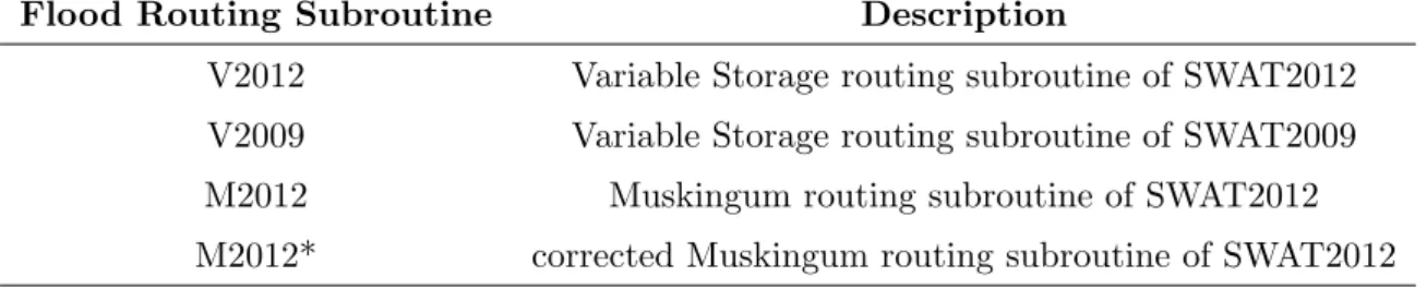
2.1 List of the hydrologic routing subroutines used for this study.. . . 30

2.2 Model performance statistics for flood event 1 (17 January 1990 to 17 April 1990, Figures 2.2a,b) and flood event 2 (18 December 1990 to 1 February 1991, Figures 2.2c,d). . . 32

3.1 The overlapping area matrix between HRUs and cells . . . 46

3.2 Characteristics of the study areas . . . 48

3.3 Best calibrated parameter values of the original SWAT and SWAT-MCA models . . . 53

3.4 Performance of the calibrated SWAT and SWAT-MCA model (in terms of streamflow at the Oetzm¨uhle and S¨uttorf gauging stations) . . . 60

4.1 Selected parameter for sensitivity analysis and sensitivity ranking . . . 87

4.2 List of calibration scenarios and the corresponding weights in the objective function . . . 88

4.3 Selected parameters for calibration and the best parameter values . . . 89

4.4 Model performance statistics and characteristics of the 95PPU band. Num-bers outside parentheses indicate values of the calibration period while numbers inside parentheses indicate values of the validation period. . . 92

1.1 The water cycle and global distribution of water resources (Oki and Kanae, 2006). . . 2

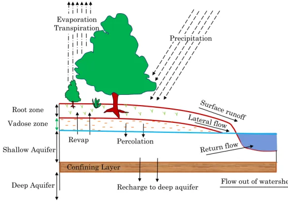
1.2 Land phase processes in SWAT (modified from Neitsch et al., 2011) . . . . 5

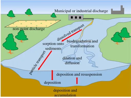
1.3 Stream processes in SWAT (modified from Neitsch et al., 2011) . . . 6

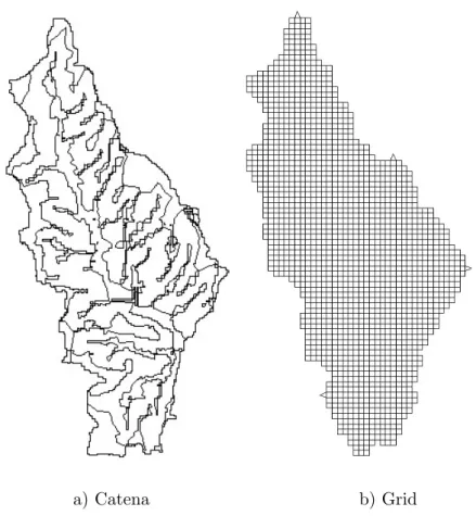
1.4 Discretization of the basin using a) the catena and b)grid approaches in SWAT (Arnold et al., 2010). . . 10

1.5 Hydrological connectivity between different landscape units in the grid-based SWAT model (Arnold et al., 2010). . . 10

1.6 The schematic description of the SWAT-MODFLOW model (Kim et al., 2008). . . 11

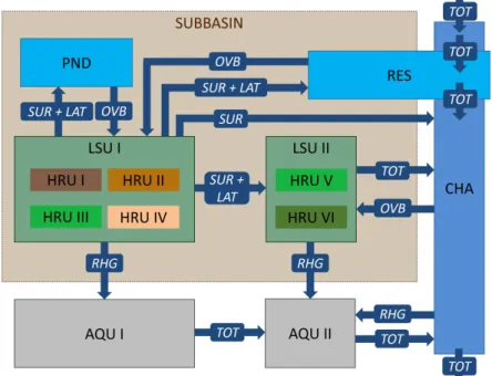
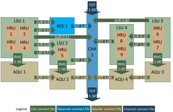
1.7 Hydrological connectivity between different spatial objects in SWAT+ (Bieger et al, 2017). SUR is surface runoff, LAT is lateral flow, RHG is groundwater recharge, TOT is total flow. . . 12

1.8 Represention of hydrological connectivity between upland area, floodplain, and river in SWAT+ (Bieger et al, 2019). . . 13

2.1 Location of the Weser River segment and its tributary rivers. . . 29

2.2 Simulated outflow at the Vlotho gauging station for two flood events using (a,c) V2009 and V2012 and (b,d) M2012 and M2012*. . . 31

2.3 Flow duration curves of the simulated streamflow (logarithmic scale) at the (a) Welsede, (b) Afferde, and (c) Uchtdorf gauging stations during 1990–2000 with M2012 and M2012*. . . 33

the surface run-off, lateral flow, return flow from local aquifer, return flow from regional aquifer, and regional groundwater flow, respectively. The numbers indicate the average annual water balance components in mil-limeters per year in the Wipperau (numbers outside parentheses) and the Neetze (numbers inside parentheses) basins . . . 43

3.2 Schematic representation of the multicell aquifer model . . . 45

3.3 Integration framework of the soil and water assessment tool–multicell aquifer model . . . 47

3.4 Location and digital elevation model (DEM) of the Neetze and Wipperau basins . . . 49

3.5 Delineation of the subbasin and the regional groundwater aquifer of (a) the Neetze basin and (b) the Wipperau basin . . . 51

3.6 Observed and simulated streamflows from (a, c) the original SWAT models and (b, d) the SWAT-MCA model at the Oetzm¨uhle (Wipperau basin) and S¨uttorf (Neetze basin) gauging stations during 1980–2007. A portion of the semi-log plot was shown in normal plot (a) to show that it is difficult to see the quality of the simulated low flow with normal plot. SWAT = soil and water assessment tool; MCA = multicell aquifer . . . 56

3.7 Flow duration curves of the observed and simulated streamflows at the Oetzm¨uhle gauging station from the SWAT and SWAT-MCA models dur-ing 1980–2007. SWAT = soil and water assessment tool; MCA = multicell aquifer . . . 57

3.8 Time series plots of the observed and simulated groundwater levels during 1980–2007 and statistical indices (Nash–Sutcliffe efficiency [NSE], percent bias [PBIAS], and ratio of the root mean square error to the standard deviation of measured data [RSR]): (a) good match between observed and simulated groundwater levels, (b) mismatch between the time of occurrences of the high and low groundwater levels between observed and simulated groundwater levels, and (c) well reproduced of short- and long-term ground-water fluctuations. Boxplots of the absolute differences between simulated and observed groundwater levels are attached to the right of the time series plots . . . 58

the extractions wells located nearby . . . 62

4.1 Conceptual models of the SWAT IGF model. (A) the conceptual model for the non-karst area (the original conceptual model of SWAT), (B) the con-ceptual model for the karst area (modified from SWAT).Qsurf is the surface runoff,Qlatis the lateral flow,wrevapis the groundwater revap,wrshallow and

wrdeep are the shallow and deep groundwater recharge, respectively, other variables were described in text. . . 77

4.2 The study area with the Digital Elevation Model. . . 81

4.3 Distribution of (A) land use/land cover, (B) soil, and (C) slope with sub-basin numbers in the study area. . . 82

4.4 Geological map of the study area (BGR). Location of the faults and dif-ferent types of streams were identified according to Th¨urnau (1913) and Grimmelmann (1992). More information about the geological cross-section could be found in Grimmelmann (1992). . . 84

4.5 Time series plot of MOD16 ETa and simulated ETa from the calibration scenario S2. . . 91

4.6 Scatter plots of NSEET a versus NSEQLindau, NSEQScharzf eld and

NSEQKupf erhutte¨ for behavioral simulations in the calibration scenario

S2 (from 2000-2005). The red cross indicates the simulation corresponding to the best parameter set. . . 91

4.7 Times series plots of streamflows and flow duration curves (attached to the right of the respective time series plot) of the observed and the sim-ulated streamflow from SWAT IGF during the calibration period (2000-2005). The simulated streamflow at the Rhume spring (blue line) using the original SWAT was added in (G). For a better visualization, only the 95PPU band for the Rhume spring was shown. . . 94

4.8 Times series plots of streamflows and the flow duration curves (attached to the right of the respective time series plot) of the observed and the simulated streamflow from SWAT IGF during the validation period (2006-2010). The simulated streamflow at the Rhume spring (blue line) using the original SWAT was added in (G). . . 95

Introduction

1.1

Research Problem and Motivation

Water covers most of the earth’s surface and it is one of the vital sources of life. The water cycle (Figure 1.1) is one of the governing processes on Earth and it plays an important role in the Earth’s climate self-regulation (Allen, 2009; Nordstrom et al., 2005). Water is abundant on Earth, however, only 2.5% of the total water amount is freshwater. In addition, only a small portion of freshwater is accessible (Oki and Kanae, 2006). Fresh-water distribution on Earth varies with space and time (Piao et al., 2010). The uneven distribution of water could cause water shortage or flood (Imamura and Van To, 1997;

Oki and Kanae, 2006; Shiklomanov, 1991). Water shortage or flood has been identified as one of the controlling factors of social and economic welfare (Gleick, 1993; Lehner et al., 2006).

The natural redistribution of water on the Earth’s surface and subsurface occurs in the form of surface and subsurface flows. Different landscape units could be hydrologically connected by surface and/or subsurface flows (Garven,1995;Tockner et al.,1999). The hy-drological connection between different landscape units is called hyhy-drological connectivity. Hydrological connectivity describes the linkage between upstream with downstream, sur-face with subsursur-face, hillslope with riparian zone, terrestrial with aquatic (Covino,2017). These linkages can occur at various spatio-temporal scales (local to regional scales) and different directions (vertical, lateral, longitudinal) (Covino,2017). These linkages control the transport of water and solute and affect the hydrological cycles.

In a broader sense, hydrological connectivity refers to the transfer of water and its associated components (e.g., nutrients and sediments) between different landscape units

Figure 1.1: The water cycle and global distribution of water resources (Oki and Kanae,

2006).

(e.g., hillslope, floodplain, and river) or between different components of the hydrolog-ical cycle (Pringle, 2003). It should be noted that there exist different definitions of hydrological connectivity depending on the geomorphic domain (Bracken et al., 2013). Understanding the hydrological connectivity between different landscape units could help water resource managers in formulating appropriate management strategies, especially in terms of transboundary water resources management (Bracken et al., 2013). For ex-ample, identifying the critical source areas which contribute most of the pollutants and their hydrological connection with other landscape units are crucial for developing effec-tive measures. This has been long of interest in the hydrological community (e.g.,Covino,

2017;Niraula et al.,2013;Srinivasan and McDowell,2009). In the region where interbasin groundwater flow is significant, understanding the transport of water and solute fluxes via interbasin groundwater flow (subsurface connectivity) has significant implications for water management.

There have been various studies focused on improving the understanding the hydro-logical connectivity. Different approaches could be used to understand different types of hydrological connectivity, ranging from experimental studies to numerical study using hydrological models (Bracken et al., 2013). This study focuses on developing modeling

tools to have a better representation and understanding of hydrological connectivity. In this study, the term “hydrological connectivity” is restricted to (1) the lateral surface and subsurface flow between different landscape units and (2) the vertical flow between the soil layers and the aquifer.

Various models have been developed to help in understanding and predicting the hy-drological connectivity, ranging from lumped conceptual to distributed physically-based models. Lumped conceptual models consider a whole basin as a single unit. They only consider the vertical hydrological connectivity between different vertical storages (e.g., percolation of water between different soil layers, and groundwater recharge). Some ex-amples of these models are the NAM (Nielsen and Hansen, 1973), PDM (Moore, 2007) and VHM (Willems, 2014) models.

In conceptual (semi-)distributed models, a basin is divided into subbasins and fur-ther divided into smaller spatial units. One of the most frequently used methods for basin delineation is the hydrologic response unit (HRU) concept (Leavesley et al., 1983). Within the HRU concept, each HRU has a unique combination of land use, soil type and slope within a subbasin. HRU is considered to be homogeneous in hydrologic response. A single HRU can be scattered over different areas in a subbasin. Some models of this type are the Soil and Water Assessment Tool (SWAT, Arnold et al.,1998), Hydrologiska Byr˚ans Vattenbalansavdelning (HBV, Bergstr¨om, 1992), Precipitation-Runoff Modeling System (PRMS, Markstrom et al., 2015), and Hydrological Predictions for the Environ-ment model (HYPE, Lindstr¨om et al., 2010). In these models, hydrological connectivity is considered (1) between different soil layers and aquifers within an HRU (vertical hy-drological connectivity), and (2) between subbasins via the stream network (longitudinal hydrological connectivity). In general, the subsurface of each HRU in conceptual mod-els is assumed as a system of connected reservoirs. These reservoirs represent the water storage in different soil zones and in the aquifers. Flow between these reservoirs is often simulated using simple routing equations. There is no lateral hydrological connectivity (surface and subsurface flows) between HRUs. Flow from each HRU is assumed to be independent of other HRUs and it does not interact with each other. The summation of all HRUs’ responses within a subbasin is considered as the subbasin’s response.

Other delineation approaches were also used in (semi-)distributed models. For exam-ple, the Water Erosion Prediction Project (WEPP, Flanagan and Nearing, 2015) model divides a basin into hillslope, channel, and impoundment. The mesoscale hydrologic model (mHM,Kumar et al., 2013;Samaniego et al.,2010) divides a basin into grid cells. However, both of the aforementioned models do not model the subsurface flow between

different landscape units.

With physically-based distributed models, e.g., the Modular Three-Dimensional Finite-Difference Ground-Water Flow Model (MODFLOW, Harbaugh and McDonald,

1996), HydroGeoSphere (Therrien et al., 2009), and OpenGeoSys (Kolditz et al., 2012), the study area is divided into grid cells and surface and subsurface flow between grid cells is simulated by using physical equations (e.g, Darcy’s law and Richards’ equation). However, the disadvantages of physically-based distributed models are the extensive re-quirement of data and computational capacity.

Compared to physically-based distributed models, conceptual (semi-)distributed mod-els often require less simulation time while preserving the spatial heterogeneity in land use and soil type. The main disadvantage of the conceptual distributed models is the lack of lateral hydrological connectivity between HRUs or subbasins (e.g., SWAT, HBV, HYPE). Some studies have compared the performance between physically distributed models and conceptual distributed models (e.g., Devia et al., 2015; Liu et al., 2016). Results show that more complex models do not always guarantee a better result than simpler models. SWAT is a conceptual distributed model for assessing the impact of land use man-agement practices on water, sediment, and chemical yields at a basin-scale (Arnold et al.,1998). SWAT has been widely used and tested worldwide (Arnold and Fohrer,2005). SWAT has been proved to be a unique model which could incorporate various natural and anthropogenic processes (e.g., dynamic land use change, sediment, and nutrients flow in karst) (Arnold and Fohrer,2005;Pai and Saraswat,2011;Nerantzaki et al.,2015). There-fore, improving SWAT for simulation of hydrological connectivity will bring a significant benefit to the SWAT community.

1.2

Literature Review

1.2.1

SWAT

In SWAT, a basin is divided into subbasins which are further divided into HRUs according to different land use, soil type, and slope classes (Arnold et al.,1998;Neitsch et al.,2011). One HRU could be scattered across different places within a subbasin. SWAT simulates two phases of the hydrological cycle, the land phase (HRU-related processes, Figure 1.2) and the routing phase (stream-related process, Figure 1.3). The HRU-related processes are evapotranspiration, surface runoff, lateral flow, infiltration, percolation, groundwater

recharge, return flow, etc. (Figure 1.2). The stream processes are flow and transport in the stream network (Figure1.3).

Evaporation Transpiration

Precipitation

Revap _Percolation

Recharge to deep aquifer Flow out of watershed

Shallow Aquifer Deep Aquifer Confining Layer Vadose zone Root zone 1

Figure 1.2: Land phase processes in SWAT (modified from Neitsch et al.,2011)

The land phase considers hydrological connectivity in the vertical direction between different soil layers and between the soil zone and the aquifers. The soil layers and aquifers are represented as a system of connected reservoirs. Infiltrated rainfall first fills up the uppermost soil layer. If the water content in the soil layer exceeds its field capacity, the excess water will be routed to the next soil layer. The infiltrated water that exits the bottom of the soil profile is considered as groundwater recharge. Groundwater recharge is split into shallow groundwater and deep groundwater recharge. Recharge to the deep aquifer is considered as a loss from the system (Figure1.2).

Municipal or industrial discharge sorption onto sediments biodegradation and transformation dilution and diffusion

deposition and resuspension deposition

deposition and accumulation non-point discharge

Figure 1.3: Stream processes in SWAT (modified fromNeitsch et al., 2011)

The daily water balance for the soil zone (all soil layers) for an HRU (Figure 1.2) is calculated as follows (Arnold et al.,1998; Neitsch et al.,2011):

SWi =SWi−1+Pi−Qsurf −ETa−wseep−Qlat (1.1)

where SWi and SWi−1 (mm H2O) are the total soil water content in the soil on day i

andi−1, respectively, Pi (mm H2O) is the amount of precipitation on dayi,Qsurf,ETa,

w_seep, and Q_lat (mm H2O) are the amount of surface runoff, actual evapotranspiration,

percolated water out of the soil profile, and the total amount of lateral flow from all soil layers on dayi.

In each HRU, infiltrated water is routed from the topsoil layer to the aquifer using the routing technique described below. Water percolates from the upper soil layer to the lower soil layer if the water content in the upper soil layer exceeds the field capacity. In this case, the amount of drainable water volume SWly,excess (mm H2O) from the upper

soil layer is calculated as follows:

SWly,excess =SWly−F Cly (1.2)

whereSWly and F Cly (mm H2O) are the soil water content and the field capacity of the

lower soil layer,wper,ly (mm H2O), is:

wper,ly =SWly,excess·(1−e−∆t/T Tper) (1.3)

where ∆t (hour) is the number of hours in a day, and T Tper (hour) is the travel time for

percolation within the respective soil layer, which is expressed as follows:

T T_per = SATly−F Cly Ksat

(1.4) whereSATly (mm H2O) is the amount of water in the soil when the soil is fully saturated,

K_sat (mm/h) is the saturated hydraulic conductivity of the soil layer.

Percolated water out of the lowest soil layer and infiltration losses from secondary channels, ponds and wetlands are considered as groundwater recharge, wseep (mm H2O).

The hydraulic connection between the lowest layer, the unsaturated zone, and the shallow aquifer is represented by the groundwater delay time, δgw (days). Therefore, the actual

amount of groundwater recharge, w_rchrg,i (mm H2O), to both shallow and deep aquifers

during dayi is:

wrchrg,i = (1−e−1/δgw)·wseep+e−1/δgw ·wrchrg,i−1 (1.5)

wherewrchrg,i−1 is the total groundwater recharge on previous day. The total groundwater

recharge is separated into shallow, wrchrg,sh, and deep groundwater recharge, wrchrg,deep,

as follows:

w_rchrg,sh = (1−β_deep)·w_rchrg,i (1.6)

w_rchrg,deep =β_deep·w_rchrg,i (1.7)

where βdeep is the portion of recharge to the deep aquifer. The daily water balance for

the shallow aquifer is expressed as follows:

aqsh,i =aqsh,i−1+wrchrg,sh−Qgw−wrevap−wpump (1.8)

where aqsh,i and aqsh,i−1 (mm H2O) are the amount of water in the shallow aquifer on

revaporation, and pumping, respectively. Recharge to the deep aquifer is considered as loss from the system.

In SWAT, there is no lateral hydrological connectivity between HRUs due to their non-spatial characteristics. Summation of all HRU responses within a subbasin is considered as a subbasin response. Streamflow generated from upstream subbasin is routed to down-stream subbasin using a simple hydrological routing method. Streamflow is considered as the only hydrological connection between subbasins in SWAT.

1.2.2

Current approaches and challenges for simulating

hydro-logical connectivity with SWAT

Some studies have been conducted to improve the representation of hydrological con-nectivity in SWAT. These studies focus on improving (1) the hydrological concon-nectivity between river segments in the river network (e.g., Kim and Lee, 2010; Nguyen et al.,

2018a; Pati et al., 2018), (2) the hydrological connectivity between HRUs within a sub-basin (e.g., Arnold et al., 2010; Rathjens et al., 2015), and (3) hydrological connectivity in the subsurface (e.g., Bailey et al.,2016; Kim et al., 2008).

Kim and Lee(2010) found that the Muskingum routing method used in SWAT is inap-propriate for estimating the shape and magnitude of the flood wave as it moves from the upstream to downstream. The Muskingum method used in SWAT (Cunge,1969; USDA,

2004) could cause unphysical oscillations during the recession and an underestimation of the peak flows. The modified Muskingum method proposed by Kim and Lee (2010) was proved to be an error-free and a robust approach for stream routing. Nguyen et al.(2018a) integrated SWAT with the HEC-RAS model (which uses the hydraulic method for flood routing). HEC-RAS model has been widely used to simulate hydrological connectivity in the stream network. Results showed that the coupled model could represent changes of the flood waves better than the original SWAT.Pati et al.(2018) replaced the Muskingum routing method in SWAT with the variable parameter MacCarthy-Muskingum (VPMM). They found that the VPMM could account for the nonlinear behavior of the flood wave in small slope and steep slope channels.

For improving the representation of hydrological connectivity between landscape units in SWAT, different landscape delineation techniques were proposed, e.g., the catena and grid delineation techniques (Arnold et al., 2010;Rathjens et al., 2015). With these delin-eation techniques, the spatial location of each landscape unit is identified for flow routing. Therefore, the flow routing between these landscape units is possible. With the catena

approach, the basin is divided into a divide, hillslope, and valley bottom (Figure 1.4). Hydrological connectivity between the divide, hillslope, and valley bottom can be rep-resented by surface runoff, lateral flow, and groundwater flow between these landscape units (Figure ?? Arnold et al., 2010). The catena approach could be used to assess the impact of upslope management on downslope landscape units (Arnold et al., 2010).

In the catena approach, flow is routed according to the surface topographic gradient (from the divide to the hillslope and the valley bottom). In lowland regions, however, the topographic gradient could be small and groundwater flow might not follow the surface topographic gradient. In addition, the catena approach only simulates hydrological con-nectivity within a basin. Therefore, the catena approach is not applicable for modeling interbasin groundwater flow. Furthermore, there is no general technique for an automatic delineation using the catena approach (Arnold et al.,2010; Gallant and Dowling, 2003).

In the grid base version, the basin is divided into grid cells. Surface and subsurface runoff follow surface topographic gradient. Hydrological connectivity between grid cells was simulated in the same way as the catena approach (Figure 1.5). The application of the grid version of SWAT, however, is not difficult for large river basins (Arnold et al.,

2010). This is because of the extensive requirements of input data and computational capacity (Arnold et al.,2010).

Lumped HRU Catena Grid

Figure 3. Landscape delineation methods used on the USDA‐ARS Brushy Creek watershed (17.3 km

).

Divide Hillslope Floodplain Landuse SRO Channel SRO SROT

Rain

Rain + SRO

Soil

Ground water

B

T= Groundwater total SRO = Surface runoff total

S

T = Lateral soil flow total

BT S_T Soil P C C P P Hillslope Floodplain Land use SRO SROT

Rain + SRO

+ Flood

Figure 4. Processes considered in landscape routing units.

Shallow groundwater in this region has been evident since

the early farming days of the late 1800s, as shown by the

abundance of shallow hand‐dug wells across the Blackland

prairie. This shallow groundwater system has been studied

and shown to follow local topography at an average depth of

3 m. Recharge occurs through aerial infiltration at the outcrop

(Allen et al., 2005).

L

D

M

Lumped method.

For the lumped method, one HRU was

chosen to represent the watershed that consisted of the

dominant soil (Houston Black), dominant land use (pasture),

and average land slope.

HRU or hydrotope method.

To develop an HRU, the land

use and soils maps were overlaid and unique land use and soil

combinations were lumped together to form the HRU. The

average watershed slope was used for each HRU. In this

watershed, 155 HRUs with distinct soil and land

combinations were used (fig. 3). When an HRU is formed,

there is no reference to landscape location, and there is no

routing of flow across HRUs. Flow from each HRU is

summed to estimate water yield at the watershed outlet.

Catena method.

Existing methods to delineate landscape

units range from simple soil considerations to complex

methods using multivariate statistics and iterative

segmentation algorithms to interpolate the continuous

character of the landscape (Fluegel and Staudenrausch, 1999;

Blaschke and Strobl, 2003; Gallant and Dowling, 2003;

MacMillan et al., 2004; Moeller et al., 2008). Gallant and

Dowling (2003) point out that “there are no published

methods for mapping valley bottoms by automated

algorithms, although a number of methods exist that are

designed to map floodplains.” We searched for an effective

but simplified solution for large‐scale application and for

potential integration into SWAT. After an intensive

evaluation, we selected the slope position method (USDA,

1999) as a useful method to delineate landscape units (Volk

et al., 2007).

For this application, the watershed was divided into three

landscape units: the divide, hillslope, and valley bottom. A

a) Catena b) Grid

1

Figure 1.4: Discretization of the basin using a) the catena and b)grid approaches in SWAT (Arnold et al., 2010).

1436 TRANSACTIONSOFTHE ASABE

Lumped HRU Catena Grid

Figure 3. Landscape delineation methods used on the USDA‐ARS Brushy Creek watershed (17.3 km2_).

Divide Hillslope Floodplain Landuse SRO Channel SRO SROT

Rain Rain + SRO

Soil

Ground water

B_T= Groundwater total SRO = Surface runoff total S_T= Lateral soil flow total

BT ST Soil P C C P P Hillslope Floodplain Land use SRO SROT Rain + SRO + Flood BT ST Soil P C C P P SRO

Figure 4. Processes considered in landscape routing units.

Shallow groundwater in this region has been evident since the early farming days of the late 1800s, as shown by the abundance of shallow hand‐dug wells across the Blackland prairie. This shallow groundwater system has been studied and shown to follow local topography at an average depth of 3 m. Recharge occurs through aerial infiltration at the outcrop (Allen et al., 2005).

LANDSCAPE DELINEATION METHODS

Lumped method. For the lumped method, one HRU was chosen to represent the watershed that consisted of the dominant soil (Houston Black), dominant land use (pasture), and average land slope.

HRU or hydrotope method. To develop an HRU, the land use and soils maps were overlaid and unique land use and soil combinations were lumped together to form the HRU. The average watershed slope was used for each HRU. In this watershed, 155 HRUs with distinct soil and land combinations were used (fig. 3). When an HRU is formed, there is no reference to landscape location, and there is no

routing of flow across HRUs. Flow from each HRU is summed to estimate water yield at the watershed outlet.

Catena method. Existing methods to delineate landscape units range from simple soil considerations to complex methods using multivariate statistics and iterative segmentation algorithms to interpolate the continuous character of the landscape (Fluegel and Staudenrausch, 1999; Blaschke and Strobl, 2003; Gallant and Dowling, 2003; MacMillan et al., 2004; Moeller et al., 2008). Gallant and Dowling (2003) point out that “there are no published methods for mapping valley bottoms by automated algorithms, although a number of methods exist that are designed to map floodplains.” We searched for an effective but simplified solution for large‐scale application and for potential integration into SWAT. After an intensive evaluation, we selected the slope position method (USDA, 1999) as a useful method to delineate landscape units (Volk et al., 2007).

For this application, the watershed was divided into three landscape units: the divide, hillslope, and valley bottom. A

1

Figure 1.5: Hydrological connectivity between different landscape units in the grid-based SWAT model (Arnold et al.,2010).

Recent studies have integrated SWAT with the Modular Three-Dimensional Finite-Difference Ground-Water Flow Model (MODFLOW, Harbaugh and McDonald,1996) to improve the subsurface hydrological connectivity (Kim et al., 2008). In this integrated SWAT-MODFLOW model, SWAT is used to simulate land surface processes and soil-water dynamics. The percolated soil-water out of the soil profile from SWAT is considered as input (groundwater recharge) for the MODFLOW model Fig. 1.6. Results show that the couple SWAT-MODFLOW model was able to capture surface, subsurface flow, and river-aquifer interaction better than the original SWAT model (Kim et al.,2008). However, the MODFLOW model is a physically-based distributed groundwater model, which requires extensive input data and computational time. In regions where hydrogeological data are scared, the applicability and performance of the SWAT-MODFLOW are questionable.

Figure 1.6: The schematic description of the SWAT-MODFLOW model (Kim et al.,2008).

For improving the simulation of hydrological connectivity in karst areas, different ver-sions of the modified SWAT model were introduced, e.g., the KarstSWAT (Palanisamy and Workman, 2014) and KSWAT (Malag´o et al., 2016; Nerantzaki et al., 2015) models. The KarstSWAT model was developed mainly to represent the hydrological connection between sinkholes and springs (flow from sinkholes to springs). However, springs could be fed by diffuse recharge sources (areal recharge). The KSWAT model combines the two sub-models, the adapted SWAT model (Fig. 3, Malag´o et al., 2016) and the karst-flow model (Nikolaidis et al.,2013). The KSWAT model assumes that percolated water out of the soil profile is karst groundwater recharge (Fig. 3,Malag´o et al., 2016). This assump-tion might be invalid if the underlying aquifer of a subbasin is not entirely a karst aquifer

(e.g., Palanisamy and Workman, 2014). In this case, part of the infiltrated water could be hydrologically connected with streamflow in form of lateral flow and baseflow. In ad-dition, the adapted SWAT model does not differentiate different components of recharge (concentrated recharge and diffuse recharge). The karst-flow model uses the two-linear-storage reservoir model to represent the hydrological connection between recharge (which is simulated by theadapted SWAT model or from the original SWAT model) and spring. Discharge from the two reservoirs of the karst-flow model represents discharge from the conduit system and matrix (Malag´o et al.,2016). The KSWAT model does not differenti-ate between diffuse recharge and concentrdifferenti-ated recharge, and between matrix storage and conduit storage.

Figure 1.7: Hydrological connectivity between different spatial objects in SWAT+ (Bieger et al, 2017). SUR is surface runoff, LAT is lateral flow, RHG is groundwater recharge, TOT is total flow.

A recent revised version of SWAT, so-called SWAT+, has been developed and could be used to simulate hydrological connectivity in a very flexible way (Bieger et al, 2017). Within SWAT+, landscape units (LUs), HRUs, aquifer (AQU), channel (CHA), reservoir (RES), pond (PND) are considered as different spatial objects. The hydrological con-nection between these spatial objects is defined by the users (Figure 1.7). The aquifer delineation in SWAT+ is no longer tied to HRU and basin delineation. Due to the flexi-bility of SWAT+, it could be used to represent various kinds of hydrological connections. For example, SWAT+ was used to represent the hydrological connection between upland areas, flood plain, and river (Bieger et al, 2019). The SWAT+ model could potentially

be used to simulate interbasin groundwater flow by hydrologically connecting different aquifer units. However, the main difficulties with SWAT+ are the identification (or verifi-cation) of the hydrological connection and its magnitude between different spatial objects. For a large river basin that has numerous spatial objects, defining these connections could require extensive work.

Figure 1.8: Represention of hydrological connectivity between upland area, floodplain, and river in SWAT+ (Bieger et al, 2019).

Compared to the original SWAT model, the SWAT+ model has a higher number of model parameters due to the additional parameters for defining the hydrological connec-tion between different spatial objects. The uncertainty and equifinality of the addiconnec-tional parameters introduced in SWAT+ have not been fully explored. The magnitude of hy-drological connection between different spatial objects in SWAT+ is often difficult to validate directly/indirectly with measured/observed data. Therefore, the improvement of the SWAT+ model compared to the SWAT is in question.

Besides the major changes to the SWAT model structure as aforementioned, there have been several minor changes to improve the representation of hydrological connectivity. For example, (Rahman et al., 2016) modified the wetland module of SWAT to improve the representation of hydrological connectivity between riparian depressional wetlands, rivers, and aquifers. Hoang et al (2017) added a routing function to hydrological connect the upland areas with the riparian zones.

1.3

Research Objectives and Methodology

The main objective of this research is to improve the representation of hydrological con-nectivity in a conceptual distributed model, the Soil and Water Assessment Tool (SWAT) model. Specifically, the hydrological connectivity in this research refers to (1) the hydro-logical connection between river segments in the river network, (2) the regional groundwa-ter flow (ingroundwa-terbasin groundwagroundwa-ter flow) in porous aquifers, and (3) the regional groundwagroundwa-ter flow in karst-dominated aquifers.

To have a better understanding of the hydrological connectivity between river seg-ments in the river network, a detailed review and testing of the flood routing methods (Muskingum and variable storage method) of SWAT were conducted. The advantages and disadvantages of each routing method were discussed. The flood routing subroutines of SWAT were tested and validated separately from other subroutines. Testing the flood routing is one of the prerequisite objectives. This is because the flood routing is one of the main components of the model. It describes the changes of the flood waves along the river network. In other words, it describes the hydrological connection and the transformation of the flood wave as it moves from upstream to downstream sections of a reach.

To represent hydrological connectivity in porous aquifers, a different delineation tech-nique for the subsurface was proposed. The new delineation techtech-nique is expected to be simple and can be done automatically. In addition to the new discretization technique, a physically-sound approach for modeling hydrological connectivity between the subsurface units were proposed. For these aforementioned objectives, the Thiessen polygon technique was used for delineating the aquifer and Darcy’s law was used to simulate flow between aquifer units. A linear-storage reservoir was used to simulate the hydrological connection (via baseflow) between the aquifer and stream. The proposed model should be able to capture groundwater flow dynamics and surface runoff

For a better representation of hydrological connectivity in karst-dominated aquifers, a new discretization technique was introduced. The proposed discretization is expected to be independent of the surface topographic basin and be able to differentiate between karst and non-karst areas, karst recharge and discharge areas. To achieve these objectives, the discretization technique was based on the geological map and information obtained tracer tests. This is because the information obtained from tracer tests indicates the hydrolog-ical between different areas in the karst region. For modeling hydrologhydrolog-ical connectivity between different areas in karst areas, a two-reservoir model was proposed to represent different types of recharge and discharge in the karst area.

The overall results of this research are expected (1) to have a better simulation of hydrological connectivity between different river segments in the river network, and (2) to offer a compromise solution between physically based and conceptual models for simulat-ing regional groundwater in porous aquifers and (3) to have new approach for simulatsimulat-ing interbasin groundwater flow in karst-dominated aquifers. Although the SWAT model was specially selected in this study, the methodology presented here could also be applied for other conceptual distributed models.

1.4

Thesis Structure and Author Contribution

The remainder of this study was structured as follows.

1. Chapter 2 presents an approach for improving the simulation of hydrological con-nectivity between river segments in the river network with SWAT. In this chapter, the two flood routing techniques used in SWAT as well as their implementations in the code were reviewed and discussed. Application and testing of the revised code for flood routing in a reach segment located in the Wesser catchment were presented. Chapter 2 is the paper Verification and Correction of the Hydrologic Routing in the Soil and Water Assessment Tool published in Water (Nguyen et al., 2018). In this paper, the author contributed to the formulation of the idea, reviewing and developing the model code, and writing of the paper.

2. Chapter 3 presents a solution for improving the simulation of regional groundwater flow in porous aquifers. In this chapter, different approaches as well as their advan-tages and disadvanadvan-tages for simulating hydrological connectivity (regional ground-water flow) in porous aquifers were discussed. It is followed by a description of the modified groundwater module using the Multicell Aquifer Model (MCA). The case study section presents the application of the proposed models in two different sub-basins located in Niedersachsen, Germany. The remainders of chapter 3 represent the model results, discussion, conclusion and recommendations.

Chapter 3 is the paper Modification of the SWAT Model to Simulate Regional Groundwater Flow Using A Multi-Cell Aquifer published in Hydrological Processes (Nguyen and Dietrich, 2018). In this paper, the author developed the idea, wrote the paper, and set up test cases with the co-author. The model code was written by the author.

3. Chapter 4 introduces a new approach for improving the simulation of subsurface connectivity in karst-dominated aquifers. In this chapter, a detailed review of the karst system and its hydrological characteristics were presented. Different mod-els for simulating hydrological connectivities in the karst aquifer, especially inter-basin groundwater flow between different inter-basins, were discussed. It is followed by the formulation of the modified SWAT model using a two-reservoir model and the case study in southwest Harz Mountains, Niedersachsen, Germany. The result and discussions, conclusion and recommendations were presented in the remainders of chapter 3.

This chapter is the paper Modeling Interbasin Groundwater Flow in Karst Areas: Model Development, Application, and Calibration Strategy published in the Envi-ronmental Modelling and Software (Nguyen et al.,2020). In this paper, the author formulated the problem, test case study and wrote the paper with the co-authors. The model code was written by the author.

4. Chapter 5 summarizes the main findings from this research. In addition, this chapter also provides some suggestions for further improvements of the original SWAT as well as the modified SWAT model in this study.

Bibliography

Allen, P.A., 2009. Earth surface processes. John Wiley & Sons.

Arnold, J.G., Allen, P.M., Volk, M., Williams, J.R., Bosch, D.D., 2010. Assessment of dif-ferent representations of spatial variability on SWAT model performance. Transactions of the ASABE, 53(5), 1433-1443.

Arnold, J.G., Fohrer, N., 2005. SWAT2000: Current capabilities and research opportuni-ties in applied watershed modelling. Hydrological Processes, 19(3), 563-572.

Arnold, J.G., Srinivasan, R., Muttiah, R.S., Williams, J.R., 1998. Large area hydrologic modeling and assessment. Part I: model development. Journal of the American Water Resources Association, 34(1), 73-89.

Bailey, R.T., Wible, T.C., Arabi, M., Records, R.M., Ditty, J., 2016. Assessing regional-scale spatio-temporal patterns of groundwater–surface water interactions using a cou-pled SWAT-MODFLOW model. Hydrological Processes, 30(23), 4420-4433.

Bergstr¨om, S., 1992. The HBV model: Its structure and applications. Report Hydrology No. 4, Swedish Meteorological and Hydrological Institute.

Bieger, K., Arnold, J. G., Rathjens, H., White, M. J., Bosch, D. D., Allen, P. M., 2019. Representing the Connectivity of Upland Areas to Floodplains and Streams in SWAT+. JAWRA Journal of the American Water Resources Association.

Bieger, K., Arnold, J. G., Rathjens, H., White, M. J., Bosch, D. D., Allen, P. M., Volk, M., Srinivasan, R., 2017. Introduction to SWAT+, a completely restructured version of the soil and water assessment tool. JAWRA Journal of the American Water Resources Association, 53(1), 115-130.

Bracken, L.J., Wainwright, J., Ali, G.A., Tetzlaff, D., Smith, M.W., Reaney, S.M., Roy, A.G., 2013. Concepts of hydrological connectivity: research approaches, pathways and future agendas. Earth-Science Reviews, 119, 17-34.

Covino, T., 2017. Hydrologic connectivity as a framework for understanding biogeochem-ical flux through watersheds and along fluvial networks. Geomorphology, 277, 133-144. Cunge, J.A., 1969. On the subject of a flood propagation computation method

(Musk-ingum method). Journal of Hydraulic Research, 7, 205-230.

Devia, G.K., Ganasri, B.P., Dwarakish, G.S., 2015. A review on hydrological models. Aquatic Procedia, 4, 1001-1007.

Flanagan, D.C., Nearing, M. A., 1995. USDA-Water Erosion Prediction Project: Hillslope profile and watershed model documentation (Vol. 10, pp. 1603-1612). NSERL report. Gallant, J.C., Dowling, T.I., 2003. A multiresolution index of valley bottom flatness for

mapping depositional areas. Water Resources Res. 39(12), 1347.

Garven, G., 1995. Continental-scale groundwater flow and geologic processes. Annual Review of Earth and Planetary Sciences, 23(1), 89-117.

Gleick, P. H., 1993. Water in crisis. Pacific Institute for Studies in Dev., Environment & Security. Stockholm Env. Institute, Oxford Univ. Press.

Harbaugh, A. W., McDonald, M.G., 1996. User’s documentation for MODFLOW-96, an update to the US Geological Survey modular finite-difference ground-water flow model. US Geol. Surv., Open-File Rep. 96-485, 56.

Hoang, L., van Griensven, A., Mynett, A., 2017. Enhancing the SWAT model for simulat-ing denitrification in riparian zones at the river basin scale. Environmental modellsimulat-ing & software, 93, 163-179.

Imamura, F., Van To, D., 1997. Flood and typhoon disasters in Viet Nam in the half century since 1950. Natural Hazards, 15 (1), 71-87.

Kim, N. W., Chung, I. M., Won, Y. S., Arnold, J. G., 2008. Development and application of the integrated SWAT–MODFLOW model. Journal of Hydrology, 356(1-2), 1-16. Kim, N. W., Lee, J., 2010. Enhancement of the channel routing module in SWAT.

Hy-drological Processes, 24(1), 96-107.

Kolditz, O., Bauer, S., Bilke, L., B¨ottcher, N., Delfs, J. O., Fischer, T.,..., Park, C. H., 2012. OpenGeoSys: an open-source initiative for numerical simulation of thermo-hydro-mechanical/chemical (THM/C) processes in porous media. Environmental Earth Sciences, 67(2), 589-599.

Kumar, R., L. Samaniego, S. Attinger. 2013: Implications of distributed hydrologic model parameterization on water fluxes at multiple scales and locations, Water Resour. Res., 49(1), 360-379.

Leavesley, G.H., Lichty, R.W., Troutman, B., Saindon, L.G., 1983. Precipitation-runoff modelling system. User’s manual. USGS Water Resour. Inst., Report 83-4238.

Lehner, B., D¨oll, P., Alcamo, J., Henrichs, T., Kaspar, F., 2006. Estimating the impact of global change on flood and drought risks in Europe: a continental, integrated analysis. Climatic Change, 75(3), 273-299.

Lindstr¨om, G., Pers, C., Rosberg, J., Str¨omqvist, J., Arheimer, B., 2010. Development and testing of the HYPE (Hydrological Predictions for the Environment) water quality model for different spatial scales. Hydrology research, 41 (3-4), 295-319.

Liu, J., Liu, T., Bao, A., De Maeyer, P., Feng, X., Miller, S. N., Chen, X., 2016. As-sessment of different modelling studies on the spatial hydrological processes in an arid alpine catchment. Water resources management, 30(5), 1757-1770.

Malag´o, A., Efstathiou, D., Bouraoui, F., Nikolaidis, N.P., Franchini, M., Bidoglio, G., Kritsotakis, M., 2016. Regional scale hydrologic modeling of a karst-dominant geomor-phology: the case study of the Island of Crete. Journal of Hydrology, 540, 64-81.

Markstrom, S.L., Regan, R.S., Hay, L.E., Viger, R.J., Webb, R.M.T., Payn, R.A., and LaFontaine, J.H., 2015. PRMS-IV, the precipitation-runoff modeling system, version 4, U.S. Geological Survey Techniques and Methods.

Moore, R.J., 2007. The PDM rainfall-runoff model, Hydrology and Earth System Sciences, 11, 483-499.

Neitsch, S.L., Arnold, J.G., Kiniry, J.R., Williams, J.R., 2011. Soil and Water Assessment Tool theoretical documentation version 2009. Grassland, Soil and Water Research Lab-oratory, Agricultural Research Service and Blackland Research Center, Texas Agricul-tural Experiment Station, Temple, Texas.

Nerantzaki, S.D., Giannakis, G.V., Efstathiou, D., Nikolaidis, N.P., Sibetheros, I.A.,Karatzas, G.P., Zacharias, I., 2015. Modeling suspended sediment transport and assessing the impacts of climate change in a karstic Mediterranean watershed. Science of the Total Environment, 538, 288-297.

Nikolaidis, N.P., Bouraoui, F., Bidoglio, G., 2013. Hydrologic and geochemical modeling of a karstic Mediterranean watershed. J. Hydrol. 477, 129–138.

Niraula, R., Kalin, L., Srivastava, P., Anderson, C. J. (2013). Identifying critical source areas of nonpoint source pollution with SWAT and GWLF. Ecological Modelling, 268, 123-133.

Nguyen, K.L., Nguyen, D.L., Tu, L. H., Hong, N. T., Truong, C. D., Tram, V. N. Q., ..., Jeong, J., 2018. Automated procedure of real-time flood forecasting in Vu Gia–Thu Bon river basin, Vietnam by integrating SWAT and HEC–RAS models. Journal of Water and Climate Change.

Nguyen, V.T., Dietrich, J., Uniyal, B., Tran, D.A., 2018. Verification and Correction of the Hydrologic Routing in the Soil and Water Assessment Tool. Water, 10, 1419. Nguyen, V.T., Dietrich, J., 2018. Modification of the SWAT model to simulate regional

groundwater flow using a multicell aquifer. Hydrological Processes, 32(7), 939-953. Nguyen, V. T., Dietrich, J., Uniyal, B., 2020. Modeling Interbasin Groundwater Flow in

Karst Areas: Model Development, Application, and Calibration Strategy. Environmen-tal Modelling & Software, 124, 104606.

Nielsen, S.A., Hansen, E., 1973. Numerical simulation of the rainfall runoff process on a daily basis. Nordic Hydrology, 4, 171–190

Nordstrom, K. M., Gupta, V. K., Chase, T. N., 2005. Role of the hydrological cycle in regulating the planetary climate system of a simple nonlinear dynamical model. Nonlinear Processes in Geophysics, 12(5), 741-753.

Oki, T., Kanae, S., 2006. Global hydrological cycles and world water resources. Science, 313 (5790), 1068-1072.

Pai, N., Saraswat, D., 2011. SWAT2009 LUC: A tool to activate the land use change module in SWAT 2009. Transactions of the ASABE, 54(5), 1649-1658.

Palanisamy, B., Workman, S.R., 2014. Hydrologic modeling of flow through sinkholes lo-cated in streambeds of Cane Run stream, Kentucky. Journal of Hydrologic Engineering, 20(5), 04014066.

Pati, A., Sen, S., Perumal, M. (2018). Modified channel-routing scheme for SWAT model. Journal of Hydrologic Engineering, 23(6), 04018019.

Piao, S., Ciais, P., Huang, Y., Shen, Z., Peng, S., Li, J.,..., Friedlingstein, P., 2010. The impacts of climate change on water resources and agriculture in China. Nature, 467, 43-51.

Pringle, C., 2003. What is hydrologic connectivity and why is it ecologically important?. Hydrological Processes, 17(13), 2685-2689.

Rahman, M. M., Thompson, J. R., Flower, R. J., 2016. An enhanced SWAT wetland module to quantify hydraulic interactions between riparian depressional wetlands, rivers and aquifers. Environmental Modelling & Software, 84, 263-289.

Rathjens, H., Oppelt, N., Bosch, D. D., Arnold, J. G., Volk, M., 2015. Development of a grid-based version of the SWAT landscape model. Hydrological Processes, 29(6), 900-914.

Samaniego L., R. Kumar, S. Attinger, 2010. Multiscale parameter regionalization of a grid-based hydrologic model at the mesoscale. Water Resources Research, 46, W05523. Shiklomanov, I. A., 1998. World water resources: A new appraisal and assessment for the

21st century: A summary of the monograph world water resources. UNESCO.

Srinivasan, M. S., McDowell, R. W., 2009. Identifying critical source areas for water quality: 1. Mapping and validating transport areas in three headwater catchments in Otago, New Zealand. Journal of Hydrology, 379(1-2), 54-67.

Therrien, R., McLaren, R., Sudicky, E., Panday, S., 2009. Hydrogeosphere — A Three-dimensional Numerical Model Describing Fully-integrated Subsurface and Surface Flow and Solute Transport. Univ. of Waterloo, Waterloo.

Tockner, K., Pennetzdorfer, D., Reiner, N., Schiemer, F., Ward, J. V., 1999. Hydro-logical connectivity, and the exchange of organic matter and nutrients in a dynamic river–floodplain system (Danube, Austria). Freshwater Biology, 41(3), 521-535.

Willems, P., 2014. Parsimonious Rainfall-runoff Model Construction Supported by Time Series Processing and Validation of Hydrological Extremes – Part 1: Step-wise Model-Structure Identification and Calibration Approach. Journal of Hydrology, 510, 578–590. United States Department of Agriculture-Natural Resources Conservation Service, 2004. National Engineering Handbook: Part 630-Hydrology, USDA Soil Conservation Service: Washington, DC, USA.

Verification and Correction of the

Hydrologic Routing in the SWAT

Nguyen, V. T., Dietrich, J., Uniyal, B., Tran, D. A., 2018. Verification and Correction of the Hydrologic Routing in the Soil and Water Assessment Tool. Water, 10, 1419.

Abstract

The Soil and Water Assessment Tool (SWAT) is one of the most widely used eco-hydrological models. SWAT has been undergoing constant changes since its development. However, compartment review and testing of SWAT, especially the hydrologic routing functions, are comparably limited. In this study, the daily hydrologic routing subroutines of different SWAT versions were reviewed and tested using a well observed segment of the Weser River located in Germany. Results show several problems with the routing subroutines of SWAT. The variable storage subroutine of SWAT (Revision 664) does not transform the stream flow. Unphysical results could be obtained with the variable storage routing of SWAT (Revision 528). The Muskingum subroutine of SWAT (Revisions 664 and 528) overestimates daily channel evaporation (resulting in a bias of up to 6.3% in streamflow in our case studies) and underestimates daily transmission losses. Simulated results show that the timing and shape of flood waves, as well as the volume of low flows, could be improved with a corrected Muskingum subroutine. Based on the results of this study, we suggest that the SWAT user community review their existing SWAT models to see how the aforementioned issues will affect their methods, findings, and conclusions.

storage

2.1

Introduction

Flood routing is predicting the timing and magnitude of a flood wave at a downstream point of a reach from the known data at an upstream point (Chow, 1964). It plays an important role in flood forecasting, reservoir design, and flood control. In semi-distributed hydrologic models, simplified hydrologic routing methods are often applied for flood rout-ing instead of hydraulic methods. Hydrologic routrout-ing also serves as a basic function for sediment and nutrient routing (Arnold et al.,1998). The parameters of hydrologic models are often calibrated against observed streamflow, sediment, and/or nutrient yields. There-fore, having a robust and well-tested hydrologic routing function in hydrologic models is important.

The Soil and Water Assessment Tool (SWAT) is a conceptual semi-distributed hy-drologic model used to predict the effect of land use management practices on water, sediment, and nutrient yield (Arnold et al., 1998; Neitsch et al., 2011). SWAT has been undergoing constant changes since its development (Krysanova et al., 2008). SWAT has been tested and applied worldwide (Arnold et al.,2005; Krysanova et al., 2008;Gassman et al.,2007). However, compartment verification of SWAT is limited, especially regarding its hydrologic routing functions.

With SWAT, users can select either the variable storage method (Williams, 1969) or the Muskingum method (Cunge, 1969; USDA, 2004) for hydrologic routing (Neitsch et al., 2011). There have been some modifications to the routing functions in SWAT, e.g.,(Kim and Lee, 2010; Pati et al.,2018). Kim and Lee (Kim and Lee, 2010) suggested implementing a nonlinear storage equation obtained by coupling continuity and Manning’s equations, to avoid underestimation of peak flows and false signals during the recession period with the Muskingum used in SWAT. Pati et al. (Pati et al., 2018) replaced the Muskingum used in SWAT with the variable parameter McCarthy–Muskingum to enhance channel routing. In the official SWAT revisions (https://swat.tamu.edu/), however, the model uses the two aforementioned methods (Cunge, 1969;USDA,2004; Williams,1969) for hydrologic routing. Despite this, our preliminary studies show that there is a significant difference in terms of simulated streamflow between the two methods and between the same method in different SWAT versions (as shown in Section2.4).

stream-flow and motivate users of the model to draw more attention to the hydrologic routing processes. This study provides (1) an overview into the technical aspects of the two hydro-logic routing methods used in SWAT, (2) an insight to the code implementation of these concepts in different SWAT revisions, and (3) an improvement of the SWAT hydrologic routing functions. A case study for a well observed segment of the Weser River, Germany, is used as a verification example.

2.2

Theoretical Background

2.2.1

Variable Storage Method

The variable storage method is based on the continuity equation (Williams, 1969):

I−O = dS

dt (2.1)

whereI (m3_{/s) andO (m}3_{/s) are the inflow and outflow rate for a river reach, respectively,}

t (s) is the time, S (m3_{) is the storage. In discrete form, Equation2.1 becomes}

∆t·I1+I2

2 −∆t·

O1 +O2

2 =S2−S1 (2.2)

where the subscripts “1” and “2” refer to the start and end of the routing time interval ∆t (s), respectively. Equation 2.2 can be rearranged to have the following form:

Ia+ S₁ ∆t − O₁ 2 = S₂ ∆t + O₂ 2 (2.3)

where I_a = 0.5(I₁ +I₂) is the average inflow rate during the time interval. The travel time,T (s), is calculated as follows:

T = S1 O1

= S2 O2

(2.4) Equation 2.3 can be rewritten using Equation 2.4 to obtain the relation between the storage coefficient and the travel time:

Ia+ S1 ∆t T · S1 O1 − O1 2 = S2 ∆t T · S2 O2 +O2 2 (2.5)

O2 = 2∆t 2T + ∆t ·Ia−(1− 2∆t 2T + ∆t)·O2 (2.6) O2 =C·(Ia+ S1 ∆t) (2.7)

whereC is the storage coefficient:

C = 2∆t

2T + ∆t. (2.8)

The condition C ≤ 1 must be satisfied to avoid unphysical results.

2.2.2

Muskingum Method

The Muskingum method is based on the continuity equation (Equation2.1 and 2.2) and the empirical linear storage equation (Diskin, 1967;USDA, 2004):

S=K[X·I+ (1−X)·O] (2.9)

where S (m3_{) is the total storage in channel, K (s) is the storage constant, X (-) is a}

weighting factor, ranging from 0 to 0.5, andI (m3_{/s) andO (m}3_{/s) are inflow and outflow}

rate. From Equations2.2 and 2.9, the following relation can be obtained:

O2 =C1·I2 +C2·I1+C3·O1 (2.10) where C1 = ∆t−2KX 2K(1−X) + ∆t (2.11) C2 = ∆t+ 2KX 2K(1−X) + ∆t (2.12) C3 = 2K(1−X)−∆t 2K(1−X) + ∆t (2.13)

where C₁, C₂, and C₃ are coefficients. To avoid numerical instability, the following con-dition must be satisfied:

2KX <∆t <2K(1−X). (2.14)

2.3

Hydrologic Routing with SWAT

In this section, the daily variable storage and Muskingum method in SWAT2000, SWAT2005, SWAT2009 (Revision 528), and SWAT2012 (Revision 664) are reviewed. The source code of these SWAT versions was downloaded from the official SWAT website (https://swat.tamu.edu/). The daily variable storage and Muskingum routing subrou-tines in these SWAT versions are named “rtday” and “rtmusk,” respectively.

2.3.1

Variable Storage Routing Subroutine

The hydrologic routing in SWAT was originally performed only with the variable storage method (Arnold et al., 1995, 1998). Although the four aforementioned SWAT versions were reported to incorporate the variable storage routing method as described in previous sections (Arnold et al., 2012; Neitsch et al., 2005, 2002; Neitsch et al., 2011), our study showed that the rtday subroutine of SWAT2012 did not perform a transformation of the outflow compared to the inflow. In this subroutine, the outflow from a reach was calculated as follows:

rtwtr=vc·rcharea·86400 (2.15)

wherertwtr (m3_{) is the outflow volume during a day,rcharea (m}2_{) is the cross-sectional}

area of flow, 86,400 (s) is the number of seconds in a day, vc (m/s) is the average flow velocity, calculated as using the equation:

vc= sdti

rcharea (2.16)

wheresdti (m3_{/s) is the average flow rate, calculated as follows:}

sdti= vol

86,400 (2.17)

where vol (m3_{) is the volume of water in reach at the beginning of a day and the inflow}