Iterated Filtering and Smoothing with Application to Infectious Disease Models.

(1)

Iterated Filtering and Smoothing with Application

to Infectious Disease Models

by Dao X. Nguyen

A dissertation submitted in partial fulfillment of the requirements for the degree of

Doctor of Philosophy (Statistics)

in The University of Michigan 2016

Doctoral Committee:

Professor Edward L. Ionides, Chair Associate Professor Yves F. Atchade Associate Professor Aaron A. King Associate Professor Stilian A. Stoev

(2)

c

(3)

(4)

ACKNOWLEDGEMENTS

First and foremost, I would like to thank my supervisor, Professor Edward Ionides, for his patience, guidance, assistance and encouragement throughout my graduate study. His scientific insight and perspectives have made me understand simulation-based inference, time series analysis, partially observed stochastic dynamic systems, especially computational methods in statistics. Without him, I would not have been able to learn the scientific skills required to be a scientist. Learning with him has been one of the most enriching and fruitful experiences of my life. My sincere thanks goes to the committee members. Professors Yves Atchade, Stilian Stoev and Aaron King have helped me a lot in thinking critically about my work, and most importantly to write good quality of scientific output. I would also like to thank Professors Vijay Nair and Long Nguyen for giving me the opportunity to join the Statistics Department. Thanks are also due to various professors, administrative staff and graduate students, whom I have shared with them, the most productive working environments. Finally, my deepest thanks, go to my parents, my wife, my son and my daughter, for their unconditional support and encouragement throughout many years.

(5)

LIST OF FIGURES

Figure

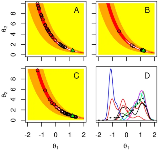
3.1 Results for the simulation study of the toy example. A. IF1 point estimates from 30 replications (circles) and the MLE (green triangle). The region of parameter space with likelihood within 3 log units of the maximum (white), with 10 log units (red), within 100 log units (orange) and lower (yellow). B. IF2 point estimates from 30 repli-cations (circles) with the same algorithmic settings as IF1. C. Final parameter value of 30 PMCMC chains (circles). D. kernel density estimates of the posterior for θ1 for the first 8 of these 30 PMCMC chains (solid lines), with the true posterior distribution (dotted black line). . . 34 3.2 Comparison of IF1 and IF2 on the cholera model. Points are the

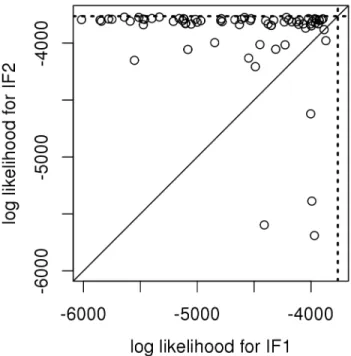
log likelihood of the parameter vector output by IF1 and IF2, both started at a uniform draw from a large hyper-rectangle (see A.10). Likelihoods were evaluated as the median of 10 particle filter replica-tions (i.e., IF applied with M = 1 and σ1 = 0) each withJ = 2×104 particles. 17 poorly performing searches are off the scale of this plot (15 due to the IF1 estimate, 2 due to the IF2 estimate). Dotted lines show the maximum log likelihood reported by King et al. (2008). . . 37 4.1 Comparison of estimators for the linear, Gaussian toy example,

show-ing the densities of the MLEs estimated by the IF1, IF2, IS1, RIS1, and IS2 methods. The parametersα2 andα3 were estimated, started from 200 randomly uniform initial values over a large rectangular region [−1,1]×[−1,1]. MLE is shown as a dashed vertical line. . . 59 4.2 The density of the maximized log likelihood approximations

esti-mated by IF1, IF2, IS2 and RIS1 for the malaria model when using

J = 1000 and M = 50. The log likelihood at a previously computed MLE is shown as a dashed vertical line. . . 63

(9)

4.3 The density of the maximized log likelihood approximations esti-mated by IF1, IF2 and IS2 for the malaria model when using J = 10000 and M = 100 . . . 64 5.1 A compartment model of malaria transmission. . . 85 5.2 Monthly reportedP falciparum malaria cases (solid line) and monthly

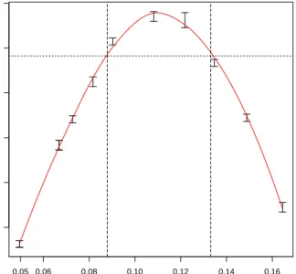
rainfall from a local weather station (broken line) for Kheda. . . 90 5.3 Profile likelihood plot for the control (bc) for the SEIQS model with

rainfall. The profile is estimated via fitting a smooth curve through Monte Carlo evaluations shown as confidence interval segment SEIQS. 95 5.4 Profile likelihood plot for the mean development delay time of mosquitoes

(τ) for the SEIQS model with rainfall. . . 95 5.5 Comparison between IF1 and IF2. . . 96 6.1 Simulated data from the Gompertz model (6.9, 6.10). This figure

shows the result of executing plot(gompertz, variables = ”Y”). . . 119 6.2 Convergence plots can be used to help diagnose convergence of the

iterated filtering (IF) algorithm. These and additional diagnostic plots are produced when plot is applied to a mif or mifList object. 123 6.3 Diagnostic plots for the PMCMC algorithm. The trace plots in the

left column show the evolution of 5 independent MCMC chains af-ter a burn-in period of length 20000. Kernel density estimates of the marginal posterior distributions are shown at right. The effec-tive sample size of the 5 MCMC chains combined is lowest for the

r variable and is 180: the use of 40000 proposal steps in this case is a modest number. The density plots at right show the estimated marginal posterior distributions. The vertical line corresponds to the true value of each parameter. . . 125 6.4 Results of plot on a probed.pomp-class object. Above the diagonal,

the pairwise scatterplots show the values of the probes on each of 1000 data sets. The red lines show the values of each of the probes on the data. The panels along the diagonal show the distributions of the probes on the simulated data, together with their values on the data and a two-sided p value. The numbers below the diagonal are the Pearson correlations between the corresponding pairs of probes. 131

(10)

6.5 Marginal posterior distributions using full information via pmcmc (solid line) and partial information via abc (dashed line). Kernel density estimates are shown for the posterior marginal densities of log₁₀(r) (left panel), log₁₀(σ) (middle panel), and log₁₀(τ) (right panel). The vertical lines indicate the true values of each parameter. . . . 133 6.6 Comparison of mif and nlf for 10 simulated datasets using two

cri-teria. In both plots, the maximum likelihood estimate (MLE), ˆθ, obtained using iterated filtering is compared with the maximum sim-ulated quasi-likelihood (MSQL) estimate, ˜θ, obtained using nonlinear forecasting. (A) Improvement in estimated log likelihood, ˆ`, at point estimate over that at the true parameter value, θ. (B) Improvement in simulated log quasi-likelihood ˆ`Q, at point estimate over that at

the true parameter value, θ. In both panels, the diagonal line is the 1-1 line. . . 135 6.7 Diagram of the SIR epidemic model. The host population is divided

into three classes according to infection status: S, susceptible hosts; I, infected (and infectious) hosts; R, recovered and immune hosts. Births result in new susceptibles and all individuals have a common death rateµ. Since the birth rate equals the death rate, the expected population size, P =S+I+R, remains constant. The S→I rate, λ, called the force of infection, depends on the number of infectious in-dividuals according toλ(t) =β I/N. The I→R, or recovery, rate isγ. The case reports,C, result from a process by which new infections are recorded with probability ρ. Since diagnosed cases are treated with bed-rest and hence removed, infections are counted upon transition to R. . . 136 6.8 Result of plot(sir1). The pomp object sir1 contains the SIR model

with simulated data. . . 144 6.9 One realization of the SIR model with seasonal contact rate,

im-ported infections, and extrademographic stochasticity in the force of infection. . . 155 A.1 PMCMC convergence assessment, using the diagnostic quantity in

equation A.21. (A) Underdispersed chains, all started at the MLE. (B) Overdispersed chains, started with draws from the prior (solid line), and underdispersed chains (dotted line). The average accep-tance probability was 0.04238, with Monte Carlo standard error 0.00072, calculated from iterations 5000 through 20000 for the 100 underdis-persed PMCMC chains. For the overdisunderdis-persed chains, the average acceptance probability was 0.04243 with standard error 0.00100. . . 167

(11)

A.2 The Liu & West algorithm Liu and West (2001) applied to the toy example with varying values of the discount factor: (A)δ= 0.99; (B)

δ = 0.999; (C) δ = 0.9999. Solid lines show 8 independent estimates of the marginal posterior density of θ1. The black dotted line shows the true posterior density. . . 170 A.3 Effective sample size (ESS) for SMC with fixed parameters and with

perturbed parameters. We ran SMC for the cholera model with the parameter vector set at the MLE, ˆθ, and at an alternative parameter vector ˜θ for which the first 18 parameters in Table 1 were multi-plied by a factor of 0.8. We defined the ESS at each time point by the reciprocal of the sum of squares of the normalized weights of the particles. The mean ESS was calculated as the average of these ESS values over the 600 time points. Repeating this computa-tion 100 times, using J = 104 particles, gave 100 mean ESS values shown in the “fixed” columns of the box-and-whisker plot. Repeat-ing the computation with additional parameter perturbations havRepeat-ing random walk standard deviation of 0.01 gave the 100 mean ESS val-ues shown in the “perturbed” column. For both parameter vectors, the perturbations greatly increase the spread of the mean ESS. At ˆθ, the perturbations decreased the mean ESS value by 5% on average, whereas at ˜θthe perturbations increased the mean ESS value by 13% on average. The MLE may be expected to be a favorable parameter value for stable filtering, and our interpretation is that the parameter perturbations have some chance of moving the SMC particles away from this favorable region. When started away from the MLE, the numerical stability of the IF2 algorithm benefits from the converse effect that the parameter perturbations will move the SMC particles preferentially toward this favorable region. For parameter values even further from the MLE than ˜θ, SMC may fail numerically for a fixed parameter value yet be feasible with perturbed parameters. . . 173 A.4 Comparison of different estimators. The likelihood surface for the

linear, Gaussian model, with likelihood within 2 log units of the maximum shown in red, within 4 log units in orange, within 10 log units in yellow, and lower in light yellow. The location of the MLE is marked with a green cross. The black crosses show final points from 40 Monte Carlo replications of the estimators: (A) IF1 method; (B) IF2 method; (C) IS2 method; (D) RIS1 method. Each method, except RIS1, was started uniformly over the rectangle shown, with

M = 25 iterations, N = 1000 particles, and a random walk stan-dard deviation decreasing from 0.02 geometrically to 0.011 for both

α2 andα3. We use bigger random walk standard deviations for RIS1. Specifically random walk standard deviations decrease from 0.23 ge-ometrically to 0.125 for both α2 and α3. . . 190

(12)

A.5 The distributions of likelihoods corresponding to Monte Carlo MLE approximations estimated by IF1, IF2, RIS1 and IS2 methods for toy model. The MLE is shown as a dashed vertical line (dark blue in elec-tronic version). The optimizations were started from 200 randomly uniform initial values over a rectangle. . . 191

(13)

LIST OF TABLES

Table

4.1 Summary of algorithms in iterated filtering/smoothing class . . . . 57 4.2 Computation times, in seconds, for the toy example. . . 59 5.1 A likelihood-based comparison of the fitted models. AIC is defined

as −2`+ 2p. . . 92 5.2 List of symbols used in the article with a description and units. . . . 92 6.1 Constituent methods for pomp objects and their translation into

mathematical notation for POMP models. For example, the rprocess method is set using the rprocess argument to the pomp constructor function. . . 102 6.2 Inference methods for POMP models. For those currently

imple-mented in pomp, function name and a reference for description are provided in parentheses. Standard Expectation-Maximization (EM) and Markov chain Monte Carlo (MCMC) algorithms are not plug-and-play since they require evaluation of fXn|Xn−1(xn|xn−1;θ). The

Kalman filter and extended Kalman filter are not plug-and-play since they cannot be implemented based on a model simulator. The Kalman filter provides the likelihood for a linear, Gaussian model. The ex-tended Kalman filter employs a local linear Gaussian approxima-tion which can be used for frequentist inference (via maximizaapproxima-tion of the resulting quasi-likelihood) or approximate Bayesian inference (by adding the parameters to the state vector). The Yule-Walker equations for ARMA models provide an example of a closed-form method of moments estimator. . . 105

(14)

6.3 Results of estimating parametersr,σ, andτ of the Gompertz model (6.9,6.10) by maximum likelihood using iterated filtering (4), com-pared with the exact MLE and with the true value of the parameter. The first three columns show the estimated values of the three pa-rameters. The next two columns show the log likelihood, ˆ`, estimated by SMC (2) and its standard error, respectively. The exact log likeli-hood, `, is shown in the rightmost column. An ideal likelihood-ratio 95% confidence set, not usually computationally available, includes all parameters having likelihood within qchisq(0.95,df=3)/2 = 3.91 of the exact MLE. We see that both the mif MLE and the truth are in this set. In this example, the mif MLE is close to the exact MLE, so it is reasonable to expect that profile likelihood confidence inter-vals and likelihood ratio tests constructed using the mif MLE have statistical properties similar to those based on the exact MLE. . . . 150 6.4 Parameter estimation by means of maximum synthetic likelihood (6)

vs. by means of maximum likelihood via iterated filtering (4). The row labeled “guess” contains the point at which both algorithms were initialized. That labeled “truth” contains the true parameter value, i.e., that at which the data were generated. The rows labeled “MLE” and “MSLE” show the estimates obtained using iterated filtering and maximum synthetic likelihood, respectively. Parameters r, σ, and

τ were estimated; all others were held at their true values. The columns labeled ˆ` and ˆ`_S are the Monte Carlo estimates of the log likelihood and the log synthetic likelihood, respectively; their Monte Carlo standard errors are also shown. While likelihood maximization results in an estimate for which both ˆ` and ˆ`_S exceed their values at the truth, the value of ˆ`at the MSLE is smaller than at the truth, an indication of the relative statistical inefficiency of maximum synthetic likelihood. . . 150

(15)

ABSTRACT

Iterated Filtering and Smoothing with Application to Infectious Disease Models by

Dao X. Nguyen

Chair: Edward L. Ionides

Partially observed Markov process (POMP) models are ubiquitous tools for model-ing time series data in many fields includmodel-ing statistics, econometrics, ecology, and engineering. Because of incomplete measurements, and possibly weakly identifiable parameters, making inferences on POMP models can be challenging. Standard meth-ods for inference (e.g., maximum likelihood) with restrictive assumptions of linear Gaussian models have often led to unsatisfactory results when the assumptions are violated. To relax these assumptions, this dissertation develops a class of simulation-based algorithms called iterated filtering and smoothing for POMP models. First, a novel filter, called Bayes map iterated filtering, is introduced. This filter recursively combines parameter perturbations with latent variable reconstruction, stochastically optimizing the approximated likelihood of latent variable models and providing an assymptotic guarantee of the performance of this inference methodology. Second, a fast, light-weight algorithm, called second-order iterated smoothing is proposed to im-prove on the convergence rate of the approach. The goal of this part is to demonstrate that by exploiting Fisher Information as a by-product of the inference methodology, one can theoretically achieve both statistical and computational efficiencies without

(16)

sacrificing applicability to a general class of models. Third, a new technique for the proof of Bayes map iterated filtering algorithm, based on super-martingale in-equality, is proposed. This approach with verifiable conditions is simpler than the previous approach and is generalizable to more sophisticated algorithms. Fourth, we validated the properties of the proposed methodologies through applying them to a challenging inference problem of fitting a malaria transmission model with control to time series data, finding substantial gains for our methods over current alterna-tives. Finally, a range of modern statistical methodologies for POMP modeling have been implemented in an open source R package, named pomp, to provide a flexible computational framework for the community.

(17)

CHAPTER I

Introduction

1.1 Motivation

Partially observed Markov process (POMP) models, which are synonymous with hidden Markov models or state space models, are defined as a doubly stochastic pro-cess where the underlying stochastic propro-cess can only be observed through another stochastic process (Rabiner and Juang, 1986). The past decade has seen the rapid development of POMP modeling in many fields including engineering, ecology and statistics. The reason could be that POMP modeling is especially appealing mecha-nisms for inference because most data are partially observable in nature. However, POMP modeling is hindered by the possibility of weak identifiability, which is often plagued by incomplete or noisy measurements. Thus, except when applied to cer-tain relative small, or approximately linear and Gaussian, state-of-the-art statistical methods are needed to make efficient use of available data and to facilitate model criticism.

Inference methodology for stochastic dynamic systems is often termed “plug-and-play” if only simulated estimation is needed to plug into the inference procedure (Bret´o et al., 2009; He et al., 2010). The plug-and-play methodology has been used to free researchers from demanding closed-form expression requirements for transi-tion probabilities, imposed by previously available statistical methodology, allowing

(18)

researchers to broaden classes of modeling and considering novel hypotheses. Un-like the mainstream statistical techniques (Expectation-Maximization algorithms and Bayesian Markov Chain Monte Carlo), plug-and-play approaches are a relatively re-cent and exciting development because of their less restrictive requirements. Examples of plug-and-play methodologies follow the frequentist paradigm (Ionides et al., 2011; Lindstr¨om et al., 2012), the Bayesian paradigm (Andrieu et al., 2010; Toni et al., 2009), or work by matching selected summary statistics (Wood, 2010). Amongst these approaches, we are interested in iterated filtering, a frequentist plug and play method that applies a sequence of standard sequential Monte Carlo (SMC) filter-ing algorithms to recursively locate the maximum likelihood estimator of unknown system parameters. The reason is that likelihood maximization provides a general platform for hypothesis testing, interval estimation, and diagnosis of model misspecifi-cation. By making likelihood maximization computationally feasible for increasingly large systems, iterated filtering has provided computational savings. The method-ological difficulties carrying out inference for partially observed stochastic dynamic system models are primarily computational. Although, the fundamental theories of likelihood-based or Bayesian inference are generally applicable to POMP, at least in principle, they aren’t frequently used because of their computational costs. A mod-ern and popular fully-Bayesian plug-and-play sequential Monte Carlo based method, (Andrieu et al., 2010) considers only a single value of the model parameter vector at each of the numerically intensive integration steps, which imposes considerable com-putational cost. By contrast, iterated filtering obtains massive comcom-putational savings over alternative Monte Carlo methodologies by searching the model parameter space simultaneously with integrating out over latent dynamic state variables.

It is well-known that iterated filtering theory is based on stochastic approxima-tion, for which the convergence rate is suboptimal. It is desirable to increase the convergence rate of this class of algorithms to enlarge the applicability in real-world

(19)

problems. Therefore, it is essential to improve the convergence rate of this class of inference algorithms while enjoying its advantages.

1.2 Contribution

There are several key contributions. The first contribution is a novel theoretical framework for a Bayes map iterated filtering and a new algorithm construction that dramatically outperforms previous approaches on a challenging inference problem in disease ecology. In order to increase empirical convergence rate for Bayes map iterated filtering, we generalize the idea of data cloning (Lele et al., 2007) and the classical iterated filtering (Ionides et al., 2011). While the core description of the iterated filtering is based on conditional moments of the perturbed parameters to approximate derivatives of the log-likelihood function, the proof of this method is particularly dealing with convergence of an iterated Bayes map. Specifically, it has been shown that if we apply Bayes map iteratively, we finally get a good approximation of the maximum likelihood. From a practical point of view, we find this new algorithm can lead to substantial numerical improvements in the process of inferring parameters of a POMP model. Methods that are not based on local polynomial approximations to the likelihood surface can be advantageous when the likelihood surface has nonlinear ridges, a situation that is highlighted by both the toy example and the scientific example in the manuscript.

The second contribution is the use of more natural random walk noise instead of independent white noise in the framework of iterated smoothing (Doucet et al., 2013). The focus in this part is on presenting how to improve empirical convergence rate without increasing computational work load. It is an open problem whether the approach proposed by Doucet et al. can be applied in practice, while we find a the-oretical simplification, which leads directly to a computationally simpler algorithm. Furthermore, it can be shown that this Taylor-series based algorithm remains

(20)

com-petitive with the iterated Bayes map approach. This approach therefore provides an alternative platform for potential future theoretical and practical progress on tackling this class of inference problems. Based theoretically on proofs ofDoucet et al.(2013), we introduce a theoretical development that our empirical results suggest is critical for turning the insights into a computationally efficient algorithm. We present evidences for the computational capabilities of our algorithm on challenging scientific problems. By contrast, (Doucet et al., 2013), to the best of our knowledge, did not demonstrate practical applications for their algorithm. In addition, we try to implement Doucet et al.’s algorithm and its variation closest to their theory and compare performances amongst different approaches. The comparison confirms that the random walk noise approach explores the likelihood surface more efficiently than the independent white noise approaches, a situation that is illustrated by both the toy and the scientific examples.

The third contribution is the use of super martingale theory, to prove the conver-gence of Bayes map iterated filtering. Using this general proof technique, which only relies on easily verifiable conditions, is of general interest. Such approaches, are sim-ple, elegant and generalizable to more sophisticated algorithms. We also apply it to a more challenging data analysis, difficult to analyze before. Hence, we demonstrate it as a viable method for some challenging models, including causal inference system under reactive intervention, which severely violate the conditional independence of POMP model. In order to avoid conditional independence violation, we propose to use proper weight for a SMC proposal density. We verify the performance improve-ment of the method on a toy problem of stochastic volatility with return. The results confirm our previous finding that Bayes map iterated filtering is an effective plug and play approach and it is applicable in the new modeling framework.

Finally, in order to evaluate these proposed algorithms, extensive experiments have been conducted successfully on an infectious diseases datasets obtained from

(21)

Na-tional Institute of Malaria Research in India in collaboration with Mercedes Pascual. R package pomp (King et al., 2015c) is used as modeling framework and inference environment for general data analysis implementation. Various cluster and paralel-lization libraries are used for the proposed algorithms. Experimental results show that the proposed algorithms improve substantially the convergence rate for a given computational budget. Most importantly, it provides a scalable framework for POMP models to deal with most real world datasets. Some recent Bayesian approaches also try to exploit the plug and play properties, using computational power of paralleliza-tion, however, our method is believed to give a very potential application by using approximated maximum likelihood with much simpler computational expenses. At the end, a conclusion with some open issues and future work are presented.

Our contribution to the statistical communities includes:

1. Iterated Bayes map filtering with better convergence rate and less computational time.

2. A light-weight second-order iterated smoothing with competitive computational performance.

3. A new elegant generalizable proof of Bayes map iterated filtering. 4. Contributing to open source R packages pomp.

5. Develop open source R packages, is2.

6. Scientific data analysis of models with feedback controls with application to malaria with controls datasets.

1.3 Overview of the dissertation

(22)

Chapter 1 gives motivation, objectives and contributions of the dissertation. Chapter 2 introduces a background of partially observed Markov model. The stochastic approximation, sequential Monte Carlo approximation of the likelihood and original iterated filtering with some brief mathematical formalizations of the conventional framework. This constitutes the theoretical foundations of the disserta-tion.

Chapter 3, presents a novel Bayes map iterated filtering, which is capable of improving convergence rate of the simulation-based inference approach by iteratively combine parameter perturbations with latent variable reconstruction.

Chapter 4 then focuses on developing a novel theoretical justification for the second order iterated smoothing algorithm. The main theoretical results show that we can approximate the first and the second-order derivative of the log-likelihood function using conditional moments. The approach ofDoucet et al. (2013) can be modified to construct an algorithm which carries out smoothing using random walk perturbations, with the happy result that some computationally demanding covariance terms cancel out and do not have to be computed.

Chapter 5 first reprove Bayes map iterated filtering using supermartingale theory. It then proposes a framework for inference on mechanistic model, accounting for control effects. The chapter includes the carried out experiments. The results are carefully analyzed and discussed in details. It concludes at the end with open issues and future works.

Chapter 6 provide a software environment that can effectively handle broad classes of POMP models and take advantage of the wide range of statistical methodologies that have been proposed for such models. The pomp software package (King et al., 2015c) differs from previous approaches by providing a general and abstract repre-sentation of a POMP model. The chapter also illustrates the specification of more complex POMP models, using a nonlinear epidemiological model with a discrete

(23)

population, seasonality, and extra-demographic stochasticity. It discusses the specifi-cation of user-defined models and the development of additional methods within the programming environment provided by pomp.

(24)

CHAPTER II

Background on Iterated Filtering Algorithms

2.1 Partially Observed Markov Model

We use capital letters to denote random variables and lower case letters to de-note their values. Let {X(t), t ∈ _T} be a Markov process with X(t) taking values in a measurable space X. The time index set, _T ⊂ _R, may be an interval or a discrete set and contains a finite subset t1 < t2 < · · · < tN at which X(t) is

ob-served, together with some initial time t0 < t1. We write X0:N = (X0, . . . , XN) =

(X(t0), . . . , X(tN)). Hereafter for any generic sequence {Xn}, we shall use Xi:j to

denote (Xi, Xi+1, . . . , Xj). The distribution of X0:N is characterized by the

ini-tial density X0 ∼ µ(x0;θ) and the condition density of Xn given Xn−1, written as

fn(xn|xn−1;θ) for 1≤ n ≤N. Here, θ is an unknown parameter in Rd. The process

{Xn} is only observed through another process{Yn, n= 1, . . . , N}taking values in a

measurable space Y. The observations are assumed to be conditionally independent given {Xn}, and their probability density is of the form

pYn|Y1:n−1, X0:n(yn|y1:n−1, x0:n;θ) =gn(yn|xn;θ),

for 1≤n≤N. We assume thatX0:N and Y1:N have a joint densitypX0:N, Y1:N(x0:N, y1:N;θ)

onXN+1_×YN_{. The data are a sequence of observations by}_y∗

1:N = (y

∗

1, . . . , y ∗

(25)

considered as fixed. We write the log likelihood function of the data for the POMP model as `(θ), given by `(θ) = logpY1:N(y ∗ 1:N;θ) = log Z µ(x0;θ) N Y n=1 fn(xn|xn−1;θ) gn(yn∗|xn;θ) dx0:N.

2.2 Stochastic Approximation

Stochastic approximation, first introduced in 1951 by Robbins and Monro (1951), has been subject to enormous literature, including statistical computation. The stochastic approximation ofRobbins and Monro procedure is to find zeros of function

g(x), which can only be computed through noisy observations. The basic paradigm is a stochastic difference equation of the form θn+1 = θn+nYn, where θn takes its

values in some Euclidean space, Yn is a random variable. The “step size” n > 0

is small and might go to zero as n → ∞. The parameter θ is to be estimated to meet a goal asymptotically given that the random vector Yn is a noise-corrupted

ob-servations sequence taken on the system when the parameter is set to θn. A major

insight of Robbins and Monro was that, if the step sizes n goes to zero slow enough

asn→ ∞, then noise will be canceled out in the long run through implicit averaging of the observation. The Robbins Monro algorithm is essentially a recursive proce-dure for finding the root of a real value function g(·). It turns out to be a classical one in numerical analysis and Newton’s procedure if g(·) is known and continuously differentiable. The sequence θn is computed recursively as

θn+1 =θn−[g0(θn)]−1g(θn), n= 1,2, ... (2.1)

where g0(·) denotes the derivative of g(·) with respect to θ. Suppose that g(θ) < 0 forθ > θ∗, and g(θ)>0 forθ < θ∗, and that g0(θ) is strictly negative and is bounded

(26)

in a neighborhood of θ∗. Then θn converges toθ∗ if the initial value θ1 is in a small enough neighborhood of θ∗. In general, g(·) is neither differentiable nor known, the estimation is often replaced by a good approximation approach such as Monte-Carlo estimation. If the goal is to stochastically estimate the maximum of a function g(θ) whereθ isddimensional parameter. It is equivalent to finding the zeros points of the gradient ∇g(θ) or Kiefer and Wolfowitz (1952)(KW) method. Let cn → 0 denote

the finite difference width used for gradient approximation, n denote the step size

and Yn,i denote the observation taken at time n at parameter value θn along the ith

unit vector direction ei. We define θn recursively by

θn+1 =θn+nYn, (2.2) where Yn= (Yn,1, ..., Yn,d) and Yn,i= g(θn+cnei)−g(θn−cnei) 2cn . (2.3)

Additional difficulties arise due to bias in estimating ∇g(θ). Let g_i0(θ), g_i00(θ),g_i000(θ) denote the first, second and third derivative ofg with respect to ith component ofθ. Suppose g_i000(θ) are continuous. By a Taylor expansion,

gθˆn+cnei =gθˆn +cngi0 ˆ θn +1 2c 2 ng 00 i ˆ θn +1 6c 3 ng 000 i θ¯n(i+) , (2.4) gθˆn−cnei =gθˆn −cngi0 ˆ θn + 1 2c 2 ng 00 i ˆ θn − 1 6c 3 ng 000 i θ¯ (i−) n , (2.5)

where ¯θ(ni±) = ˆθn+λ±cnei for some λ± ∈ [0,1]. Assume that the difference of noise

term in any direction has a conditional mean zero, then by some calculation

EhYn,i|θˆ0, ...,θˆn

i

=g0_iθˆn

(27)

where bn,i is the ith term of the bias. Assume that gi000

¯

θ(ni±)

are bounded, this implies the bias bn,i =O(c2n). The algorithm converges if bn → 0. For example, if g

is a quadratic loss function, it always holds.

2.3 Adaptive Stochastic Approximation

Stochastic approximation approach is in a sense a stochastic generalization of the gradient descent method. As a result, it is often possible to improve the speed of con-vergence by stochastic generalization of Newton method using Hessian of the objective functions. It is stated that this can lead to an asymptotically optimal convergence rate (Gill et al., 1981). However, the computation of Hessian by supplying second deriva-tive and matrix inversion is burdensome, Quasi-Newton methods can replace this by simpler updating formula (Fletcher, 1980). Suppose that the objective function is to minimize r(x) = kg(x)k2 = Pd

i=1gi2(x) where g(x) = (g1(x), ..., gd(x)), x ∈

Rd_{, n}_≥_d_{. Let} _D₍_x_{) be the}_d_×_d _{derivative of} _g₍_x_{). Then the derivative of}_k_g₍_x_)k2

is 2DT(x)g(x). The Hessian matrix of kg(x)k2 is

H(x) = 2 " DT (x)D(x) + d X i=1 H(i)(x)gi(x) # , (2.7)

wheregi isith coordinate of g andH(i) is the Hessian ofgi. Thus one can by pass the

expensive computation of Hessian either by general quasi Newton method (Fletcher, 1980) or by Gauss-Newton method which exploit the special structure of r(x).

∇2_r₍_x_{) = 2} n X i=1 h (∇gi(x)) (∇gi(x))T + ∇2gi(x) gi(x) i , (2.8)

and since fi(x)≈0 is near the minimum of r(x),

∇2_r₍_x₎_≈₂

n

X

i=1

(28)

Note that ∇r(x) = 2DT ₍_x₎_g₍_x_{) where} _DT ₍_x_{) = (∇}_f

1(x), ...,∇fn(x)). The

Gauss-Newton recursion is

xn+1 =xn−[DT (xn)D(xn)]−1DT (x)g(x). (2.10)

D(xn) is assumed to have rank k, when n=k,D(x)is invertible and

[DT (xn)D(xn)]−1DT (x) =D−1(x). (2.11)

Hence, adaptive stochastic approximation can be a simple form of

xn+1 =xn−D−1(x)g(x). (2.12)

In the context of parameter estimation, exploiting the structure of iterated filtering, the Hessian can be by passed for free, while the optimal convergence rate of adaptive stochastic approximation can be achieved.

2.4 Data Cloning

The data cloning method (Lele et al., 2007) can briefly described as follows. Con-sider the latent variable model X ∼ f(x|θ) with θ ∈Θ, where Θ = Rd _{denoted the}

parameter space. Let y∼g y|θ be the observation model. We have the likelihood

L(θ, y) =

Z

g y|X, θf(X|θ)dX, (2.13)

and we want to compute the MLE. Let `(θ) = log L(θ),

θ∗ = arg max

θ∈Θ

(29)

Let π(θ) be the prior distribution on the parameter space Θ, using the posterior distribution πn θ|y = g y|θnπ(θ) R g y|θnπ(θ)dθ. (2.15)

The authors show that under some regularities, if θn∼πn, then

θn P →θ∗, √ nΣ (θn−θ∗)⇒N(0, Id), where Σ=4 {−∇2_`₍_ϑ₎_| ϑ=θ∗} −1/2

. The precise statement is as follows.

Assumption II.1. g(·) as a function of θ has a local maximum at θ∗, g(θ∗) > 0,

π(θ∗)>0.

Assumption II.2. π is continuous at θ∗, g(·) is of class C2 _{in a neighborhood of}

θ∗and H(θ) =∇2_g₍_θ_∗) _{is strictly negative definite.}

Assumption II.3. For any δ >0, γ(δ) := sup{g(θ) :kθ−θ∗k> δ}< g(θ∗). Theorem II.4. Lele et al. (2010) Assume Assumptions A.1 - II.3. Setψn

4

=√nΣ (θn−θ∗).

As n → ∞, θn converges in probability to θ∗ and ψn converges weakly to N(0, Id).

Definition II.5. (Neighborhood). Letδ >0,defineN(δ) := {θ:kΣ−1₍_θ₋_θ_∗)k_{< δ}_}_.

Definition II.6. Let θn ∈ Rd with density function πn(·), define the standardized

variable ψn =

√

nΣ−1(θn−θ∗) that has the density gn(θ) =

|Σ| nd/2πn θ∗+√1_nΣθ . Lemma II.7. Assume Assumptions A.1 and A.2, for all θ∈Θ,

lim n→∞ g θ∗+ 1 √ nΣθ n = exp − kθk2/2 (2.16)

(30)

Proof. Fix δ0 so small that ∇2g(θ)is continuous in the neighborhood N(δ0). We assume without lost of generality thatg(θ∗) = 1, using Taylor expansion,∃θ+ ∈(θ, θ∗) such that g(θ) =g(θ∗) +∇g(θ∗) (θ−θ∗) + 1 2(θ−θ∗) T −∇2g(θ+) (θ−θ∗) = 1− 1 2(θ−θ∗) T −∇2_g₍_θ +) (θ−θ∗). (2.17) It is justified as ∇g(θ∗) = 0 and for any n large enough, θ∗+ √1_nΣθ is in N(δ0), so

g θ∗+ 1 √ nΣθ = 1− θ T_ΣT _{−∇2_g₍_θ n)}Σθ 2n , (2.18)

for some θn in the line segment

θ∗, θ∗+ √1_nΣθ

. For ε > 0, choose δ(ε) < δ0 small enough such that for θ ∈ N(δ(ε)), we have ∇2_g₍_θ_{) is negative definite and}

ΣT∇2g(θ) Σ−I

< ε. Then for 0≤x, y ≤n, we have 1− x n n −1− y n n ≤ |x−y|, and 1− y n n −exp (−y) ≤ y2 n. (2.19)

Fix M >1 and 0< ε <1 and let n >max (M/δ(ε))2, M2

. Then for kθk< M we haveθn ∈N(δ(ε)), so using (2.19) with x= 1₂θTΣT {−∇2g(θn)}Σθ and y=kθk2/2

we get g θ∗+ 1 √ nΣθ n −exp − kθk2/2 < εM 2 2 + M4 4n , (2.20)

(31)

Remark II.8. As π is continuous at θ∗, from the above Lemma II.7, π θ∗+ 1 √ nΣθ g θ∗ + 1 √ nΣθ n

converges to π(θ∗) exp − kθk2/2 uniformly on compact sets.

Remark II.9. Lemma II.7 and Fatou’s Lemma giveπ(θ∗)|Σ|(2π)d/2 ≤lim infnc(n)nd/2,

specifically there is a constant C >0 such that _c₍1_n₎ ≤Cnd/2

Lemma II.10. Assume Assumptions A.1 and A.2, the following are equivalent. (a) ψn⇒N(0, Id)

(b) gn converges point-wise to a multivariate standard normal density function, i.e

c(n)nd/2 _→_π₍_θ_∗)_|Σ|₍₂_π₎d/2

(c) θn⇒δθ∗ where δθ∗ indicate a Dirac-delta mass distribution Proof. (a) implies (b). Since gn can be written as

gn(θ) = |Σ| c(n)nd/2π θ∗+ 1 √ nΣθ g θ∗+ 1 √ nΣθ n . (2.21)

LetB be the compact Borel set with positive measure. From (a) we have 1 (2π)d/2 Z B exp − kθk2/2dθ ≤lim n |Σ| c(n)nd/2 Z B π θ∗+ 1 √ nΣθ g θ∗ + 1 √ nΣθ n dθ.

Uniform convergence from Lemma II.7 gives

lim n Z B π θ∗+ 1 √ nΣθ g θ∗+ 1 √ nΣθ n dθ=π(θ∗) Z B exp − kθk2/2dθ. (2.22)

(32)

Hence, c(n)nd/2 _→_π₍_θ

∗)|Σ|(2π)d/2 as n→ ∞. From Lemma II.7:

gn(θ)→ 1 (2π)d/2 Z B exp − kθk2/2dθ, (2.23)

(b) implies (a) by Scheffe’s theorem. (a) implies (c) is easy.

(c) implies (b). Since∇2_g _and_π_{are continuous at}_θ

∗and Σ is strictly positive definite, from Lemma II.7 we see that for any ε >0, we can find δ >0 so that θ ∈N(δ) and

g(θ)<1−1

2(1−ε) (θ−θ∗)

T

Σ−2(θ−θ∗), (2.24)

π(θ)≤π(θ∗) +ε.

From (c), we assume that n is large enough so 1−ε ≤ R

N(δ)πn(θ)dθ. Multiplying this inequality by c(n)nd/2(1−ε)−1and using (2.24) gives

c(n)nd/2 ≤(1−ε)−1nd/2 Z N(δ) π(θ)gn(θ)dθ ≤(1−ε)−1nd/2(π(θ∗) +ε)× Z N(δ) 1−1 2(1−ε) (θ−θ∗) T Σ−2(θ−θ∗) n dθ ≤(1−ε)−1nd/2(π(θ∗) +ε)× Z N(δ) exph1− n 2 (1−ε) (θ−θ∗) T Σ−2(θ−θ∗)idθ = (1−ε)−1nd/2(π(θ∗) +ε)|Σ|(2π)d/2. Letting n→ ∞ and ε→0, lim sup n c(n)nd/2 ≤π(θ∗)|Σ|(2π)d/2. (2.25)

(33)

Corollary II.11. Corollary to Lemma II.10. Assume Assumption A.1 - II.3, θn ⇒

δθ∗

Proof. From Assumption II.3 and Corollary II.11 to Lemma II.10, for any δ >0 1

c(n)

Z

kθ−θ∗k>δ

π(x)fn(x)dx≤Cnp/2γ(δ)n →0.

This implies θn⇒δθ∗ and

ψn ⇒N(0, Id).

The result of Theorem II.4 follows.

2.5 Sequential Monte Carlo

Sampling is one of the key concepts of sequential Monte Carlo approaches. Sam-pling techniques is a powerful resort whenever estimation statistics cannot be com-puted analytically. Most distribution are generated by using either analytical or approximative transformations of samples from a standard distribution. However, for distribution which is too complex to sample directly or by transformation, we must resort to other techniques, such as sampling importance resampling (SIR). Let

q be the importance distribution which is considerably easier to sample from and let

x(1)_{, x}(2)_{, . . . , x}(N) _{be a sample of size} _N _from _q_{. Sampling from} _q _{instead of} _p introduce importance weights ω˜(i)

˜

ω(i) =p(x(i))/q(x(i)), i= 1,2, . . . , N. (2.26)

Note that the more likely with respect to p the larger sample weight is. In that sense, re-sampling can be performed from these samples using sampling with

(34)

replace-ment, in which each sample x(i) _{has the probability of its normalized weight:} ω(i) = ω˜ (i) PN i=1ω˜(i) , i= 1,2, . . . , N. (2.27)

Thus a new sample ˜x(1),x˜(2), . . . , x˜(N) frompcan be drawn. By the Markov property of the distribution of interest, the sampling techniques can be carried out sequentially. Given the POMP structure of latent variables xt with initial distribution p0(x0), we can compute the weights recursively for each time step t. To sample the posterior distribution, importance distributionq0:t is chosen to satisfy:

q0:t(x0:t|y0:t) = q0:t−1(x0:t−1|y0:t−1)qt(xt|Xt−1, yt). (2.28)

The proportionality of importance weights are:

˜ ω_t(i) ∝ω˜(_t₋₁i) p(˜x (i) t |˜x (i) t−1)p(yt|˜x (i) t ) qt(˜x (i) t |˜x (i) t−1, yt) . (2.29)

A new sample of N particles from the previous sample is drawn according to the normalized weights and set the new weights to 1/N. Thus the outlined algorithm for each time step is as follows:

1. Sample ˜x(_ti) from qt(˜x (i) t |x (i),yt t−1 ). 2. Compute weights: ˜ω_t(i) =ω_t(−1i) p(˜x(_ti)|˜x_t(₋₁i) )p(yt|˜x (i) t ) qt(˜x (x) t 1˜x (x) t−1, yt) . 3. Normalize weights: ω(_ti) = ˜ω(_ti)/ N X j=1 ˜ ω_t(j).

(35)

2.6 Iterated Filtering

Iterated filtering for maximum likelihood inference was introduced inIonides et al. (2006), and later generalized to sequential Monte Carlo filters in Ionides et al.(2011).

The idea is to explore the parameter space by stochastic perturbation to smooth out the likelihood function. In the long run, the added noise will be canceled out through filtering while the parameter can be asymptotically achieved. The hidden {Xt}t∈N process is augmented by a time varying parameter process {Θ˘n}. Let K be

a density with compact support, zero mean and covariance matrix Σθ_{, and let} _ζ t be

an independent draw fromK. The time varying parameter process is then defined as

˘

Θ0 =θ+τ ζ0, (2.30)

˘

Θn= ˘Θn−1+σζn. (2.31)

The stochastically perturbed model is defined conditionally on the time varying pa-rameter process

g_X˘_0:_N_,_Y˘_1:_N_,_Θ˘_0:_N(x0:N, y1:N,θ˘0:N;θ, τ)

=fX0:N,Y1:N(x0:N, y1:N; ˘θ0:N)gΘ˘0N(˘θ0:N;θ, τ,Σ). (2.32)

Define the conditional mean and covariance

˘

θ_nF = Eθ,σ,τ[ ˘Θn|Y1:n =y1:n], (2.33)

˘

V_nP = Covθ,σ,τ[ ˘Θn|Y1:n−1 =y1:n−1]. (2.34) Ionides et al. (2011) shows that the score function can be approximated with these moments.

(36)

Theorem II.12. (Theorem 3 in Ionides et al. (2011) ). Let K1 be a compact subset of _Rp_{, C}

1 is a constant, τ is small enough and lim

τ→0σ(τ)/τ = 0. It then holds that

sup θ∈K1 | N X n=1 ( ˘V_nP)−1(˘θF_n −θ˘_nF₋₁)− ∇`N(θ)| ≤C1(τ+ σ2 τ2). (2.35) The framework is computationally attractive since moments are often easier to es-timate than gradients. In addition, an approximation of the log-likelihood is feasible through augmented filtered states. If the sequences {τm}, {σm} and {Jm} satisfied

theorem assumptions, ˜θF_n and ˜V_nP are conditional sample mean and covariance com-puted from a sequential Monte Carlo filter using Jm particles. It then follows from

Ionides et al. (2011) that

τmJm|EM C[( ˜Vn,mP ) −1 (˜θ_n,mF −θ˜_nF₋₁_,m)−( ˘V_n,mP )−1(˘θ_n,mF −θ˘_nF₋₁_,m)]| ≤C2, (2.36) and τ_m2JmVarM C[( ˜Vn,mP ) −1 (˜θF_n,m−θ˜_nF₋₁_,m)]≤C3. (2.37)

Theorem II.13. (Theorem 4 in Ionides et al. (2011) ). LetK2 be a compact subset of

Rd,{τm},{σm} and{Jm}be sequences such that τm →0, σmτm−1 →0andτmJm → ∞,

and define e ∇`N(θ) = N X n=1 ( ˜V_n,mP )−1(˜θ_n,mF −θ˜F_n₋₁_,m). (2.38) It then holds that

lim m→∞_θsup_∈_K 2 |EM C[∇e`_N(θ)]− ∇`_N(θ)|= 0, (2.39) lim m→∞_θsup_∈_K 2 |τ_m2JmVarM C[∇e`_N(θ)]|<∞. (2.40)

Theorem II.13 shows that the score function can be approximated arbitrarily well by decreasing the variances σ_m2, τ_n2 while simultaneously increasing the number of particles Jm. It can be used to define a difference equations for the parameter

(37)

estimates θm, by iteratively updating the estimates in the direction of the gradient

(steepest ascent method).

Theorem II.14. (Theorem 5 in Ionides et al. (2011) ). Let {γm}, {τm}, {σm} and

{Jm} be positive sequences such that τm →0, σmτm−1 →0, τmJm → ∞,

∞ X m=1 γm =∞ and ∞ X m=1

γ_m2J_m−1τ_m−2 <∞ and define θˆm according to:

ˆ θm+1 = ˆθm+γm N X n=1 ( ˜V_n,mP )−1(˜θ_n,mF −θ˜F_n₋₁_,m). (2.41)

The estimate will then converge to the M LE with probability one, θn a.s.

→ θ?_.

Choosing γm =m−1, τm2 =m−1, σm2 =m−(1+δ) and Jm =m(1/2+δ) where δ >0 is

(38)

CHAPTER III

Bayes Map Iterated Filtering

3.1 Introduction

Variations on the original iterated filtering algorithm have been proposed to extend it to general latent-variable models (Ionides et al., 2011) and to improve numerical performance (Doucet et al., 2013;Lindstr¨om et al., 2012). In this chapter, we study a new iterated filtering algorithm which generalizes the data cloning method (Lele et al., 2007, 2010) and is therefore also related to other Monte Carlo methods for likelihood-based inference (Doucet et al., 2002; Gaetan and Yao, 2003; Jacquier et al., 2007). Data cloning methodology is based on the observation that iterating a Bayes map converges to a point mass at the maximum likelihood estimate. Combining such iterations with perturbations of model parameters improves the numerical stability of data cloning and provides a foundation for stable algorithms in which the Bayes map is numerically approximated by sequential Monte Carlo computations.

We investigate convergence of a sequential Monte Carlo implementation of an iterated filtering algorithm which combines data cloning, in the sense of Lele et al (Lele et al., 2007), with the stochastic parameter perturbations used by the iterated filtering algorithm ofIonides et al. (2006). Lindstr¨om et al (Lindstr¨om et al., 2012) proposed a similar algorithm, termed fast iterated filtering, but the theoretical support for that algorithm involved unproved conjectures. We present convergence results for

(39)

our algorithm, which we call IF2. Empirically, it can dramatically out-perform the previous iterated filtering algorithm ofIonides et al.(2006), which we refer to as IF1. Though IF1 and IF2 both involve recursively filtering through the data, the theoretical justification and practical implementations of these algorithms are fundamentally different.

IF1 approximates the Fisher score function, whereas IF2 implements an iterated Bayes map. IF1 has been used in applications for which no other computationally fea-sible algorithm for statistically efficient, likelihood-based inference was known (King et al., 2008; Laneri et al., 2010; He et al., 2010; Blackwood et al., 2013a; Shrestha et al., 2013; Blake et al., 2014). The extra capabilities offered by IF2 open up further possibilities for drawing inferences about nonlinear partially observed stochastic dy-namic models from time series data. Iterated filtering algorithms implemented using basic sequential Monte Carlo techniques have the property that they do not need to evaluate the transition density of the latent Markov process. Algorithms with this property have been called plug-and-play (Bret´o et al., 2009;He et al., 2010). Various other plug-and-play methods for POMP models have been recently proposed (An-drieu et al., 2010; Toni et al., 2009; Wood, 2010; Shaman and Karspeck, 2012), due largely to the convenience of this property in scientific applications.

3.2 An algorithm and related questions

For a general POMP model defined as above, we look for a maximum likelihood estimate (MLE), i.e., a value ˆθ maximizing `(θ). The IF2 algorithm defined below provides

(40)

Algorithm IF2. Iterated filtering input: Simulator for fX0(x0;θ) Simulator for fXn|Xn−1(xn|xn−1;θ),n in 1 :N Evaluator for fYn|Xn(yn|xn;θ), n in 1 :N Data,y_1:∗_N Number of iterations, M Number of particles, J

Initial parameter swarm, {Θ0

j, j in 1 :J}

Perturbation density, hn(θ|ϕ;σ), n in 1 :N

Perturbation sequence, σ1:M

output: Final parameter swarm,{ΘM

j , j in 1 :J} Form in 1 :M Θ₀F,m_,j ∼h0(θ|Θjm−1;σm) forj in 1 :J ule[-2mm]0mm5mm X₀F,m_,j ∼fX0(x0; Θ F,m 0,j ) for j in 1 :J ule[-2mm]0mm5mm Forn in 1 :N ΘP,m_n,j ∼hn(θ|ΘF,mn−1,j, σm) for j in 1 :J ule[-2mm]0mm5mm X_n,jP,m ∼fXn|Xn−1(xn|X F,m n−1,j; Θ P,m j ) for j in 1 :J ule[-2mm]0mm5mm wm n,j =fYn|Xn(y ∗ n|X P,m n,j ; Θ P,m n,j ) for j in 1 :J ule[-2mm]0mm5mm

Draw k1:J with P(kj =i) =wmn,i

. PJ u=1w m n,u ΘF,m_n,j = ΘP,m_n,k j and X F,m n,j =X P,m n,kj for j in 1 :J ule[-2mm]0mm5mm End For Set Θm_j = ΘF,m_N,j for j in 1 :J End For

a plug-and-play Monte Carlo approach to obtaining ˆθ.

A simplification of IF2 arises when N = 1, in which case iterated filtering is called iterated importance sampling (Ionides et al., 2011) (see A.2). Algorithms

(41)

similar to IF2 with a single iteration (M = 1) have been proposed in the context of Bayesian inference (Kitagawa, 1998; Liu and West, 2001) (see A.6). When M = 1 and hn(θ|ϕ;σ) degenerates to a point mass at ϕ, the IF2 algorithm becomes

a standard particle filter (Arulampalam et al., 2002; Doucet et al., 2001). In the IF2 algorithm description, ΘF,m_n,j and X_n,jF,m are the jth particles at time n in the Monte Carlo representation of the mth iteration of a filtering recursion. The filtering recursion is coupled with a prediction recursion, represented by ΘP,m_n,j andX_n,jP,m. The resampling indices k1:J in IF2 are taken to be a multinomial draw for our theoretical

analysis, but systematic resampling is preferable in practice (Arulampalam et al., 2002). A natural choice of hn(θ|ϕ;σ) is a multivariate normal density with mean

ϕ and variance σ2_{Σ for some covariance matrix Σ, but in general} _h

n could be any

conditional density parameterized by σ. Combining the perturbations over all the time points, we define

h(θ0:N|ϕ;σ) =h0(θ0|ϕ;σ)

N

Y

n=1

hn(θn|θn−1;σ).

We define an extended likelihood function on ΘN+1 _by

˘ `(θ0:N) = Z . . . Z dx0. . . dxN n fX0(xo;θ0)× N Y n=1 fXn|Xn−1(xn|xn−1;θn)fYn|Xn(y ∗ n|xn;θn) o .

Each iteration of IF2 is a Monte Carlo approximation to a map

Tσf(θN) = R _˘ `(θ0:N)h(θ0:N|ϕ;σ)f(ϕ)dϕ dθ0:N−1 R _˘ `(θ0:N)h(θ0:N|ϕ;σ)f(ϕ)dϕ dθ0:N , (3.1)

with f and Tσf approximating the initial and final density of the parameter swarm.

For our theoretical analysis, we consider the case when the standard deviation of the parameter perturbations is held fixed at σm =σ >0 for m= 1, . . . , M.

(42)

In this case, IF2 is a Monte Carlo approximation to TM

σ f(θ). We call the fixed

σ version of IF2 homogeneous iterated filtering since each iteration implements the same map. For any fixed σ, one cannot expect a procedure such as IF2 to converge to a point mass at the MLE. However, for fixed but small σ, we show that IF2 does approximately maximize the likelihood, with an error that shrinks to zero in a limit asσ→0 andM → ∞. An immediate motivation for studying the homogeneous case is simplicity; it turns out that even with this simplifying assumption the theoretical analysis is not entirely straightforward. Moreover, the homogeneous analysis gives at least as much insight as an asymptotic analysis into the practical properties of IF2, when σm decreases down to some positive level σ > 0 but never completes the

asymptotic limitσm →0. Iterated filtering algorithms have been primarily developed

in the context of making progress on complex models for which successfully achieving and validating global likelihood optimization is challenging. In such situations, it is advisable to run multiple searches and continue each search up to the limits of available computation (Ingber, 1993).

If no single search can reliably locate the global maximum, a theory assuring convergence to a neighborhood of the maximum is as relevant as a theory assuring convergence to the maximum itself in a practically unattainable limit.

The map Tσ can be expressed as a composition of a parameter perturbation with

a Bayes map that multiplies by the likelihood and renormalizes. Iteration of the Bayes map alone has a central limit theorem (CLT) (Lele et al., 2007) which forms the theoretical basis for the data cloning methodology of Lele et al. (2007, 2010). Repetitions of the parameter perturbation may also be expected to follow a CLT.

One might therefore imagine that the composition of these two operations also has a Gaussian limit.

This is not generally true, since the rescaling involved in the perturbation CLT prevents the Bayes map CLT from applying (see A.4). Our agenda is to seek

(43)

condi-tions guaranteeing the following:

(A1) For every fixed σ >0, limm→∞Tσmf =fσ exists.

(A2) When J and M become large, IF2 numerically approximates fσ.

(A3) As the noise intensity becomes small, limσ→0fσ approaches a point mass at the

MLE, if it exists.

Stability of filtering problems and uniform convergence of sequential Monte Carlo nu-merical approximations are closely related, and so A1 and A2 are studied together in Theorem III.1. Each iteration of IF2 involves standard sequential Monte Carlo filter-ing techniques applied to an extended model where latent variable space is augmented to include a time-varying parameter.

Indeed, allM iterations together can be represented as a filtering problem for this extended POMP model on M replications of the data. The proof of Theorem III.1 therefore leans on existing results. The novel issue of A3 is then addressed in Theo-rem III.2.

3.3 Convergence of IF2

First, we follow the notations and proofs of Ionides et al. (2015). Let {Θ˘m_0:_N, m= 1,2, . . .} be a Markov chain taking values in ΘN+1 _{such that ˘}_Θ1

0:N has density

R

h(θ0:N|ϕ;σ)f(ϕ)dϕ, and ˘Θm0:N has conditional densityh(θ0:N|ϕN;σ) given ˘Θm0:N−1 =

ϕ0:N for m≥ 2. Suppose that{Θ˘m0:N, m ≥1} is constructed on the canonical

proba-bility space Ω ={(θ1

0:N, θ0:2N, . . .)} with θ0:mN = ˘Θm0:N(ϑ) forϑ = (θ0:1N, θ0:2N, . . .)∈Ω.

Let {Fm} be the corresponding Borel filtration. To consider a time-rescaled

limit of {Θ˘m_0:_N, m = 1,2, . . .} as σ → 0, let {Wσ(t), t ≥ 0} be a continuous-time,

right-continuous, piecewise constant process defined at its points of discontinuity by

(44)

filtered process defined such that, for any event E ∈ FM,

P_Z˘(E) =

E_Θ˘[˘`1:MIE]

E_Θ˘[˘`1:M]

, (3.2)

where IE is the indicator function for event E and

˘ `1:M(ϑ) = M Y m=1 ˘ `(θ_0:m_N).

In (3.2),_P_Z˘(E) denotes probability under the law of {Z˘nm}, andE_Θ˘ denotes expecta-tion under the law of{Θ˘m_n}. The process{Z˘_nm}is constructed so that ˘Z_Nm has density

Tm_f_{. We make the following assumptions.}

(B1) {Wσ(t),0≤t ≤1} converges weakly as σ→0 to a diffusion {W(t),0≤t≤1},

in the space of right-continuous functions with left limits equipped with the uniform convergence topology. For any open setA⊂Θ with positive Lebesgue measure and >0, there is a δ(A, )>0 such that_PW(t)∈A for all ≤ t≤ 1|W(0)

> δ.

(B2) For some t0(σ) and σ0 >0, Wσ(t) has a positive density on Θ, uniformly over

the distribution of W(0) for allt > t0 and σ < σ0.

(B3) `(θ) is continuous in a neighborhood{θ :`(θ)> λ1} for some λ1 <supϕ`(ϕ).

(B4) There is an > 0 with −1 > fYn|Xn(y

∗

n|xn, θ) > for all 1 ≤ n ≤ N, xn ∈ X

and θ ∈Θ.

(B5) There is a C1 such that hn(θ|ϕ;σ) = 0 when |θ−ϕ|> C1σ, for all σ.

(B6) There is a C2 such that sup1≤n≤N|θn−θn−1|< C1σ implies|`˘(θ0:N)−`(θN)|<

C2σ, for all σ and alln.

Conditions B1 and B2 hold when hn(θ|ϕ;σ) corresponds to a reflected Gaussian

random walk and {W(t)} is a reflected Brownian motion (see A.8). More generally,

(45)

will behave like Brownian motion in the interior of Θ. B4 follows if _X is compact and fYn|Xn(y

∗

n|xn;θ) is positive and continuous as a function ofθ and xn. B5 can be

guaranteed by construction. B3 and B6 are undemanding regularity conditions on the likelihood and extended likelihood.

A formalization of A1 and A2 can now be stated as follows.

Theorem III.1. Let Tσ be the map of (3.1) and suppose B2 and B4. There is a

unique probability density fσ such that for any probability density f on Θ,

lim

m→∞kT

m

σ f −fσk1 = 0, (3.3)

where kfk1 is the L1 norm of f. Let {ΘM

j , j = 1, . . . , J} be the output of IF2, with σm =σ >0. There is a finite

constant C >0 such that, for any function φ : Θ→_R and all M,

E 1 J J X j=1 φ(ΘM_j )− Z φ(θ)fσ(θ)dθ ≤ C sup_√θ|φ(θ)| J . (3.4)

Proof. B2 and B4 imply that Tk

σ is mixing, in the sense of Le Gland and Oudjane

(2004), for all sufficiently large k.

The results of Le Gland and Oudjane (2004) are based on the contractive proper-ties of mixing maps in the Hilbert projective metric. AlthoughLe Gland and Oudjane (2004) stated their results in the case whereT itself is mixing, the required geometric contraction in the Hilbert metric holds as long asTkis mixing for allK ≤k ≤2K−1 for some K ≥1 (Eveson, 1995, Theorem 2.5.1). Corollary 4.2 ofLe Gland and Oud-jane (2004) implies (3.3), noting the equivalence of the Hilbert projective metric and the total variation norm shown in their Lemma 3.4. Then, Corollary 5.12 ofLe Gland and Oudjane (2004) implies (3.4), completing the proof of Theorem III.1. A longer version of this proof is given in the supplement (see A.9).

(46)

Results similar to Theorem III.1 can be obtained using Dobrushin contraction tech-niques Del Moral and Doucet (2004). Results appropriate for non-compact spaces can be obtained using drift conditions on a potential functionWhiteley et al.(2012). Now we move on to our formalization of A3:

Theorem III.2. Assume B1–B6. For λ2 <supϕ`(ϕ),

limσ→0

R

fσ(θ)1{`(θ)<λ2}dθ = 0.

Proof. Let λ0 = supϕ`(ϕ) and λ3 = infϕ`(ϕ). From B4, ∞ > λ0 > λ3 > 0. For positive constants 1, 2, η1, η2 and λ1 < λ0, define

e1 = (1−1) log(λ0+2) +1log(λ2 +2),

e2 = (1−η1) log(λ1−η2) +η1log(λ3 −η2).

We can pick 1, 2, η1, η2 and λ1 so that e1 < e2. Suppose that {Θ˘mn} is initialized

with the stationary distributionf =fσ identified in Theorem III.1. Now, setM to be

the greatest integer less than 1/σ2, and letF1 be the event that{ΘmN, m= 1, . . . , M}

spends at least a fraction of time 1 in {θ:`(θ)< λ2}. Formally, F1 = n ϑ∈Ω : 1 M M X m=1 1{`(θm N)<λ2} > 1 o .

We wish to show that _P_Z˘[F1] is small for σ small. Let F2 be the set of sample paths that spend at least a fraction of time (1−η1) up to timeM in{θ :`(θ)> λ1}, i.e.,

F2 = n ϑ∈Ω : 1 M M X m=1 1{`(θm N)>λ1} >(1−η1) o .

(47)

Then, we calculate P_Z˘[F1] = E_Θ˘ _˘ `1:M1F1 E_Θ˘ _˘ `1:M ≤ EΘ˘ _˘ `1:M1F1 E_Θ˘ _˘ `1:M1F2 ≤ E ˘ Θ h QM m=1 `(θm N) +C2σ 1F1 i E_Θ˘ h QM m=1 `(θm N)−C2σ 1F2 i (3.5) ≤ EΘ˘ exp{M e1}1F1 E_Θ˘ exp{M e2}1F2 (3.6) = exp(e1−e2)M P ˘ Θ[F1] P_Θ˘[F2] . (3.7)

We used B5 and B6 to arrive at (3.5), then to get to (3.6) we have taken σ small enough that C2σ < 2 and C2σ < η2. From B3, {θ : `(θ) > λ1} is an open set, and B1 therefore ensures each of the probabilities _PΘ1:M[F1] and PΘ1:M[F2] in (3.7) tends

to a positive limit as σ → 0 given by the probability under the limiting distribution {W(t)} (see A.1). The term exp{(e1 −e2)M} tends to zero as σ → 0 since, by construction, M → ∞ and e1 < e2. Setting L = {θ : `(θ) ≤ λ2}, and noting that {Z˘m

N, m= 1,2, . . .} is constructed to have stationary marginal densityfσ, we have

Z L fσ(θ)dθ = 1 M M X m=1 n P_Z˘ _˘ Z_Nm ∈L|F1 P_Z˘[F1] + P_Z˘ _˘ Z_Nm ∈L|F₁c P_Z˘[F1c] o , ≤ 1+P_Z˘[F1],

which can be made arbitrarily small by picking1 small and σ small, completing the proof.

(48)

3.4 Demonstration of IF2 with nonconvex superlevel sets

Theorems 1 and 2 do not involve any Taylor series expansions, which are basic in the justification of IF1 (Ionides et al., 2011). This might suggest that IF2 can be effective on likelihood functions without good low-order polynomial approximations. In practice, this can be seen by comparing IF2 with IF1 on a simple two-dimensional toy example (dim(Θ) = dim(_X) = dim(_Y) = 2) in which the superlevel sets {θ :

`(θ) > λ} are connected but not convex. We also compare with particle Markov chain Monte Carlo (PMCMC) implemented as the PMMH algorithm ofAndrieu et al. (2010).

The justification of PMCMC also does not depend on Taylor series expansions, but PMCMC is computationally expensive compared to iterated filtering (Bhadra, 2010). Our toy example has a constant and non-random latent process, Xn =

exp{θ1}, θ2exp{θ1}

for n = 1, . . . , N. The known measurement model is

fYn|Xn(y|x;θ)∼Normal   x,    100 0 0 1      ,

This example was designed so that a nonlinear combination of the parameters is well identified whereas each parameter is marginally weakly identified. For the truth, we took θ = (1,1). We supposed that θ1 is suspected to fall in the interval [−2,2] and

θ2 is expected in [0,10]. We used a uniform distribution on this rectangle to specify the prior for PMCMC and to generate random starting points for all the algorithms. We set N = 100 observations, and we used a Monte Carlo sample size of J = 100 particles. For IF1 and IF2, we employed M = 100 filtering iterations, with initial random walk standard deviation 0.1 decreasing geometrically down to 0.01.