Multidatabase Interoperability
LAKS V. S. LAKSHMANAN The University of British Columbia FEREIDOON SADRI
University of North Carolina, Greensboro and
SUBBU N. SUBRAMANIAN Tavant Technologies
We provide a principled extension of SQL, called SchemaSQL, that offers the capability of uniform manipulation of data and schema in relational multidatabase systems. We develop a precise syntax and semantics ofSchemaSQLin a manner that extends traditional SQL syntax and semantics, and demonstrate the following. (1)SchemaSQL retains the flavor of SQL while supporting querying of both data and schema. (2) It can be used to transform data in a database in a structure substantially different from original database, in which data and schema may be interchanged. (3) It also permits the creation of views whose schema is dynamically dependent on the contents of the input instance. (4) While aggregation in SQL is restricted to values occurring in one column at a time,SchemaSQLpermits “horizontal” aggregation and even aggregation over more general “blocks” of information. (5)SchemaSQLprovides a useful facility for interoperability and data/schema manipulation in relational multidatabase systems. We provide many examples to illustrate our claims. We clearly spell out the formal semantics ofSchemaSQLthat accounts for all these features. We describe an architecture for the implementation ofSchemaSQLand develop implementation algorithms based on available database technology that allows for powerful integration of SQL based relational DBMS. We also discuss the applicability ofSchemaSQLfor handling semantic heterogeneity arising in a multidatabase system.
Categories and Subject Descriptors: H.2.3 [Database Management]: Languages—query lan-guages; H.2.4 [Database Management]: Systems—relational databases;query processing; H.2.5 [Database Management]: Heterogeneous Databases
L. V. S. Lakshmanan’s work was supported by a grant from the Natural Science and Engineering Research Council of Canada (NSERC).
F. Sadri’s work was supported by a grant from the National Science Foundation (NSF).
Authors’ addresses: L. V. S. Lakshmanan, Department of Computer Science, The University of British Columbia, 2366 Main Mall, Vancouver, BC V6T 1Z4, Canada, e-mail: [email protected]; F. Sadri, Department of Mathematical Sciences, University of North Carolina, Greensboro, NC 27410, e-mail: [email protected]; S. N. Subramanian, Tavant Technologies, 542 Lakeside Drive #5, Sunnyvale, CA 94085, e-mail: [email protected].
Permission to make digital or hard copies of part or all of this work for personal or classroom use is granted without fee provided that copies are not made or distributed for profit or direct commercial advantage and that copies show this notice on the first page or initial screen of a display along with the full citation. Copyrights for components of this worked owned by others than ACM must be honored. Abstracting with credit is permitted. To copy otherwise, to republish, to post on servers, to redistribute to lists, or to use any component of this work in other works requires prior specific permission and/or a fee. Permission may be requested from Publications Dept., ACM, Inc., 1515 Broadway, New York, NY 10036 USA, fax +1 (212) 869-0481, or [email protected].
C
General Terms: Algorithms, Languages
Additional Key Words and Phrases: Information integration, multidatabase systems, restructuring views, SchemaSQL, schematic heterogeneity
1. INTRODUCTION
Significant strides in relational database technology have resulted in the au-tonomous creation and proliferation of database systems and applications, tailored to specific needs and user communities. A single organization often contains a large number of databases designed, created, and maintained by nu-merous groups independently of each other. These databases can be on different operating systems, different hardware, different platforms, and use different data models. The need to share information, within a single organization as well as across different organizations, has long been identified.
There are several applications that create a need for sharing data and pro-grams across the different databases. An example is a large organization whose operations may be divided on functional or departmental lines. Therefore, it is natural to have independent database systems that cater to different functional units and handle different organizational tasks. Normally, such an organiza-tion maintains separate databases for purchase, payroll, patents, and human resources. Suppose the organization decides to reward employees who have filed and successfully obtained more thannpatents, for some suitable number n. Given the size of the organization, it would like to have this process auto-mated. If all relevant information were available in one database, this would amount to implementing some kind of trigger, a functionality readily supported in most commercial DBMSs. On the other hand, the reality is that information pertinent to applications is often scattered across many database systems, on a multitude of platforms, with different DBMSs and even data models. Given the popularity of relational databases, it is reasonable to expect that in a sig-nificant number of cases, the database systems holding information of interest are relational. A challenge to developing such applications is one of being able to express and efficiently compute “cross-queries” that relate information in different databases.
The issue ofinteroperabilityamong databases has received considerable at-tention as a result of such a need. Interoperability is the ability to uniformly share, interpret, query, and manipulate information across many component databases. A multidatabase system (MDBS) provides such interoperability across a distributed network encompassing a heterogeneous mix of comput-ers, operating systems, communication links, and local database systems. The terms,heterogeneous database systemsand federated database systems, have also been used for these systems, sometimes with slight differences in the intended meaning. We use the term, multidatabase system, in this article. Some commercial systems (e.g., IBM DataJoiner [IBM], UniSQL/M [Kelley et al. 1995]) have already appeared on the market and significant research has been conducted in this area but there are many issues that still remain unresolved. For surveys on MDBS, see ACM [1990] (in particular, Sheth and
Larson [1990] and Litwin et al. [1990]), Hsiao [1992], and Elmagarmid et al. [1998].
Almost all factors of heterogeneity in a MDBS pose challenges for interop-erability. These factors can be classified intosemanticissues (e.g., interpreting and cross-relating information in different local databases), syntacticissues (e.g., heterogeneity in database schemas, data models, and in query process-ing, etc.), andsystemsissues (e.g., operating systems, communication protocols, consistency management, security management, etc.). We focus on syntactic and query language issues in this article.We consider the problem of interop-erability among a number of component relational databases storing semanti-cally similar information in structurally dissimilar ways. As was pointed out in Krishnamurthy et al. [1991], even in this case, the requirements imposed by interoperability are beyond the functionalities provided by conventional query languages like SQL.
Some of the key features required of a language for interoperability in a (relational) MDBS are the following:
(1) The language must have an expressive power that is independent of the schemaused by the database. For instance, in most conventional relational languages, some queries (e.g., “find all department names”), expressible against the databaseuniv-Ain Figure 2, Section 2 are no longer expressible when the information is reorganized according to the schema of, say,univ-B there. This is undesirable and should be avoided.
(2) To promote interoperability, the language must permit the restructuring of one database (e.g., the databaseuniv-A in Figure 2) to conform to the schema of another (say, that ofuniv-Bin that figure).
(3) The language must be easy to use and yet sufficiently expressive.
(4) The language must provide full data manipulation and view definition capabilities, and must be downward compatible with SQL, in the sense that it must be compatible with SQL syntax and semantics. This is a must given the importance and popularity of SQL in the database world.
(5) Finally, the language must admit effective and efficient implementation. In particular, it must be possible to realize anon-intrusiveimplementation that would requireminimal additionsto component RDBMS.
In this article, we propose an extension to SQL that meets all the criteria above. Specifically, our contributions are the following:
—We propose a language calledSchemaSQL, which meets the above criteria. We review the syntax and semantics of SQL, and developSchemaSQLas a principled extensionof SQL (Section 2). As a result, for a SQL user, adapting toSchemaSQLis relatively easy.
—We study the semantics of SchemaSQL in depth (Sections 3 and 4), and illustrate the following powerful features of SchemaSQL: (i) uniform ma-nipulation of data and meta-data; (ii) creating restructured views and the ability todynamically create output schemas(e.g.,univ-Bin Figure 2); and
Fig. 1. Syntax of simple SQL queries.
(iii) the ability to expresssophisticated aggregate computationsfar beyond those expressible in conventional languages like SQL.
—We propose animplementation architectureforSchemaSQLthat is designed to build onexistingRDBMS technology, and requiresminimal additionsto it, while greatly enhancing its power (Section 5). We provide an implemen-tation algorithm forSchemaSQL, and establish its correctness (Theorem 5.1 and 5.2).
—We sketch novel query optimization opportunities that arise in the con-text of implementing SchemaSQL. We develop a lightweight extension to SchemaSQLfor addressing semantic heterogeneity in MDBS in an elegant way (Section 6).
—We provide a comparison with related work. Section 7 discusses related work and places our work in context. Since its proposal, it has been observed by researchers thatSchemaSQLcan provide useful enhancement to the func-tionality of SQL even in the context ofsingle database systemsfor such appli-cations as database publishing on the web [Miller 1998], query optimization in a data warehouse [Subramanian and Venkataraman 1998], and scalable classification algorithms in data mining [Wang et al. 1998]. We highlight these in Section 7.
—Finally, Section 8 summarizes the paper and discusses future work.
2. SYNTAX
Our goal is to developSchemaSQLas a principled extension of SQL. To this end, in this section, we briefly analyze the syntax of SQL, and then develop the syntax ofSchemaSQLas a natural extension. Later, in Section 3, we review the semantics of SQL and obtain the semantics ofSchemaSQLas a simple exten-sion. Our discussion in these sections is itself a novel way of viewing the syntax and semantics of SQL, which, in our opinion, helps a better understanding of SQL subtleties.
In an SQL query, the (tuple) variables are declared in the from clause. A variable declaration has the form<range> <var>. For example, in the query in Figure 1(a), the expressionemp TdeclaresTas a variable that ranges over the (tuples of the) relationemp(in the usual SQL jargon, these variables are called aliases). The select andwhere clauses refer to (the extension of) attributes, where an attribute is denoted as<var>.<attName>,<var>being a (tuple) vari-able declared in thefromclause, and<attName>being the name of an attribute of the relation over whichvarranges.
When no ambiguity arises, SQL permits certain abbreviations. Queries of Figure 1(b,c) are equivalent to the first one, and are the most common ways
such queries are written in practice. Note that in Figures 1(b) and 1(c),empacts essentially as a tuple variable.
TheSchemaSQLsyntax extends that of SQL in several directions.
(1) The federation consists of databases, with each database containing rela-tions. The syntax allows to distinguish between (the components of) differ-ent databases.
(2) To permit meta-data queries and restructuring views,SchemaSQLpermits the declaration of other types of variables in addition to the (tuple) variables permitted in SQL.
(3) Aggregate operations are generalized in SchemaSQLto make horizontal and block aggregations possible, in addition to the usual vertical aggrega-tion in SQL.
In this section, we concentrate on the first two aspects. Restructuring views and aggregation are discussed in Section 4.
In SchemaSQL, we refer to relation relin database db as db::rel, thus distinguishing between relations in different databases.
2.1 Variable Declarations inSchemaSQL
SchemaSQL permits the declaration of variables that can range over any of the following five sets: (i) names of databases in a federation; (ii) names of the relations in a database; (iii) names of the attributes in the scheme of a rela-tion; (iv) tuples in a given relation in a database; and (v) values appearing in a column corresponding to a given attribute in a relation. Variable decla-rations follow the same syntax as <range> <var> in SQL, wherevar is any identifier. However, there are two major differences. (1) The only kind of range permitted in SQL is a set of tuples in some relation in the database, whereas in SchemaSQL any of the five kinds of ranges above can be used to declare variables. (2) More importantly, the range specification in SQL is made using a constant, that is, an identifier referring to a specific relation in a database. By contrast, the diversity of ranges possible inSchemaSQLpermits range specifi-cations to benested, in the sense that it is possible to say, for example, thatX is a variable ranging over the relation names in a databaseD, and thatTis a tuple in the relation denoted byX. These ideas are made precise in the following definition:
Definition2.1 [Range Specifications]. The concepts of range specifica-tions,constant, andvariableidentifiers are simultaneously defined by mu-tual recursion as follows:
(1) Range specifications are one of the following five types of expressions, wheredb, rel, attrare any constant or variable identifiers (defined in (2) below).
(a) The expression->denotes a range corresponding to the set of database names in the federation.
(b) The expressiondb->denotes the set of relation names in the database db.
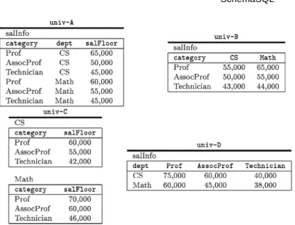
Fig. 2. Representing similar information using different schemas in multiple databasesuniv-A, univ-B, univ-C,anduniv-D.
(c) The expressiondb::rel->denotes the set of names of attributes in the scheme of the relationrelin the databasedb.1
(d) db::reldenotes the set of tuples in the relationrelin the databasedb. (e) db::rel.attrdenotes the set of values appearing in the column named
attrin the relationrelin the databasedb.
(2) A variable declaration is of the form<range> <var>where<range>is one of the range specifications above and <var> is an identifier. An identi-fier <var> is said to be a variable if it is declared as a variable by an expression of the form <range> <var> in the from clause. Variables de-clared over the ranges (a) to (e) are calleddb-name,rel-name,attr-name, tuple, anddomain variables, respectively. Any identifier not so declared is a
constant.
As an illustration of the idea of nesting variable declarations, consider the clause from db1-> X, db1::X T. This declares X as a variable ranging over the set of relation names in the databasedb1andTas a variable ranging over the tuples in each relationXin the databasedb1.
The following sections provide several examples demonstrating various ca-pabilities ofSchemaSQL.
The following federation of databases is used as our running example. Con-sider the federation consisting of four databases, univ-A, univ-B, univ-C, and univ-D. Figure 2 shows some sample data in each of these four databases. Each database has (one or more) relation(s) that record(s) the salary floors for employees by their categories and their departments as follows:
1The intuition for the notation is that we can regard the attributes of a relation as written to the
• univ-Ahas a relationsalInfo (category, dept, salFloor).
• univ-Bhas a relationsalInfo (category, dept1, dept2,. . .). Note that the domains of dept1, dept2,. . .are the same as the domain of salFloor in univ-A::salInfo.
• univ-C has one relation for each department with the scheme depti
(category, salFloor).
• univ-D has a relationsalInfo (dept, cat1, cat2,. . .). Note that the do-mains of attributescat1, cat2,. . . are the same as the domain ofsalFloor inuniv-A::salInfo.
Example2.1 [Comparing salaries inuniv-Aanduniv-B]. List the depart-ments inuniv-Athat pay a higher salary floor to their technicians compared with the same department inuniv-B.
(Q1) select A.dept
from univ-A::salInfo A, univ-B::salInfo B, univ-B::salInfo-> AttB
where AttB <> "category" and
A.dept = AttB and
A.category = "technician" and B.category = "technician" and A.salFloor > B.AttB
Explanation. VariablesAandBare (SQL-like) tuple variables ranging over the relationsuniv-A::salInfoanduniv-B::salInfo, respectively. The variable AttB is declared as an attribute name of the relation univ-B::salInfo. It is intended to be adepti attribute (hence, the conditionAttB <> "category" in
thewhereclause). The rest of the query is self-explanatory.
Example2.2 [Comparing salaries inuniv-Canduniv-D]. List the depart-ments inuniv-Cthat pay a higher salary floor to their technicians compared with the same department inuniv-D.
(Q2) select RelC
from univ-C-> RelC, univ-C::RelC C, univ-D::salInfo D
where RelC = D.dept and
C.category = "technician" and C.salFloor > D.technician
Explanation. The variable RelC is declared as a relation name in the databaseuniv-C. Note that in this database there is one relation per depart-ment, and the relation name coincides with department name. Variable C is then declared as a tuple variable on this (variable) relationRelC. The variable D is an (SQL-like) tuple variable ranging over the relation univ-D::salInfo. Note that in univ-D::salInfocategories are represented by attribute names, whose domains consist of the salary floors of the corresponding category. Hence,
D.technicianis the salary floor for categorytechnician(for the tuple repre-sented by tuple variableD).
3. SEMANTICS I: FIXED OUTPUT SCHEMA
In this section, we discussSchemaSQLqueries with a fixed output schema. The topics of dynamic output schema and restructuring views are discussed in the next section.
We first quickly review the semantics of SQL and express it in a manner that makes it possible to realize the semantics ofSchemaSQLby a simple extension.
3.1 SQL Semantics Reviewed
A query in SQL assumes afixedscheme for the underlying database, and maps each database to a relation over a fixed scheme, called theoutputscheme as-sociated with the query. LetDbe the set of all database instances over a fixed scheme. Let a queryQbe of the form2
select attrList, aggList from fromList
where whereConditions group by groupbyList having havingConditions
LetRbe the set of all relations over the output scheme of the query Q. The queryQ induces a function
Q :D→R
from databases to relations over a fixed scheme, defined as follows: LetD∈D be an input database, andTDthe set of all tuples appearing in any relation in
D. Letτ be the set of tuple variables occurring inQ. We define aninstantiation as a functionı : τ→TD which instantiates each tuple variable in Q to some
tuple over its appropriate range. The conditionswhereConditionsin thewhere clause induce a Boolean function, denotedsatw(ı,Q), on the set of all instanti-ations, reflecting whether the conditions are satisfied by an instantiation. This is defined in the obvious manner. LetIQ= {ı |ı is an instantiation for which
satw(ı,Q)=true}denote the set of instantiations satisfying whereConditions. The query assembles each satisfying instantiation into a tuple for the answer relation, via a tuple assembly function, defined below. LetTattrList denote the set of all tuples over the scheme attrListsuch that each value in each tu-ple appears in the databaseD. Then the tuple assembly function is a function tupleQ :IQ→TattrListdefined as follows:
tupleQ(ı)= O “t.A”∈attrList
ı(t)[A].
Here, the predicate “t.A”∈attrListindicates the condition that the attribute denotationt.Aliterally appears in the list of attributesattrListin theselect
2In this article, we restrict attention to single blockSchemaSQLqueries. In keeping with this, we
statement. The symbolN denotes concatenation, andı(t)[A] denotes the re-striction of the tuple ı(t) to the attribute A. For an instantiationı, tupleQ(ı) produces a tuple over the attributesattrListlisted in theselectstatement. SupposeQis a regular query, that is, a query without aggregation. In this case, theaggListis empty and thehavingandgroup byclauses are absent. So, the result ofanSQL query without aggregationis captured by the function
Q(D)=[tupleQ(ı)|ı∈IQ].
Note that SQL has amultisetsemantics. We use [· · ·] instead of{· · ·}to denote multisets.
To account for aggregation, we need the following extension:
Definition3.1 [Equivalence Relation Induced bygroup byClause]. For ı, ∈IQ,ı∼ iff ∀ “t.A”∈groupbyList,ı(t)[A]=(t)[A]. It is easy to see that ∼ is an equivalence relation on IQ. In words, two instantiations (satisfying
the conditions in thewhereclause) are∼-equivalent provided they agree on all attributes appearing in thegroup byclause.
The conditionshavingConditionsin thehaving clauseare a Boolean com-bination of atomic conditions of the formagg(t.att) relOp cand of the form agg1(t.att1) relOp agg2(t.att2). Intuitively, we are only interested in those equivalence classes of ∼ that satisfy havingConditions. For an equivalence classeof∼, letsath(e,Q)=truedenote thatesatisfieshavingConditions. Note that, in practice, checking whether sath(e,Q)=truefor an equivalence class erequires the calculation of any additional aggregations that may appear in the havingclause but not necessarily in theselectclause. We have the following:
Definition3.2 [Valid Equivalence Classes].
EQ= {e|eis an equivalence class of∼andsath(e,Q)=true}.
Let TaggList denote the set of all tuples over the schemeaggList. We define a functionaggregateQ :EQ→TaggListas follows.
aggregateQ(e)=
O “agg(t.B)”∈AggList
agg([(t)[B]|e∈EQ and∈e]).
For a given equivalence classe∈EQ,aggregateQ considers all instantiations in
e, and, for each aggregate operation, sayagg, indicated on the attributet.Bin aggList, it performs the operationaggon themultisetof values associated with this attribute by instantiations ine. Again, we use [· · ·] to denote multisets.
Now, we are ready to describe the tuple assembly associated with aggregate queries. Let Qbe a query involving aggregation. Define a functionaggtupleQ:
EQ→TattrList×TaggListas follows:
aggtupleQ(e)=tupleQ(ı)OaggregateQ(e),
whereıis any instantiation ine. Note that SQL requires the set of attributes in attrList to be a subset of those in groupbyList. Hence, tupleQ(ı) is the same for all instantiationsı∈e, and thusaggtupleQ(e) is well defined, for any
Finally, theresult of an aggregate SQLquery is captured by the function Q(D)=[aggtupleQ(e)|e∈EQ].
3.2 Semantics ofSchemaSQLQueries
The semantics ofSchemaSQLis obtained as a natural extension of that of SQL. ASchemaSQLqueryQis of the form:
select itemList, aggList from fromList
where whereConditions group by groupbyList having havingConditions
whereitemListis a list of db-name, rel-name, attr-name, and domain variables; aggListis a list of expressions of the formagg(X)where aggis an aggregate function, andXis a db-name, rel-name, attr-name, or domain variable;fromList is a list of variable declarations;groupbyList is a list of db-name, rel-name, attr-name, and domain variables; and the conditions in the where and having clauses are analogous to SQL. The main difference with an SQL query is the availability of additional variable types, in addition to the usual SQL tuple variables.
Let Dbe the set of all federation database instances. Let Rbe the set of all relations over the output scheme of the query Q. The query Q induces a function
Q :D→R
from federations to relations, defined as follows. Let D∈Dbe an input feder-ation, andOD the set of all items (database names, relation names, attribute
names, tuples, and values) appearing inD. LetV be the set of variables occur-ring in Q. We define aninstantiationas a functionı : V→OD which
instan-tiates each variable inQ to some item over its appropriate range.Throughout this article, we assume that any instantiation ı is extended in such a way that for a literal constant c, ı(c)=c.In defining the semantics ofSchemaSQLqueries, we find the following definitions useful. Identifiers in typewrite font (e.g.,db) can be constants or variables.
Definition3.3 [Admissibility]. An instantiationıisadmissibleprovided, it satisfies the following conditions:
—whenever -> D is a declaration in the from clause, ı(D) is the name of a database in the federation.
—wheneverdb-> R is a declaration in the from clause,ı(R) is the name of a relation in the databaseı(db).
—wheneverdb::rel-> Ais a declaration in thefromclause,ı(A) is an attribute name in the relationı(rel) in the databaseı(db).
—wheneverdb::rel Tis a declaration in thefromclause,ı(T) is a tuple in the relationı(rel) in the databaseı(db).
—wheneverdb::rel.attr Vis a declaration in thefromclause,ı(V) is a value that appears in the columnı(attr) of the relationı(rel) in the databaseı(db). —whenever T.attr V is a variable declaration in the from clause, ı(V)=
ı(T)[ı(attr)].
Definition 3.3 precisely captures the notion of an appropriate range for a variable.
Definition3.4 [Validity]. Letsat(ı,Q) be a Boolean function on the set of all instantiations, induced by the conditions in thewhereclause. An instantiation ıisvalidprovided (a) it is admissible, and (b)sat(ı,Q) is true.
The conditions in the where clause as well as additional conditions induced by the presence of certain patterns involving tuple variables is captured in Definition 3.4. We now define,
IQ= {ı|ıis a valid instantiation}. (1)
The query assembles each satisfying instantiation into a tuple for the answer relation, as follows. Let TitemList denote the set of all tuples over the scheme itemListsuch that each value in each tuple appears in the federationD. Then the tuple assembly function is a function tupleQ : IQ→TitemList defined as follows:
tupleQ(ı)= O
s∈itemList
ı(s), (2)
wheresis a db-name, rel-name, attr-name, or domain variable. For an instan-tiationı,tupleQ(ı) produces a tuple over the list of objectsitemListlisted in theselectstatement.
3.2.1 Queries with Fixed Output Schema and No Aggregation. SupposeQ is aSchemaSQLquery without aggregation. In this case, the result of the query is captured by the function
Q(D)=[tupleQ(ı)|ı∈IQ]. (3)
Similar to SQL,SchemaSQL’s semantics is based on multisets. Multisets are distinguished from sets with the use of [. .] instead of{. .}.
It is not hard to see that the formal semantics captured by these definitions exactly correspond to the intuitive semantics discussed earlier for Queries Q1 and Q2 of Section 2.
3.3 Aggregation with Fixed Output Schema
In SQL, we are restricted to “vertical” (or column-wise) aggregation on a pre-determinedset of columns, whileSchemaSQLallows “horizontal” (or row-wise) aggregation, and also aggregation over more general “blocks” of information. Before we illustrate these points with examples, we provide a formal develop-ment of the semantics.
3.3.1 Semantics of Aggregation with Fixed Output Schema. Let Q be a SchemaSQLquery involving aggregation. Similar to the development of SQL
semantics, we define the equivalence relation∼on the instantiationsIQ, and
the set EQ of equivalence classes of ∼ that satisfy thehavingConditions for
SchemaSQLqueries.
Definition3.5 [Equivalence Relation Induced bygroup byClause]. For ı, ∈IQ, ı∼ iff ∀“v”∈groupbyList, ı(v)=(v). It is straightforward to see
that ∼ is an equivalence relation on IQ. Intuitively, two instantiations are ∼-equivalent provided they agree on all variables appearing in the group by clause. We denote byEQ the set of equivalence classes ofIQ under∼.
Definition3.6 [Valid equivalence classes].
EQ= {e|eis an equivalence class of∼andsath(e,Q)=true}, (4) where sath(e,Q)=true means equivalence classs satisfies the havingCondi-tions.
LetTaggList denote the set of tuples over the scheme aggList. We define a functionaggregateQ :EQ→TaggListas follows:
aggregateQ(e)= O “agg(v)”∈aggList
agg([(v)|e∈EQ and∈e]). (5)
For a given equivalence classe∈EQ, aggregateQ considers all instantiations
ine, and, for each aggregate operation, sayagg, indicated on the variablevin aggList, it performs the operationaggon themultisetof values associated with this variable by instantiations ine.
LetQbe a query involving aggregation. We define the tuple assembly func-tionaggtupleQ:EQ→TitemList×TaggListas follows:
aggtupleQ(e)=tupleQ(ı)OaggregateQ(e), (6) whereıis any instantiation ine. InSchemaSQL, we require the set of variables in itemList to be a subset of those in groupbyList. Hence, tupleQ(ı) is the same for all instantiationsı∈e, and thusaggtupleQ(e) is well defined, for any equivalence classeinEQ.
Finally, the result of aSchemaSQLquery with aggregation is captured by the function
Q(D)=[aggtupleQ(e)|e∈EQ]. (7)
We now provide some examples illustrating aggregation inSchemaSQL. Example 3.1 [Horizontal Aggregation and Aggregation through Multiple Relations]. The query
(Q3) select T.category, avg(T.D) from univ-B::salInfo-> D,
univ-B::salInfo T where D <> "category" group by T.category
computes the average salary floor of each category of employees overall de-partments inuniv-B. This captures horizontal aggregation. The conditionD<>
“category”enforces the variableDto range over department names. Hence, a knowledge of department names (and even the number of departments) is not required to express this query. Alternatively, we could enumerate the depart-ments, that is, using the condition(D=“Math” or D=“CS” or. . .).3By contrast, the query
(Q4) select T.category, avg(T.salFloor) from univ-C-> D,
univ-C::D T group by T.category
computes a similar information from univ-C. Notice that the aggregation is computed over a multiset of values obtained fromseveral relationsinuniv-C. In a similar way, aggregations over values collected from more than one database can also be expressed. Block aggregations of a more sophisticated form are illustrated in Example 4.3.
4. SEMANTICS II: DYNAMIC OUTPUT SCHEMA AND RESTRUCTURING VIEWS
The result of an SQL query (or view definition) is a single relation. Our discus-sion in the previous section was limited to the fragment ofSchemaSQLqueries that produce one relation, with a fixed schema, as output. In this section, we provide examples to demonstrate the following capabilities ofSchemaSQL: (i) declaration of dynamic output schema, (ii)restructuring views, and (iii) inter-action between dynamic output schema creation and aggregation.
We illustrate the capabilities of SchemaSQLfor the generation of an out-put schema which can dynamically depend on the contents of the inout-put in-stance (i.e., the databases in the federation). While aggregation in SQL is re-stricted to vertical aggregation on a predetermined set of columns, we have so far seen that SchemaSQLcan express horizontal aggregation and aggre-gation over more general “blocks” (see Example 3.1, Q3 and Q4). In this sec-tion, we shall see that the combination of dynamic output schema and meta-data variables, namely, db-name, rel-name, and attr-name variables, allows us to express more powerful aggregations such as vertical aggregation on a variable number of columns and aggregation on a variable number of blocks as well.
4.1 Restructuring Without Aggregation
We first illustrate the ideas and expressive power ofSchemaSQLfor performing restructuring, using examples. Formal development will follow.
Example 4.1 [Restructuring univ-B Database into the Schema of univ-A Database]. Consider the relation salInfo in the database univ-B. The
3An elegant solution would be to specify some kind of “type hierarchy” for the attributes, which
can then be used for saying “Dis an attribute of the followingkind”, rather than “Dis one of the following attributes”. Our proposed extension toSchemaSQL, discussed in Section 6.2, addresses this issue.
following SchemaSQLview definition restructures this information into the format of the schema ofuniv-A::salInfo.
(Q5) create view BtoA::salInfo(category, dept, salFloor) as select T.category, D, T.D
from univ-B::salInfo-> D, univ-B::salInfo T where D <> ‘category’
Explanation. Two variables are declared in thefromclause:Tis a tuple vari-able ranging over the tuples of relationuniv-B::salInfo, andDis an attribute-name variable ranging over the attributes ofuniv-B::salInfo. The condition in thewhereclause forcesDto be a department name. Finally, each output tuple (T.category,D,T.D)lists the category, department name, and the correspond-ing salary floor (which is in the format ofuniv-A::salInfo).
Note that corresponding to each tuple in theuniv-B::salInfoformat,Q(5) generates several tuples in theuniv-A::salInfoscheme. The mapping, in this respect, is one-to-many. But eachinstantiation of the variables in the query, actually contributes to one output tuple.
The following example illustrates restructuring involving dynamic creation of output schema.
Example 4.2 [Restructuring univ-A database into the schema of univ-B database]. This view definition restructures data inuniv-A::salInfointo the format of the schemauniv-B::salInfo.
(Q6) create view AtoB::salInfo(category, D) as select A.category, A.salFloor
from univ-A::salInfo A, A.dept D
Explanation. Each tuple ofuniv-A::salInfocontains the salary floor for one category in a single department, while each tuple ofuniv-B::salInfo con-tains the salary floors for one category in every department. Intuitively, all tuples inuniv-A::salInfocorresponding to the same category are grouped to-gether and “merged” to produce one output tuple.
Another aspect of this restructuring view is the use of variables in thecreate viewclause. The variableDincreate view AtoB::salInfo(category, D)is de-clared as a domain variable ranging over the values of thedeptattribute in the relationuniv-A::salInfo. Hence, the schema of the viewAtoB::salInfois “dy-namically” declared as AtoB::salInfo(category, dept1,. . ., deptn), where dept1,. . ., deptnare the values occurring in thedeptcolumn in the relation univ-A::salInfo.
The restructuring in this example corresponds to a many-to-one mapping from instantiations to output tuples.
As demonstrated by the previous examples, the semantics of restructuring in the context of a dynamically declared output schema has two aspects to it: (i) the determination of the output schema itself, and (ii) the formatting of
data to conform to the schema determined in (i). In this section, we formalize these concepts. We illustrate our development of the semantics by revisiting Example 4.2.
Let aSchemaSQLqueryQbe a view definition of the form create view db::rel(attr1,..., attrn) as select obj1,..., objn
from fromList
where whereConditions
where db, relare constants or db-name, rel-name, att-name, or domain vari-ables;attr1,. . .,attrnare all constants or one of them is a db-name, rel-name, att-name, or domain variable and the rest are constants; andobj1,. . .,objnare db-name, rel-name, att-name, or domain variables.
We first define some useful notions. Recall thatIQ is the set of valid
instan-tiations (of the variables declared in thefromclause) that satisfy the conditions in thewhereclause, as defined in Section 3.2.
Definition4.1 [Instantiations contributing to the same output relation]. For two instantiationsı,∈IQ, we defineı≡, providedı(db)=(db) andı(rel)=
(rel). Clearly≡is an equivalence relation.
Determination of Output Schema. Each instantiationı∈IQproduces a view
of a database namely,ı(db), containing a relation namedı(rel), whose scheme consists of the attribute setattrsetQ(ı)= {(attr)|attr∈ {attr1,. . .,attrn}, ∈ IQ, ≡ı}. Thus, each≡-equivalence class of instantiations defines one relation
scheme in the output view. For example, in Example 4.2, all instantiationsı∈
IQ are≡-equivalent, and this one equivalence class produces a view containing
a database calledAtoB, containing one relation namedsalInfo, with the scheme
{category,CS,Math,. . .}.
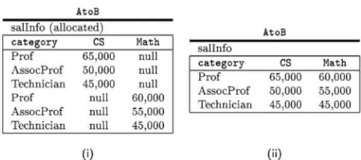
Formatting Data to Fit the Schema. There are two aspects to this. First, the output computed by the SchemaSQL query defining the view has to be properlyallocatedto conform to the output schema declared in thecreate view statement. This by itself might in general result in null values, which we can eliminate by identifying maximal subsets of “related” tuples and “merging” them. These ideas are made precise below.
As seen above, an instantiation ı∈IQ contributes to a view of a database
ı(db) containing a relation namedı(rel) with a scheme given by attrsetQ(ı).
The instantiations≡-equivalent toıcontribute to a relation,allocateQ(ı), over
the attribute setattrsetQ(ı), as follows. For each instantiation∈IQ such that
≡ı, allocateQ(ı) contains a tuple t, defined as follows. Let A∈attrsetQ(ı).
Then
t[A]=
½
(objk), whenever A=(attrk) nul l, otherwise.
Figure 3(i) showsallocateQ6(ı) for the view (Q6) defined in Example 4.2, where ıis any instantiation (recall all of them are≡-equivalent).
Secondly, merging of tuples inallocateQ(ı) is formalized as follows: LetDOM denote the union of all domains of all attributes of all relations involved in the
Fig. 3. (i) The relationallocateQ6(ı) and (ii) the final result after merging.
federation, together with the null value,null. Define a partial order onDOM, by settingnull ≤ v,∀v ∈DOM. In particular, note that any two distinct non-null values are incomparable. Theleast upper bound,lub, of two values inDOMis defined in the obvious way.
lub(u,v)= u, ifv≤u v, ifu≤v undefined, otherwise. We now have the following:
Definition4.2 [Merging a Pair of Tuples]. Two tuplest1,t2over a relation scheme R= {A1,. . .,An} are mergeable provided for each i=1,. . .,n, either t1[Ai]=t2[Ai], or at least one of t1[Ai] or t2[Ai] is a null. Suppose t1 and t2
are mergeable. Then their merge, denoted t=t1Jt2, is defined as t[Ai]=
lub(t1[Ai],t2[Ai]),i=1,. . .,n.
Clearly, the operatorJis commutative and associative, and it can be easily extended to any set ofmergeabletuples. It will be convenient below to extend the operator Jto any relation containing an arbitrary (i.e., not necessarily mergeable) set of tuples. The idea is to partition the relation into sets of merge-able tuples, and merge the tuples in each partition. Notice that mergeability is not a transitive relation: for example, tuplet1=(a,⊥) is mergeable with each of the tuplest2=(a,b) andt3=(a,b0), which themselves are not mergeable. Thus, in partitioning a relation into sets of mergeable tuples, choice arises in grouping tuples. From the point of view of the meaning of the tuples, the choices may be made arbitrarily. So, for instance, we may merget1andt2above (and leavet3 alone) or merget1andt3. While the results look physically different, the mean-ing is the same. Intuitively, we need any “maximal” partition of a relation that respects mergeability, formalized below.
Definition4.3 [Maximal Partitions]. A partition P= {r1,. . .,rk} of a rela-tionrisvalidprovided for each blockri, the tuples inriare pairwise mergeable,
1≤i ≤k. Define a partial order≤on partitions as follows:4 P
1 ≤P2 provided
∀ri ∈P1:∃sj ∈P2:ri ⊆sj. A partitionP is amaximalvalid partition provided
for every valid partitionP0:P ≤P0⇒P0=P.
The following easily established result reveals the significance of maximal valid partitions.
LEMMA4.1 [MAXIMALPARTITIONS]. Let r be a relation andPbe any maximal valid partition of r. Then the following holds:(i)for each block ri ∈P,the tuples
in ri are pairwise mergeable;(ii)for any two distinct blocks ri,rj ∈P,the tuples
ri∪rj are not pairwise mergeable,that is,there is a pair of tuples t,t0∈ri∪rj
such that they are not mergeable.
We suppress the obvious proof. Finally, we can define the result of applying a merge operator to a relation as follows:
Definition4.4 [Merging a Relation]. Letrbe a relation andP = {r1,. . .,rk} be any maximal valid partition ofr. Then,Jr= {J(ri)|ri ∈P}.
Finally, we can define the semantics of view definitions inSchemaSQL with-out aggregation as follows:
Definition4.5 [Semantics of Restructuring Views without Aggregation]. Let Q be theSchemaSQLquery that defines a view V. Then the materialization of V consists of one relation for each≡-equivalence class of instantiations in
IQ. For an equivalence class [ı], for anyı ∈ IQ, the corresponding relation is
determined byJallocateQ(ı).
As an example, the final output produced by the view definition (Q6) in Example 4.2 is a view of a database A2B containing a relation salInfo(category, CS, Math)as shown in Figure 3(ii).
4.2 Aggregation with Dynamic View Definition
In Section 3, we illustrated the capability of SchemaSQL for computing (i) horizontal aggregation and (ii) aggregation over blocks of information collected from one or more relations, or even databases. In this section, we shall see that when SchemaSQLaggregation is combined with its view definition facility, it is possible to express vertical aggregation over a variablenumber of columns or blocks of data, determined dynamically by the input instance. The following examples illustrate this point.
Example4.3 [Block Aggregation: Fixed and Dynamic Output Schemas]. Suppose in the database univ-D in Figure 2, there is an additional relation faculty(dname, fname)relating each department to its faculty, such as, (math, arts and sciences), (physics, arts and sciences), (cs, engineering and comp sci), etc.
The first query uses a fixed output schema. The second query is identical to the first except for acreate viewexpression that defines a dynamic output schema:
(Q7) select U.fname, avg(T.C) from univ-D::salInfo-> C,
univ-D::salInfo T, univ-D::faculty U
where C <> "dept" and T.dept = U.dname group by U.fname
Q7 computes, for each faculty, the faculty-wide average floor salary ofall em-ployees (over all departments) in the faculty. Notice that the aggregation is performed over ‘rectangular blocks’ of information.
Consider now the following view definition Q8, which is essentially defined using the query Q7.
(Q8) create view averages::salInfo(faculty, C) as select U.fname, avg(T.C)
from univ-D::salInfo-> C, univ-D::salInfo T, univ-D::faculty U where C <> "dept" and
T.dept = U.dname group by U.fname
The view defined by Q8 actually computes, for each faculty, the average floor salary ineach categoryof employees (over all departments) in the faculty. This is achieved by using the variableC, ranging over categories, in the dynamic output schema declaration through the create view statement. The schema of the output has the form {faculty, Prof, AssocProf, Technician,. . .}, namely, the variable C in the view definition represents its value in the set of valid instantiations, and hence the output schema depends on the input data.
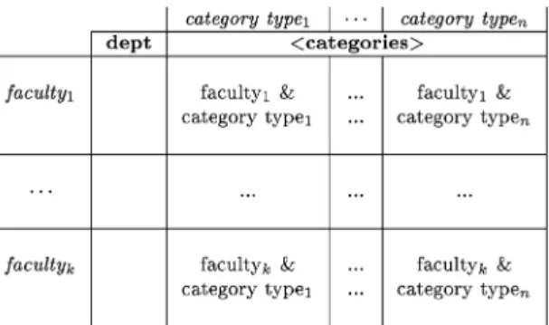
Example4.4 [Aggregation on a Variable Number of Blocks]. Let us add yet another relation to the database univ-D of Figure 2. The relation empType(category, type) lists the categories, and their types, for example, (prof, teaching faculty), (assoc prof, teaching faculty), (technician, technical staff), (secretary, administrative staff), etc. Consider the query:
(Q9) create view averages::salInfo(faculty, Y) as select U.fname, avg(T.C)
from univ-D::salInfo-> C, univ-D::salInfo T, univ-D::faculty U, univ-D::empType E, E.type Y
where C <> "dept" and T.dept = U.dname and E.category = C group by U.fname
Figure 4 depicts relationuniv-D::salInfo, and the “blocks” upon which the aggregation is carried out. Each block corresponds to a faculty and an employee type.
Fig. 4. univ-D::salInforelation. The schema components appear in bold face font. The “facultyi
& category typej” rectangles are the blocks upon which the aggregation is carried out.
The schema of the output relation is
averages::salInfo(faculty,teachingfaculty,technicalstaff,. . .) and each tuple in the output lists a faculty, such as “arts and sciences”, and the corresponding average salary floors for the employees in each of the category types “teaching faculty”, “technical staff ”, “administrative staff ”, etc.
4.2.1 Semantics of Aggregation with Dynamic View Definition. The seman-tics of restructuring (via view definition) with aggregation involves putting to-gether the ideas behind each of these operations. Intuitively, as explained in Section 4.1, the instantiations≡-equivalent toı∈IQ produce (in the view) one
relation in a database whose scheme consists of the attributesattrsetQ(ı), as
defined in that section. The tuples for this relation are obtained by computing the aggregations listed in theaggListin theselectstatement with respect to each valid equivalence class of instantiations that agree on the variables listed in thegroup byclauseas well ason the variables appearing in thecreate view statement, and then performing the necessary merging. The reason for includ-ing the variables in the create view statement is that they specify an implicit group by. This intuition is formalized below. Consider the SchemaSQL view definition Q, below:
create view db::rel(attr1,..., attrn) as select itemList, aggList
from fromList
where whereConditions group by groupbyList having havingConditions
Definition 4.6 [Equivalence Relation Induced by Group by and Create View Clauses]. For two instantiationsı, ∈ IQ, we define ı#, provided for each
o ∈ groupbyList,ı(o)=(o), and for each variableX occurring in thecreate viewstatement,ı(X)=(X). Clearly, # is an equivalence relation.
Similar to previous cases, we denote byEQ the set of equivalence classes of IQ under # that satisfy thehavingConditions:
Definition4.7 [Valid Equivalence Classes].
EQ = {e|eis an equivalence class of # andsath(e,Q)=true}.
The notions ofaggregateQ(e),aggtupleQ(e), andsath(e,Q) for an equivalence classe∈ EQ, are defined analogously to the way they were defined in Section
3.3. The only difference is that the equivalence relation # is used instead of∼. aggregateQ(e) = O
“agg(o)”∈aggList
agg([(o)|e∈EQ and∈e])
aggtupleQ(e) = tupleQ(ı)OaggregateQ(e) whereıis any instantiation in the equivalence classe.
The concept of allocatingtuples computed above according to the various output schemas dynamically created by the instantiations can be formalized in a way similar to what was done in Section 4.1, and we suppress these obvious details for brevity. Recall that the schema of each output relation is determined by one equivalence class ofIQ under the≡relationship. Let aggallocateQ (ı)
denote the allocated relation determined by the≡-equivalence class ofı∈IQ.
The concept of merging, defined in Definitions 4.2 and 4.4, can now be directly applied to compute the final output. Thus, for each instantiationı∈IQ, the ≡-equivalence class ofıcontributes to the relationJaggallocateQ (ı), over the
schemaı(db) ::ı(rel)(attrsetQ(ı)).
As an example, it is easy to verify that the view defined by Q8 indeed com-putes for each faculty, the category-wise floor salary averages. Before closing this section, we note that the combination of dynamic output schema declara-tion withSchemaSQL’s aggregation mechanism makes it possible to express many other novel forms of aggregation as well. Further, note that the exam-ples in this and previous sections were in the context of a single database, demonstrating some of the applications ofSchemaSQLfor a single database environment.
5. IMPLEMENTATION
In this section, we describe the architecture of a system for implementing a mul-tidatabase querying and restructuring facility based onSchemaSQL. A high-light of our architecture is that it builds on existing architecture of SQL in a nonintrusive way, requiring minimal extensions to prevailing database tech-nology. This makes it possible to build aSchemaSQLsystem on top of (already available) SQL systems. We also identify novel query optimization opportuni-ties that arise in a multidatabase setting.
The architecture consists of aSchemaSQLserver that communicates with the local databases in the federation. We assume that the meta-information comprising component database names, names of the relations in each database, names of the attributes in each relation, and possibly other useful information (such as statistical information on the component databases, use-ful for query optimization) are stored in theSchemaSQLserver in the form of a relation calledFederation System Table(FST).
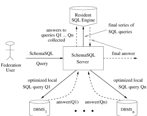
Fig. 5. SchemaSQL — implementation architecture.
Figure 5 depicts our architecture for implementingSchemaSQL. At a high level, global SchemaSQL queries are submitted to the SchemaSQL server, which determines a series of local SQL queries and submits them to the lo-cal databases. The SchemaSQL server then collects the answers from local databases, and, using its own residentSQL engine, executes a final series of SQL queries against the answers collected above, to produce the answer to the global query. Intuitively, the task of the SchemaSQL server is to com-pile the instantiations for the variables declared in the query, and enforce the conditions, groupings, aggregations, and mergings to produce the out-put. Many query optimization opportunities at different stages, and at differ-ent levels of abstraction, are possible, and should be employed for efficiency (see discussions in Section 6.1). Algorithms 5.1 and 5.2 give detailed accounts of our query processing strategy for the fixed and dynamic output schema, respectively.
Query processing in aSchemaSQLenvironment consists of two major phases. In the first phase, tables called VIT’s (Variable Instantiation Tables) corre-sponding to the variable declarations in thefromclause of aSchemaSQLquery are generated. The schema of a VIT consists of all the variables in one or more variable declarations in the fromclause, while its contents correspond to in-stantiations of these variables.VIT’s are materialized by executing appropriate SQL queries on the FST and/or component databases.In the second phase, the SchemaSQLquery is rewritten into a series of one or more SQL queries against the VITs with the property that the result of the series of queries against the
VITs is identical to that of the originalSchemaSQLquery against the feder-ation. The result so obtained is appropriately restructured for presentation to the user.
For ease of exposition, we first consider (Section 5.1)SchemaSQLqueries with a fixed output schema and then present the algorithm for handling queries with a dynamic output schema (Section 5.2).
5.1 ProcessingSchemaSQLQueries with a Fixed Output Schema
We assume that the FST has the schemeFST(db-name, rel-name, attr-name). Also, we refer to the db-name, rel-name, and attr-name variables (defined in Definition 2.1) collectively asmeta-variables.
Our algorithm below considers SchemaSQL queries with a fixed output schema, possibly with aggregation. The algorithm consists of two phases as explained above. In order to facilitate the reader to follow the development, we break the presentation of the algorithm after each phase and follow it with an illustrative example.
ALGORITHM 5.1. SchemaSQL Query Processing—Fixed Output Schema Input: ASchemaSQLquery with aggregation and with a fixed output schema.
Output: The result of the query.
Method:
Phase I:Corresponding to a set of variable declarations in thefromclause, createV I Ts using one or more SQL queries against some local databases and/or the FST.
Phase II:Rewrite the originalSchemaSQLquery against the federation into an “equivalent” query against the set ofV I Trelations and compute it using the resident SQL server.
Phase I
(0)Rewrite the inputSchemaSQLstatement into the following form such that the conditions in thewhereandhavingclauses are in conjunctive normal form.
select itemList, aggList
from hrang e1iV1, . . ., hrang ekiVk
where hcond1iand. . .andhcondmi
group by groupbyList having havingConditions
We assume an ordering on the variable declarations in thefromclause: If a variableVj
appears in the range of another variableVi, that is, inhrangeii, then we sayVidepends
on Vj, denotedVj ≺Vi. We will assume that wheneverVj ≺Vi, the declaration ofVj
comes before that ofVi in thefrom clause. It is trivial to reorder the declarations in a
givenSchemaSQLquery to meet this condition.
(1) Consider each variable declarationhrangeiiVi, 1≤i≤k. The following cases arise:
(a)Viis a meta-variable: In this case, all variables in the declarationhrangeiiVimust
be meta-variables. As an optimization issue, notice that it is sufficient to create VITs for just those meta variables that are maximal (among meta-variables) with respect to the ordering≺: As we will discuss below, the VIT for a maximal meta-variableVialso
contains the instantiations for all meta-variablesVj such thatVj ≺ Vi. Create a VIT
forVi,VITVi as follows: the schema ofVITVi consists ofViand all variablesVjsuch that
Vj≺Vi; the contents ofVITViare obtained using an appropriate SQL query against the
FST. For example, assume thefromclause contains the declarations-> DandD::r-> Adeclaring db-name and attr-name variablesDandA, whereris a constant (relation
name). The VIT forDwill have the schema{D, A}. Its contents can be obtained using the SQL query
select db-name as D, attr-name as A
from FST
where rel-name = r
Notice thatVITDincludes instantiations for the attr-name variableA, and thus we can
save on creating a separate VIT for A. We can further optimize the query processing by enforcing conditions of the formU relOpc(orcrelOpU) in thewhereclause of the originalSchemaSQLquery, if any, at this time, providedU is a variable in the schema ofVITVi,relOpis a comparison operator, andcis a constant.
(b)Vi is a tuple variable: Let the declaration forTbedb::rel T, wheredb(rel) can be
constant or variable. Determine the schema ofVITT as follows.
(i) Include all meta-variables appearing indb::rel, if any, in the schema ofVITT.
(ii) IfT.a, whereais a constant, appears in the query (in theselect,where,5 group by, orhavingclauses), includeTain the schema ofVITT. Here, the identifierTais
obtained by concatenating the tuple variableTwith the attribute namea.
(iii) For each domain variable declarationT.a V, whereais a constant, includeVin the schema ofVITT.
For each domain variable declaration T.A V, where A is an attr-name variable, include bothAandVin the schema ofVITT.
(iv) If, for an attr-name variableA,T.Aappears in theselect,where,group by, orhaving
clauses, then include bothAandTAin the schema ofVITT.
Next, obtain the contents ofVITTby submitting SQL queries to component databases,
and computing their union, as follows.
(i) Identify the meta-variables in the schema of VITT. These include any variables
indb::rel, and possibly some attr-name variables. Obtain the bindings for these variables by executing an SQL query on their VITs.
(ii) For each binding obtained, generate one SQL query and submit it to the appropriate component database, in order to retrieve the relevant tuples from that database that pertain to the binding on the meta-variables. Push each condition of the formT.att relOp c(c relOp T.att),T.A relOp c(c relOp T.A), andV relOp c(c relOp V), whereattandcare constants,Ais an attr-name variable, andVis a domain variable declared using T, in thewhereclause of the originalSchemaSQLquery into thewhere
clause of the SQL query to be submitted, above.
(iii) Finally, obtain the contents ofVITTas the union of the SQL queries submitted to
component databases. If only one component database is involved,i.e.ifdbin the declarationdb::rel Tis a constant, then the union can be expressedwithinone SQL query submitted to the component databasedb.
This completes Phase I of the algorithm.
Notice that no separate VITs are needed for domain variables, as their instanti-ations are captured by the VITs for their associated tuple variables. Exampe 5.1 illustrates generation of VITs for meta and tuple variables.
Example5.1 [Illustrating Phase I:Generating VITs]. In this example, we illustrate the Phase I of the algorithm using a variant of query Q2 of Example 2.2:
5IfT.aappearsonlyin thewhereclause, in the formT.a relOp cwherec is a constant, then
(Q2’) select RelC, C.salFloor from univ-C-> RelC,
univ-C::RelC C, univ-D::salInfo D
where RelC = D.dept and
C.salFloor > D.technician and C.category = "technician"
The query contains declarations for one meta variableRelC, which is a rel-name variable, and two tuple variablesCandD. Here is how Phase I of the algorithm will proceed to construct the VITs for this query. (Notice that as far as Phase I is concerned, aggregation is completely orthogonal.)
The schema of VITRelC is {RelC}(one column). Its contents are generated using the following query to the FST:
select rel-name as RelC from FST
where db-name = "univ-C"
The schema of VITC is {RelC,CsalFloor}. Note that Ccategory need not be included: Thewhere clause condition C.category = "technician" will be enforced within the SQL query to the component database univ-C. VITC is generated as the union of SQL queries to database univ-C as follows: First, bindings for the meta-variableRelC are obtained from its VIT via the trivial query:
select RelC from VITRelC
Let{r1,. . .,rn}be the answer to the above query.VITCis obtained by submitting
the following SQL query to the databaseuniv-C.
select ’r1’ as RelC, salFloor as CsalFloor from r1
where category = "technician" UNION
...
UNION
select ’rn’ as RelC, salFloor as CsalFloor
from rn
where category = "technician"
Finally, the schema ofVITD is{Ddept,Dtechnician}, and its contents are ob-tained via the following SQL query to the databaseuniv-D:
select dept as Ddept, technician as Dtechnician from salInfo
Algorithm 5.1SchemaSQLQuery Processing(cont’d.) Phase II
(1)Execution of this phase happens in theSchemaSQLserver. TheSchemaSQLquery is rewritten into an equivalent conventional SQL query on the VIT’s generated in Phase I, as follows: To simplify the presentation, we use the concept of the Joined Variable Instantiation Table(JVIT). As the name suggests, JVIT is the (natural) join of the VITs generated for the various meta-variables and tuple variables during Phase I. In the creation of the JVIT, we enforce the remaining conditions, if any, in thewhere clause of the originalSchemaSQLquery. However, these conditions need to be syntactically rewritten so they make sense against the schema of the JVIT.
Recall that allwhereclause conditions involving a comparison with a constant were already enforced in Phase I. The remaining conditions must have the formobj1 relOp obj2, whereobj1andobj2are either variables, or qualified attributes of the formT.aor
T.A. We need to rewrite these conditions by renaming the obj’s (variables and/or qualified attributes) as follows:
(i) Replace each occurrence of variableVbyVITU.V, whereVITUis the VIT corresponding
toV. It is possible thatUis different fromV, since VITs are generated only for certain variables and the instantiations for the remaining variables are obtained from these (see Phase I).
(ii) Replace each occurrence of a qualified attributeT.a(orT.A) byVITT.Ta(orVITT.TA). (2)AssumeVITV1,. . .,V I TVn are all the variable instantiation tables generated in
Phase I. Let{U1,. . .,Um}be the union of their schemas. Properly qualify eachUiwith
the VIT whose schema contains Vi. For example, ifUi isTa, then its qualified version
is VITT.Ta. IfUi appears in the schemas of several VITs, break the tie arbitrarily for
the purpose of qualification. Let{V I TU1.U1,. . .,V I TUm.Um}represent the qualified set.
Then obtain the joined variable instantiation table using the following SQL query:
create view JVIT(U1,. . .,Um) as
select VITU1.U1,. . .,VITUm.Um
from VITV1,. . .,VITVn
where (rewritten where clause) and
(natural join conditions)
Here, “rewritten where clause” is obtained by rewriting the remainingwhereclause conditions as pointed out above, and “natural join conditions” consist of conditions of the formVITVi.attr=VITVj.attrfor all pairs of VITsVITViandVITVjand all attributes
attrthat are common to the schemas of these VITs.
(3)Finally, generate a SQL query from the originalSchemaSQLquery to produce the final output, as follows.
select itemList’, aggList’
from JVIT
group by groupbyList’
having havingConditions’
where, itemList’(respectively, aggList’, groupbyList’, havingConditions’) is ob-tained fromitemList(respectively,aggList, groupbyList, havingConditions) in the originalSchemaSQLquery by replacing every occurrence ofT.abyTaand ofT.AbyTA. Note that the generation of JVIT and the final SQL query can be combined in one step. We chose to divide it into two steps for clarity of exposition. Further, it also simplifies our presentation of the query processing algorithm forSchemaSQLqueries with dynamic output schemas in Section 5.2. In fact, since we generated JVIT as a view, a natural option for the the resident SQL engine’s query optimizer is to use query rewriting (rather than materializing JVIT) to process the final query in one step.
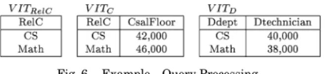
Fig. 6. Example—Query Processing. We now present an example that illustrates our algorithm.
Example5.2 [Illustrating Phase II: Computing the Rest]. We continue with the processing of query(Q2’) of Example 5.1. There, we demonstrated how the VITsVITRelC,VITCandVITDare generated. Figure 6 shows these VITs for the federation of Figure 2.
The following SQL query produces the JVIT.
create view JVIT(RelC, CsalFloor, Ddept, Dtechnician) as select VITRelC.RelC, VITC.CsalFloor, VITD.Ddept,
VITD.Dtechnician from VITRelC, VITC, VITD
where VITRelC.RelC = VITD.Ddept and
VITC.CsalFloor > VITD.Dtechnician and VITRelC.RelC = VITC.RelC
In this query, the first two conditions in thewhereclause came from the (rewrit-ten versions of) the first two conditions in thewhere clause of (Q2’). The last condition in the SQL query enforces natural join. Here is the final SQL query.
select RelC, CsalFloor
from JVIT
Notice thatC.salFlooris replaced byCsalFloor.
Next, let us consider the effect of aggregation. As with Phase I, aggregation remains orthogonal to the processing being done in Phase II. As an illustration, consider the following query from Example 3.1.
(Q3): “find the average salary floor across all departments for each employee category in databaseuniv-B.” This query involves a horizontal aggregation.
select T.category, avg(T.D) from univ-B::salInfo -> D,
univ-B::salInfo T, where D <> "category" group by T.category
Computation of the JVIT for this query is analogous to that for (Q2’): aggrega-tion does not influence this step. Then, the final SQL query would be:
select Tcategory, avg(TD)
from JVIT
group by Tcategory
The following lemma forms the basis for the correctness of our query processing strategy for both fixed and dynamic output schema.