DOI 10.1007/s11263-016-0981-7
Visual Genome: Connecting Language and Vision Using
Crowdsourced Dense Image Annotations
Ranjay Krishna1 · Yuke Zhu1 · Oliver Groth2 · Justin Johnson1 · Kenji Hata1 · Joshua Kravitz1 · Stephanie Chen1 · Yannis Kalantidis3 · Li-Jia Li4 ·
David A. Shamma5 · Michael S. Bernstein1 · Li Fei-Fei1
Received: 23 February 2016 / Accepted: 12 September 2016
© The Author(s) 2017. This article is published with open access at Springerlink.com Abstract Despite progress in perceptual tasks such as image
classification, computers still perform poorly on cognitive tasks such as image description and question answering. Cog-nition is core to tasks that involve not just recognizing, but reasoning about our visual world. However, models used to tackle the rich content in images for cognitive tasks are still being trained using the same datasets designed for per-ceptual tasks. To achieve success at cognitive tasks, models need to understand the interactions and relationships between objects in an image. When asked “What vehicle is the per-son riding?”, computers will need to identify the objects in
an image as well as the relationshipsriding(man, carriage)
andpulling(horse, carriage) to answer correctly that “the person is riding a horse-drawn carriage.” In this paper, we present the Visual Genome dataset to enable the modeling of such relationships. We collect dense annotations of objects, attributes, and relationships within each image to learn these models. Specifically, our dataset contains over 108K images where each image has an average of 35 objects, 26 attributes, and 21 pairwise relationships between objects. We canoni-calize the objects, attributes, relationships, and noun phrases in region descriptions and questions answer pairs to Word-Net synsets. Together, these annotations represent the densest
Communicated by Margaret Mitchell, John Platt, and Kate Saenko.
B
Ranjay Krishna[email protected] 1 Stanford University, Stanford, CA, USA
2 Dresden University of Technology, Dresden, Germany 3 Yahoo Inc., San Francisco, CA, USA
4 Snapchat Inc., Los Angeles, CA, USA
5 Centrum Wiskunde & Informatica (CWI), Amsterdam, The Netherlands
and largest dataset of image descriptions, objects, attributes, relationships, and question answer pairs.
Keywords Computer vision·Dataset·Image·Scene graph·
Question answering·Objects·Attributes·Relationships·
Knowledge·Language·Crowdsourcing
1 Introduction
A holy grail of computer vision is the complete under-standing of visual scenes: a model that is able to name and detect objects, describe their attributes, and recognize their relationships. Understanding scenes would enable impor-tant applications such as image search, question answering, and robotic interactions. Much progress has been made in recent years towards this goal, including image
classifica-tion (Perronnin et al. 2010;Simonyan and Zisserman 2014;
Krizhevsky et al. 2012;Szegedy et al. 2015) and object
det-ection (Girshick et al. 2014;Sermanet et al. 2013;Girshick
2015; Ren et al. 2015b). An important contributing factor is the availability of a large amount of data that drives the statistical models that underpin today’s advances in compu-tational visual understanding. While the progress is exciting, we are still far from reaching the goal of comprehensive scene
understanding. As Fig.1 shows, existing models would be
able to detect discrete objects in a photo but would not be able to explain their interactions or the relationships between
them. Such explanations tend to becognitivein nature,
inte-grating perceptual information into conclusions about the
relationships between objects in a scene (Bruner 1990;
Fire-stone and Scholl 2015). A cognitive understanding of our visual world thus requires that we complement comput-ers’ ability to detect objects with abilities to describe those
Fig. 1 An overview of the data needed to move from perceptual aware-ness to cognitive understanding of images. We present a dataset of images densely annotated with numerous region descriptions, objects, attributes, and relationships. Some examples of region descriptions (e.g.
“girl feeding large elephant” and “a man taking a picture behind girl”) are shown (top). The objects (e.g.elephant), attributes (e.g.large) and relationships (e.g.feeding) are shown (bottom). Our dataset also contains image related question answer pairs (not shown)
objects (Isola et al. 2015) and understand their interactions within a scene (Sadeghi and Farhadi 2011).
There is an increasing effort to put together the next gen-eration of datasets to serve as training and benchmarking datasets for these deeper, cognitive scene understanding and reasoning tasks, the most notable being MS-COCO (Lin et al. 2014) and VQA (Antol et al. 2015). The MS-COCO dataset consists of 300K real-world photos collected from Flickr. For each image, there is pixel-level segmentation of 80 object classes (when present) and 5 independent, user-generated sentences describing the scene. VQA adds to this a set of 614K question answer pairs related to the visual contents of
each image (see more details in Sect.3.1). With this
infor-mation, MS-COCO and VQA provide a fertile training and testing ground for models aimed at tasks for accurate object detection, segmentation, and summary-level image
caption-ing (Kiros et al. 2014;Mao et al. 2014;Karpathy and Fei-Fei
2015) as well as basic QA (Ren et al. 2015a; Malinowski et al. 2015;Gao et al. 2015; Malinowski and Fritz 2014). For example, a state-of-the-art model (Karpathy and Fei-Fei 2015) provides a description of one MS-COCO image in
Fig.1 as “two men are standing next to an elephant.” But
what is missing is the further understanding of where each object is, what each person is doing, what the relationship between the person and elephant is, etc. Without such rela-tionships, these models fail to differentiate this image from other images of people next to elephants.
To understand images thoroughly, we believe three key
elements need to be added to existing datasets: a
ground-ing of visual concepts to language (Kiros et al. 2014),
a more complete set of descriptions and QAs for each
image based on multiple image regions (Johnson et al. 2015),
and aformalized representationof the components of an
image (Hayes 1978). In the spirit of mapping out this com-plete information of the visual world, we introduce the Visual Genome dataset. The first release of the Visual Genome
dataset uses 108,077 images from the intersection of the
YFCC100M (Thomee et al. 2016) and MS-COCO (Lin et al. 2014). Section5provides a more detailed description of the dataset. We highlight below the motivation and contributions of the three key elements that set Visual Genome apart from existing datasets.
The Visual Genome dataset regards relationships and attributes as first-class citizens of the annotation space, in addition to the traditional focus on objects. Recognition of relationships and attributes is an important part of the com-plete understanding of the visual scene, and in many cases, these elements are key to the story of a scene (e.g., the differ-ence between “a dog chasing a man” versus “a man chasing a dog”). The Visual Genome dataset is among the first to pro-vide a detailed labeling of object interactions and attributes, grounding visual concepts to language.1
An image is often a rich scenery that cannot be fully
described in one summarizing sentence. The scene in Fig.1
contains multiple “stories”: “a man taking a photo of ele-phants,” “a woman feeding an elephant,” “a river in the background of lush grounds,” etc. Existing datasets such as Flickr 30K (Young et al. 2014) and MS-COCO (Lin et al. 2014) focus on high-level descriptions of an image.2Instead, for each image in the Visual Genome dataset, we collect more than 50 descriptions for different regions in the image,
pro-viding a much denser and morecomplete set of descriptions
of the scene. In addition, inspired by VQA (Antol et al. 2015), we also collect an average of 17 question answer pairs based on the descriptions for each image. Region-based question answers can be used to jointly develop NLP and vision mod-els that can answer questions from either the description or the image, or both of them.
With a set of dense descriptions of an image and the explicit correspondences between visual pixels (i.e. bound-ing boxes of objects) and textual descriptors (i.e. relation-ships, attributes), the Visual Genome dataset is poised to be the first image dataset that is capable of providing a
struc-turedformalized representationof an image, in the form
that is widely used in knowledge base representations in
NLP (Zhou et al. 2007;GuoDong et al. 2005;Culotta and
Sorensen 2004;Socher et al. 2012). For example, in Fig.1, we
can formally express the relationshipholdingbetween the
womanandfoodasholding(woman,food). Putting together all the objects and relations in a scene, we can represent each image as a scene graph (Johnson et al. 2015). The scene graph representation has been shown to improve semantic image
retrieval (Johnson et al. 2015;Schuster et al. 2015) and image
captioning (Farhadi et al. 2009;Chang et al. 2014;Gupta and
Davis 2008). Furthermore, all objects, attributes and rela-tionships in each image in the Visual Genome dataset are canonicalized to its corresponding WordNet (Miller 1995) ID (called a synset ID). This mapping connects all images in Visual Genome and provides an effective way to consistently
1The Lotus Hill Dataset (Yao et al. 2007) also provides a similar anno-tation of object relationships, see Sec3.1.
2COCO has multiple sentences generated independently by different users, all focusing on providing an overall, one sentence description of the scene.
query the same concept (object, attribute, or relationship) in the dataset. It can also potentially help train models that can learn from contextual information from multiple images
(Figs.2,3).
In this paper, we introduce the Visual Genome dataset with the aim of training and benchmarking the next generation of computer models for comprehensive scene
understand-ing. The paper proceeds as follows: In Sect.2, we provide
a detailed description of each component of the dataset.
Section3provides a literature review of related datasets as
well as related recognition tasks. Section 4 discusses the
crowdsourcing strategies we deployed in the ongoing effort
of collecting this dataset. Section5is a collection of data
anal-ysis statistics, showcasing the key properties of the Visual
Genome dataset. Last but not least, Sect.6provides a set of
experimental results that use Visual Genome as a benchmark. Further visualizations, API, and additional information on
the Visual Genome dataset can be found online.3
2 Visual Genome Data Representation
The Visual Genome dataset consists of seven main
compo-nents:region descriptions,objects,attributes,relationships,
region graphs, scene graphs, and question answer pairs.
Figure4shows examples of each component for one image.
To enable research on comprehensive understanding of images, we begin by collecting descriptions and question answers. These are raw texts without any restrictions on length or vocabulary. Next, we extract objects, attributes and relationships from our descriptions. Together, objects, attributes and relationships comprise our scene graphs that represent a formal representation of an image. In this section,
we break down Fig.4and explain each of the seven
compo-nents. In Sect.4, we will describe in more detail how data
from each component is collected through a crowdsourcing platform.
2.1 Multiple Regions and Their Descriptions
In a real-world image, one simple summary sentence is often insufficient to describe all the contents of and inter-actions in an image. Instead, one natural way to extend this might be a collection of descriptions based on dif-ferent regions of a scene. In Visual Genome, we collect diverse human-generated image region descriptions, with
each region localized by a bounding box. In Fig.5, we show
three examples of region descriptions. Regions are allowed to have a high degree of overlap with each other when the descriptions differ. For example, “yellow fire hydrant” and “woman in shorts is standing behind the man” have very little 3 https://visualgenome.org.
Fig. 2 An example image from the Visual Genome dataset. We show 3 region descriptions and their corresponding region graphs. We also show the connected scene graph collected by combining all of the image’s region graphs. Thetop regiondescription is “a man and a
woman sit on a park bench along a river.” It contains the objects:
man, woman, bench and river. The relationships that connect these objects are:sits_on(man,bench),in_front_of(man,river), and
Fig. 3 An example image from our dataset along with its scene graph representation. The scene graph contains objects (child,
instructor,helmet, etc.) that are localized in the image as bound-ing boxes (not shown). These objects also have attributes:large,
green, behind, etc. Finally, objects are connected to each other through relationships:wears(child,helmet),wears(instructor,jacket), etc
Fig. 4 A representation of the Visual Genome dataset. Each image contains region descriptions that describe a localized portion of the image. We collect two types of question answer pairs (QAs): freeform QAs and region-based QAs. Each region is converted to a region graph
representation of objects, attributes, and pairwise relationships. Finally, each of these region graphs are combined to form a scene graph with all the objects grounded to the image.Best viewed in color
Fig. 5 To describe all the contents of and interactions in an image, the Visual Genome dataset includes multiple human-generated image regions descriptions, with each region localized by a bounding box. Here, we show three regions descriptions on various image regions: “man jumping over a fire hydrant,” “yellowfire hydrant,” and “woman in shorts is standingbehindthe man”
overlap, while “man jumping over fire hydrant” has a very high overlap with the other two regions. Our dataset contains on average a total of 50 region descriptions per image. Each description is a phrase ranging from 1 to 16 words in length describing that region.
2.2 Multiple Objects and Their Bounding Boxes
Each image in our dataset consists of an average of 35
objects, each delineated by a tight bounding box (Fig. 6).
Furthermore, each object is canonicalized to a synset ID
in WordNet (Miller 1995). For example, man would get
mapped toman.n.03 (the generic use of the
word to refer to any human being). Similarly,
person gets mapped to person.n.01 (a human being). Afterwards, these two concepts can be joined to
person.n.01since this is a hypernym ofman.n.03. We did not standardize synsets in our dataset. However, given our canonicalization, this is easily possible leveraging the WordNet ontology to avoid multiple names for one object (e.g. man, person, human), and to connect information across images.
2.3 A Set of Attributes
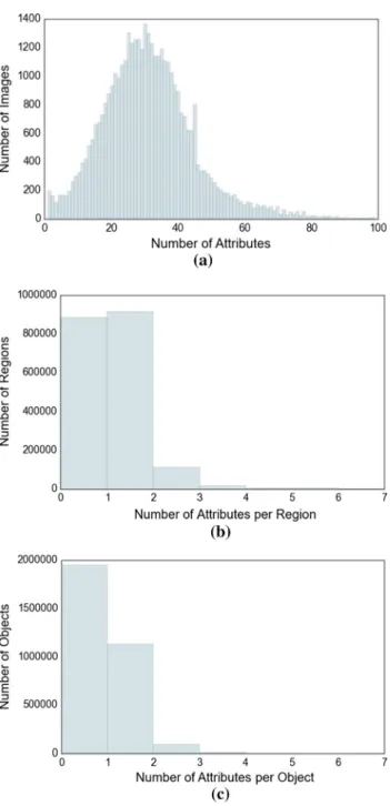
Each image in Visual Genome has an average of 26 attributes. Objects can have zero or more attributes
asso-Fig. 6 From all of the region descriptions, we extract all objects men-tioned. For example, from the region description “man jumpingovera fire hydrant,” we extractmanandfire hydrant
Fig. 7 Some descriptions also provide attributes for objects. For exam-ple, the region description “yellowfire hydrant” adds that thefire hydrant isyellow. Here we show two attributes:yellowand
standing
ciated with them. Attributes can be color (e.g. yellow),
states (e.g. standing), etc. (Fig. 7). Just like we
col-lect objects from region descriptions, we also colcol-lect the
attributes attached to these objects. In Fig. 7, from the
phrase “yellow fire hydrant,” we extract the attributeyellow
for the fire hydrant. As with objects, we
canonical-ize all attributes to WordNet (Miller 1995); for example,
yellowis mapped toyellow.s.01 (of the color intermediate between green and orange in
Fig. 8 Our dataset also captures the relationships and interactions between objects in our images. In this example, we show the relation-shipjumping overbetween the objectsmanandfire hydrant
the color spectrum; of something resembling the color of an egg yolk). 2.4 A Set of Relationships
Relationships connect two objects together. These
relation-ships can be actions (e.g.jumping over), spatial (e.g.is
behind), descriptive verbs (e.g.wear), prepositions (e.g.
with), comparative (e.g.taller than), or prepositional
phrases (e.g. drive on). For example, from the region
description “man jumping over fire hydrant,” we extract the
relationshipjumping overbetween the objectsmanand
fire hydrant(Fig.8). These relationships are directed from one object, called the subject, to another, called the
object. In this case, the subject is theman, who is
perform-ing the relationshipjumping overon the object fire
hydrant. Each relationship is canonicalized to a
Word-Net (Miller 1995) synset ID; i.e. jumping is
canonical-ized tojump.a.1 (move forward by leaps and
bounds). On average, each image in our dataset contains 21 relationships.
2.5 A Set of Region Graphs
Combining the objects, attributes, and relationships extracted from region descriptions, we create a directed graph repre-sentation for each of the regions. Examples of region graphs
are shown in Fig.4. Each region graph is a structured
rep-resentation of a part of the image. The nodes in the graph represent objects, attributes, and relationships. Objects are linked to their respective attributes while relationships link one object to another. The links connecting two objects in
Fig.4point from the subject to the relationship and from the
relationship to the other object.
2.6 One Scene Graph
While region graphs are localized representations of an image, we also combine them into a single scene graph
rep-resenting the entire image (Fig.3). The scene graph is the
unionof all region graphs and contains all objects, attributes, and relationships from each region description. By doing so, we are able to combine multiple levels of scene information
in a more coherent way. For example in Fig.4, the leftmost
region description tells us that the “fire hydrant is yellow,” while the middle region description tells us that the “man is jumping over the fire hydrant.” Together, the two descriptions tell us that the “man is jumping over a yellow fire hydrant.”
2.7 A Set of Question Answer Pairs
We have two types of QA pairs associated with each image
in our dataset:freeform QAs, based on the entire image, and
region-based QAs, based on selected regions of the image.
We collect 6 different types of questions per image:what,
where,how,when,who, andwhy. In Fig.4, “Q. What is the woman standing next to?; A. Her belongings” is a freeform QA. Each image has at least one question of each type listed above. Region-based QAs are collected by prompt-ing workers with region descriptions. For example, we use the region “yellow fire hydrant” to collect the region-based QA: “Q. What color is the fire hydrant?; A. Yellow.” Region based QAs are based on the description and allow us to independently study how well models perform at answer-ing questions usanswer-ing the image or the region description as input.
3 Related Work
We discuss existing datasets that have been released and used by the vision community for classification and object detec-tion. We also mention work that has improved object and attribute detection models. Then, we explore existing work that has utilized representations similar to our relationships between objects. In addition, we dive into literature related to cognitive tasks like image description, question answering, and knowledge representation.
3.1 Datasets
Datasets (Table1) have been growing in size as researchers
have begun tackling increasingly complicated problems.
Cal-tech 101(Fei-Fei et al. 2007) was one of the first datasets hand-curated for image classification, with 101 object
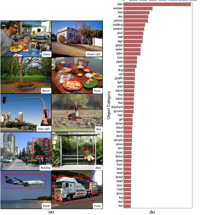
cate-Ta b le 1 A comparison o f existing d atasets w ith V isual G enome Images Descriptions per image T o tal objects # Object cate gories Objects p er image # A ttrib u tes cate gories Attrib utes per image # R elationship cate gories Relationships per image Question answers YFCC100M ( Thomee et al. 2016 ) 100,000,000 – – – –––– –– T in y images ( T o rralba et al. 2008 ) 80,000,000 – – 53,464 1––– –– ImageNet ( Deng et al. 2009 ) 14,197,122 – 14,197,122 21,841 1––– –– ILSVRC detection (2012) ( Russak o vsk y et al. 2015 ) 476,688 – 534,309 200 2.5 – – – – – MS-COCO ( Lin et al. 2014 ) 328,000 5 27,472 80 –––– –– Flickr 30K ( Y oung et al. 2014 ) 3 1 ,7 8 3 5–––––– –– Caltech 101 ( Fei-Fei et al. 2007 ) 9144 – 9144 102 1––– –– Caltech 256 ( Grif fin et al. 2007 ) 3 0 ,6 0 8 –3 0 ,6 0 8 2 5 7 1––– –– Caltech pedestrian ( Dollar et al. 2012 ) 250,000 – 350,000 1 1 .4 – – – – – P ascal detection ( Ev eringham et al. 2010 ) 11,530 – 27,450 20 2.38 – – – – – Abstract scenes ( Zitnick and P arikh 2013 ) 1 0 ,0 2 0 –5 8 1 1 5––– –– aP ascal ( F arhadi et al. 2009 ) 12,000 – – – – 6 4 – – – – Animal attrib utes ( Lampert et al. 2009 ) 30,000 – – – – 1 ,280 – – – – SUN attrib u tes ( P atterson et al. 2014 ) 14,000 – – – – 700 700 – – – Caltech birds ( W ah et al. 2011 ) 11,788 – – – – 312 312 – – – COCO actions ( Ronchi and P erona 2015 ) 10,000 – – – 5.2 – – 156 20.7 – V isual phrases ( Sade ghi and F arhadi 2011 ) – ––––––1 7 1 – Vi sK E ( Sade ghi et al. 2015 ) – – – – – – – 6500 – – DA Q U A R ( Malino wski and F ritz 2014 ) 1 ,4 4 9 ––––––– –1 2 ,4 6 8 COCO QA ( Ren et al. 2015a ) 123,287 – – – –––– – 117,684 Baidu ( Gao et al. 2015 ) 120,360 – – – –––– – 250,569 VQA ( Antol et al. 2015 ) 204,721 – – – –––– – 614,163 V isual Genome 108,077 50 3,843,636 33,877 35 68,111 26 42,374 21 1,773,258 W e sho w that V isual Genome h as an order o f m agnitude more descriptions and question answers. It also h as a m ore d iv erse set o f object, attrib ute, and rel ationship classes. Additionally , V isual Genome contains a h igher d ensity of these annotations per image. T he number o f d istinct cate gories in V isual G enome are calculated b y lo w er -casing an d stemming n ames of objects, attrib utes and relationships
gories and 15–30 examples per category. One of the biggest criticisms of Caltech 101 was the lack of variability in its
examples.Caltech 256 (Griffin et al. 2007) increased the
number of categories to 256, while also addressing some of the shortcomings of Caltech 101. However, it still had only a handful of examples per category, and most of its
images contained only a single object. LabelMe (Russell
et al. 2008) introduced a dataset with multiple objects per category. They also provided a web interface that experts and novices could use to annotate additional images. This web interface enabled images to be labeled with polygons,
helping create datasets for image segmentation. TheLotus
Hill dataset(Yao et al. 2007) contains a hierarchical decom-position of objects (vehicles, man-made objects, animals, etc.) along with segmentations. Only a small part of this
dataset is freely available.SUN (Xiao et al. 2010), just like
LabelMe (Russell et al. 2008) and Lotus Hill (Yao et al. 2007), was curated for object detection. Pushing the size
of datasets even further, 80Million Tiny Images(Torralba
et al. 2008) created a significantly larger dataset than its
predecessors. It contains tiny (i.e. 32×32 pixels) images
that were collected using WordNet (Miller 1995) synsets as queries. However, because the data in 80 Million Images were not human-verified, they contain numerous errors. YFCC100M(Thomee et al. 2016) is another large database of 100 million images that is still largely unexplored. It contains human generated and machine generated tags.
Pascal VOC (Everingham et al. 2010) pushed research from classification to object detection with a dataset
con-taining 20 semantic categories in 11,000 images.
Ima-geNet(Deng et al. 2009) took WordNet synsets and crowd-sourced a large dataset of 14 million images. They started the ILSVRC (Russakovsky et al. 2015) challenge for a variety of computer vision tasks. Together, ILSVRC and PASCAL pro-vide a test bench for object detection, image classification, object segmentation, person layout, and action classification. MS-COCO (Lin et al. 2014) recently released its dataset,
with over 328,000 images with sentence descriptions and
segmentations of 80 object categories. The previous largest
dataset for image-based QA,VQA(Antol et al. 2015),
con-tains 204,721 images annotated with three question answer pairs. They collected a dataset of 614,163 freeform questions
with 6.1M ground truth answers (10 per question) and
pro-vided a baseline approach in answering questions using an image and a textual question as the input.
Visual Genomeaims to bridge the gap between all these datasets, collecting not just annotations for a large number of objects but also scene graphs, region descriptions, and question answer pairs for image regions. Unlike previous datasets, which were collected for a single task like image classification, the Visual Genome dataset was collected to be a general-purpose representation of the visual world, without bias toward a particular task. Our images contain an average
of 35 objects, which is almost an order of magnitude more dense than any existing vision dataset. Similarly, we contain an average of 26 attributes and 21 relationships per image. We also have an order of magnitude more unique objects, attributes, and relationships than any other dataset. Finally,
we have 1.7 million question answer pairs, also larger than
any other dataset for visual question answering.
3.2 Image Descriptions
One of the core contributions of Visual Genome is its descrip-tions for multiple regions in an image. As such, we mention other image description datasets and models in this subsec-tion. Most work related to describing images can be divided into two categories: retrieval of human-generated captions and generation of novel captions. Methods in the first cat-egory use similarity metrics between image features from predefined models to retrieve similar sentences (Ordonez et al. 2011;Hodosh et al. 2013). Other methods map both sen-tences and their images to a common vector space (Ordonez et al. 2011) or map them to a space of triples (Farhadi et al. 2010). Among those in the second category, a common theme has been to use recurrent neural networks to produce novel
captions (Kiros et al. 2014;Mao et al. 2014;Karpathy and
Fei-Fei 2015;Vinyals et al. 2015;Chen and Lawrence Zitnick 2015;Donahue et al. 2015;Fang et al. 2015). More recently, researchers have also used a visual attention model (Xu et al. 2015).
One drawback of these approaches is their attention to describing only the most salient aspect of the image. This problem is amplified by datasets like Flickr 30K (Young et al. 2014) and MS-COCO (Lin et al. 2014), whose sen-tence desriptions tend to focus, somewhat redundantly, on these salient parts. For example, “an elephant is seen wan-dering around on a sunny day,” “a large elephant in a tall grass field,” and “a very large elephant standing alone in some brush” are 3 descriptions from the MS-COCO dataset, and all of them focus on the salient elephant in the image and ignore the other regions in the image. Many real-world scenes are complex, with multiple objects and interactions that are best described using multiple descriptions (Karpa-thy and Fei-Fei 2015;Lebret et al. 2015). Our dataset pushes toward a more complete understanding of an image by col-lecting a dataset in which we capture not just scene-level descriptions but also myriad of low-level descriptions, the “grammar” of the scene.
3.3 Objects
Object detection is a fundamental task in computer vision, with applications ranging from identification of faces in photo software to identification of other cars by self-driving cars on the road. It involves classifying an object into a
dis-tinct category and localizing the object in the image. Visual Genome uses objects as a core component on which each visual scene is built. Early datasets include the face detec-tion (Huang et al. 2008) and pedestrian datasets (Dollar et al. 2012). The PASCAL VOC and ILSVRC’s detection dataset pushed research in object detection. But the images in these datasets are iconic and do not capture the settings in which these objects usually co-occur. To remedy this problem, MS-COCO (Lin et al. 2014) annotated real-world scenes that capture object contexts. However, MS-COCO was unable to describe all the objects in its images, since they annotated only 80 object categories. In the real world, there are many more objects that the ones captured by existing datasets. Visual Genome aims at collecting annotations for all visual elements that occur in images, increasing the number of
dis-tinct categories to 33,877.
3.4 Attributes
The inclusion of attributes allows us to describe, compare, and more easily categorize objects. Even if we haven’t seen an object before, attributes allow us to infer something about it; for example, “yellow and brown spotted with long neck” likely refers to a giraffe. Initial work in this area involved find-ing objects with similar features (Malisiewicz et al. 2008) using examplar SVMs. Next, textures were used to study objects (Varma and Zisserman 2005), while other meth-ods learned to predict colors (Ferrari and Zisserman 2007). Finally, the study of attributes was explicitly demonstrated to lead to improvements in object classification (Farhadi et al. 2009). Attributes were defined to be parts (e.g. “has legs”), shapes (e.g. “spherical”), or materials (e.g. “furry”) and could be used to classify new categories of objects. Attributes have also played a large role in improving fine-grained recogni-tion (Goering et al. 2014) on fine-grained attribute datasets like CUB-2011 (Wah et al. 2011). In Visual Genome, we use a generalized formulation (Johnson et al. 2015), but we extend it such that attributes are not image-specific bina-ries but rather object-specific for each object in a real-world scene. We also extend the types of attributes to include size (e.g. “small”), pose (e.g. “bent”), state (e.g. “transparent”), emotion (e.g. “happy”), and many more.
3.5 Relationships
Relationship extraction has been a traditional problem in information extraction and in natural language
process-ing. Syntactic features (Zhou et al. 2007; GuoDong et al.
2005), dependency tree methods (Culotta and Sorensen 2004; Bunescu and Mooney 2005), and deep neural
net-works (Socher et al. 2012; Zeng et al. 2014) have been
employed to extract relationships between two entities in a sentence. However, in computer vision, very little work has
gone into learning or predicting relationships. Instead, rela-tionships have been implicitly used to improve other vision tasks. Relative layouts between objects have improved scene categorization (Izadinia et al. 2014), and 3D spatial geome-try between objects has helped object detection (Choi et al. 213). Comparative adjectives and prepositions between pairs of objects have been used to model visual relationships and improved object localization (Gupta and Davis 2008).
Relationships have already shown their utility in
improv-ing visual cognitive tasks (Antol et al. 2014; Yang et al.
2012). A meaning space of relationships has improved the mapping of images to sentences (Farhadi et al. 2010). Rela-tionships in a structured representation with objects have
been defined as a graph structure called ascene graph, where
the nodes are objects with attributes and edges are relation-ships between objects. This representation can be used to generate indoor images from sentences and also to improve
image search (Chang et al. 2014;Johnson et al. 2015). We
use a similar scene graph representation of an image that generalizes across all these previous works (Johnson et al. 2015). Recently, relationships have come into focus again in the form of question answering about associations between objects (Sadeghi et al. 2015). These questions ask if a rela-tionship, involving generally two objects, is true, e.g. “do dogs eat ice cream?”. We believe that relationships will be necessary for higher-level cognitive tasks (Johnson et al. 2015; Lu et al. 2016), so we collect the largest corpus of them in an attempt to improve tasks by actually understand-ing interactions between objects.
3.6 Question Answering
Visual question answering (QA) has been recently proposed as a proxy task of evaluating a computer vision system’s ability to understand an image beyond object recognition
and image captioning (Geman et al. 2015;Malinowski and
Fritz 2014). Several visual QA benchmarks have been pro-posed in the last few months. The DAQUAR (Malinowski and Fritz 2014) dataset was the first toy-sized QA bench-mark built upon indoor scene RGB-D images of NYU Depth v2 (Nathan Silberman and Fergus 2012). Most new
datasets (Yu et al. 2015;Ren et al. 2015a;Antol et al. 2015;
Gao et al. 2015) have collected QA pairs on MS-COCO images, either generated automatically by NLP tools (Ren et al. 2015a) or written by human workers (Yu et al. 2015; Antol et al. 2015;Gao et al. 2015).
In previous datasets, most questions concentrated on sim-ple recognition-based questions about the salient objects, and answers were often extremely short. For instance, 90% of DAQUAR answers (Malinowski and Fritz 2014) and 89% of VQA answers (Antol et al. 2015) consist of single-word object names, attributes, and quantities. This limitation bounds their diversity and fails to capture the long-tail details
of the images. Given the availability of new datasets, an array of visual QA models have been proposed to tackle QA tasks. The proposed models range from SVM classifiers and prob-abilistic inference (Malinowski and Fritz 2014) to recurrent
neural networks (Gao et al. 2015;Malinowski et al. 2015;Ren
et al. 2015a) and convolutional networks (Ma et al. 2015). Visual Genome aims to capture the details of the images with diverse question types and long answers. These questions should cover a wide range of visual tasks from basic
percep-tion to complex reasoning. Our QA dataset of 1.7 million
QAs is also larger than any currently existing dataset.
3.7 Knowledge Representation
A knowledge representation of the visual world is capable of tackling an array of vision tasks, from action recogni-tion to general quesrecogni-tion answering. However, it is difficult to answer “what is the minimal viable set of knowledge needed to understand about the physical world?” (Hayes 1978). It was later proposed that there be a certain plurality to concepts and their related axioms (Hayes 1985). These efforts have grown to model physical processes (Forbus 1984) or to model a series of actions as scripts (Schank and Abelson 2013) for stories—both of which are not depicted in a single static image but which play roles in an image’s story (Vedantam et al. 2015b). More recently, NELL (Betteridge et al. 2009) learns probabilistic horn clauses by extracting information from the web. DeepQA (Ferrucci et al. 2010) proposes a probabilistic question answering architecture involving over 100 different techniques. Others have used Markov logic
networks (Zhu et al. 2009;Niu et al. 2012) as their
repre-sentation to perform statistical inference for knowledge base construction. Our work is most similar to that of those (Chen et al. 2013;Zhu et al. 2014,2015;Sadeghi et al. 2015) who attempt to learn common-sense relationships from images.
Visual Genome scene graphs can also be considered adense
knowledge representation for images. It is similar to the for-mat used in knowledge bases in NLP.
4 Crowdsourcing Strategies
Visual Genome was collected and verified entirely by crowd workers from Amazon Mechanical Turk. In this section, we outline the pipeline employed in creating all the components of the dataset. Each component (region descriptions, objects, attributes, relationships, region graphs, scene graphs, ques-tions and answers) involved multiple task stages. We mention the different strategies used to make our data accurate and to enforce diversity in each component. We also provide background information about the workers who helped make Visual Genome possible.
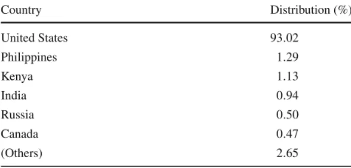
Table 2 Geographic distribution of countries from where crowd work-ers contributed to Visual Genome
Country Distribution (%) United States 93.02 Philippines 1.29 Kenya 1.13 India 0.94 Russia 0.50 Canada 0.47 (Others) 2.65 4.1 Crowd Workers
We used Amazon Mechanical Turk (AMT) as our primary
source of annotations. Overall, a total of over 33,000 unique
workers contributed to the dataset. The dataset was collected over the course of 6 months after 15 months of experimenta-tion and iteraexperimenta-tion on the data representaexperimenta-tion. Approximately
800,000 Human Intelligence Tasks (HITs) were launched on
AMT, where each HIT involved creating descriptions, ques-tions and answers, or region graphs. Each HIT was designed such that workers manage to earn anywhere between $6-$8 per hour if they work continuously, in line with ethical research standards on Mechanical Turk (Salehi et al. 2015).
Visual Genome HITs achieved a 94.1% retention rate,
mean-ing that 94.1% of workers who completed one of our tasks
went ahead to do more. Table2outlines the percentage
dis-tribution of the locations of the workers. 93.02% of workers
contributed from the United States.
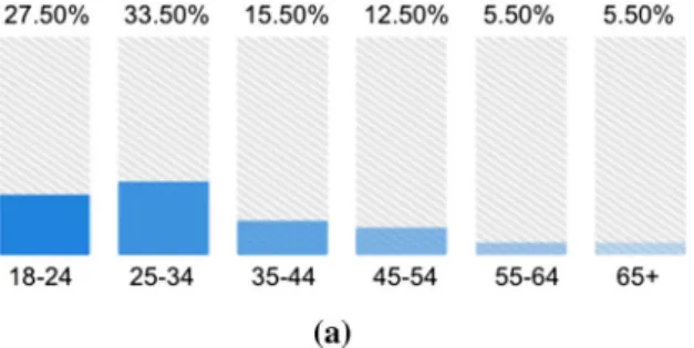
Figure9a, b outline the demographic distribution of our
crowd workers. This data was collected using a survey HIT. The majority of our workers were between the ages of 25 and 34 years old. Our youngest contributor was 18 years and the oldest was 68 years old. We also had a near-balanced split of
54.15% male and 45.85% female workers.
4.2 Region Descriptions
Visual Genome’s main goal is to enable the study of cognitive computer vision tasks. The next step towards understand-ing images requires studyunderstand-ing relationships between objects in scene graph representations of images. However, we observed that collecting scene graphs directly from an image leads to workers annotating easy, frequently-occurring
rela-tionships like wearing(man,shirt) instead of focusing on
salient parts of the image. This is evident from previous
datasets (Johnson et al. 2015; Lu et al. 2016) that contain
a large number of such relationships. After experimentation, we observed that when asked to describe an image using nat-ural language, crowd workers natnat-urally start with the most salient part of the image and then move to describing other
Fig. 9 aAge andbgender distribution of Visual Genome’s crowd workers parts of the image one by one. Inspired by this finding, we focused our attention towards collecting a dataset of region descriptions that is diverse in content.
When a new image is added to the crowdsourcing pipeline with no annotations, it is sent to a worker who is asked to draw three bounding boxes and write three descriptions for the region enclosed by each box. Next, the image is sent to another worker along with the previously written descrip-tions. Workers are explicitly encouraged to write descriptions that have not been written before. This process is repeated until we have collected 50 region descriptions for each image. To prevent workers from having to skim through a long list of previously written descriptions, we only show them the top seven most similar descriptions. We calculate these most similar descriptions using BLEU-like (Papineni et al. 2002) (n-gram) scores between pairs of sentences. We define the
similarity scoreS between a descriptiondi and a previous
descriptiondj to be: Sn(di,dj)=b(di,dj)exp 1 N N n=1 logpn(di,dj) (1)
where we enforce a brevity penalty using:
b(di,dj)= 1 iflen(di) >len(dj) e1− len(d j) len(di) otherwise (2)
andpncalculates the percentage of n-grams indithat match
n-grams indj.
When a worker writes a new description, we programmat-ically enforce that it has not been repeated by using BLEU
score thresholds set to 0.7 to ensure that it is dissimilar to
descriptions from both of the following two lists:
1. Image-Specific Descriptions A list of all previously written descriptions for that image.
2. Global Image DescriptionsA list of the top 100 most common written descriptions of all images in the dataset. This prevents very common phrases like “sky is blue”
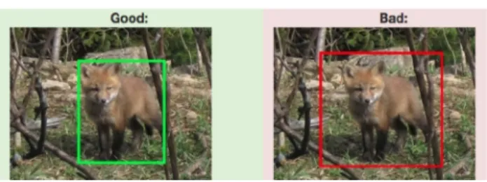
Fig. 10 Good (left) and bad (right) bounding boxes for the phrase “a street with aredcar parked on the side,” judged oncoverage
from dominating the set of region descriptions. The list of top 100 global descriptions is continuously updated as more data comes in.
Finally, we ask workers to draw bounding boxes that
sat-isfy one requirement: coverage. The bounding box must
cover all objects mentioned in the description. Figure 10
shows an example of a good box that covers both thestreet
as well thecarmentioned in the description, as well as an
example of a bad box.
4.3 Objects
Once 50 region descriptions are collected for an image, we extract the visual objects from each description. Each description is sent to one crowd worker, who extracts all the objects from the description and grounds each object as a
bounding box in the image. For example, from Fig.4, let’s
consider the description “woman in shorts is standing behind
the man.” A worker would extract three objects: woman,
shorts, andman. They would then draw a box around each of the objects. We require each bounding box to be drawn
to satisfy two requirements:coverageandquality.
Cover-age has the same definition as described above in Sect.4.2,
where we ask workers to make sure that the bounding box
covers the object completely (Fig.11). Quality requires that
each bounding box be as tight as possible around its object such that if the box’s length or height were decreased by one pixel, it would no longer satisfy the coverage requirement.
Fig. 11 Good (left) and bad (right) bounding boxes for the objectfox, judged on bothcoverageas well asquality
Since a one pixel error can be physically impossible for most workers, we relax the definition of quality to four pixels.
Multiple descriptions for an image might refer to the same
object, sometimes with different words. For example, aman
in one description might be referred to aspersonin another
description. We can thus use this crowdsourcing stage to build these co-reference chains. With each region description given to a worker to process, we include a list of previously extracted objects as suggestions. This allows a worker to
choose a previously drawn box annotated asmaninstead of
redrawing a new box forperson.
Finally, to increase the speed with which workers com-plete this task, we also use Stanford’s dependency parser (Manning et al. 2014) to extract nouns automatically and send them to the workers as suggestions. While the parser manages to find most of the nouns, it sometimes misses compound nouns, so we avoided completely depending on this auto-mated method. By combining the parser with crowdsourcing tasks, we were able to speed up our object extraction process without losing accuracy.
4.4 Attributes, Relationships, and Region Graphs Once all objects have been extracted from each region description, we can extract the attributes and relationships described in the region. We present each worker with a region description along with its extracted objects and ask them to add attributes to objects or to connect pairs of objects with relationships, based on the text of the description. From the description “woman in shorts is standing behind the man”,
workers will extract the attributestandingfor thewoman
and the relationshipsin(woman,shorts) andbehind(woman,
man). Together, objects, attributes, and relationships form
the region graph for a region description. Some descriptions like “it is a sunny day” do not contain any objects and there-fore have no region graphs associated with them. Workers are asked to not generate any graphs for such descriptions. We create scene graphs by combining all the region graphs for an image by combining all the co-referenced objects from different region graphs.
Fig. 12 Each object (fox) has only one bounding box referring to it (left). Multiple boxes drawn for the same object (right) are combined together if they have a minimum threshold of 0.9 intersection over union
4.5 Scene Graphs
The scene graph is the union of all region graphs extracted from region descriptions. We merge nodes from region
graphs that correspond to the same object; for example,man
andpersonin two different region graphs might refer to the same object in the image. We say that objects from dif-ferent graphs refer to the same object if their bounding boxes
have an intersection over union of 0.9. However, this
heuris-tic might contain false positives. So, before merging two objects, we ask workers to confirm that a pair of objects with significant overlap are indeed the same object. For
exam-ple, in Fig. 12 (right), the fox might be extracted from
two different region descriptions. These boxes are then
com-bined together (Fig. 12, left) when constructing the scene
graph.
4.6 Questions and Answers
To create question answer (QA) pairs, we ask the AMT work-ers to write pairs of questions and answwork-ers about an image. To ensure quality, we instruct the workers to follow three rules:
1) start the questions with one of the “six Ws” (who,what,
where,when,whyandhow); 2) avoid ambiguous and spec-ulative questions; 3) be precise and unique, and relate the question to the image such that it is clearly answerable if and only if the image is shown.
We collected two separate types of QAs: freeform QAs and region-based QAs. In freeform QA, we ask a worker to look at an image and write eight QA pairs about it. To encourage diversity, we enforce that workers write at least three different Ws out of the six in their eight pairs. In region-based QA, we ask the workers to write a pair region-based on a given region. We select the regions that have large areas (more than 5k pixels) and long phrases (more than 4 words). This enables us to collect around twenty region-based pairs at the same cost of the eight freeform QAs. In general, freeform QA tends to yield more diverse QA pairs that enrich the question distribution; region-based QA tends to produce more factual QA pairs at a lower cost.
4.7 Verification
All Visual Genome data go through a verification stage as soon as they are annotated. This stage helps eliminate incor-rectly labeled objects, attributes, and relationships. It also helps remove region descriptions and questions and answers that might be correct but are vague (“This person seems to enjoy the sun.”), subjective (“room looks dirty”), or opinion-ated (“Being exposed to hot sun like this may cause cancer”). Verification is conducted using two separate strategies: majority voting (Snow et al. 2008) and rapid judgments (Krishna et al. 2016). All components of the dataset except objects are verified using majority voting. Majority vot-ing(Snow et al. 2008) involves three unique workers looking at each annotation and voting on whether it is factually cor-rect. An annotation is added to our dataset if at least two (a majority) out of the three workers verify that it is correct.
We only use rapid judgments to speed up the verification of the objects in our dataset. Rapid judgments (Krishna et al. 2016) use an interface inspired by rapid serial visual pro-cessing that enable verification of objects with an order of magnitude increase in speed than majority voting.
4.8 Canonicalization
All the descriptions and QAs that we collect are freeform worker-generated texts. They are not constrained by any lim-itations. For example, we do not force workers to refer to a
man in the image as aman. We allow them to choose to refer
to the man asperson,boy,man, etc. This ambiguity makes
it difficult to collect all instances ofmanfrom our dataset. In
order to reduce the ambiguity in the concepts of our dataset and connect it to other resources used by the research commu-nity, we map all objects, attributes, relationships, and noun phrases in region descriptions and QAs to synsets in
Word-Net (Miller 1995). In the example above, person,boy,
and man would map to the synsets:person.n.01 (a
human being),male_child.n.01 (a youthful male person)andman.n.03 (the generic use of the word to refer to any human being)
respectively. Thanks to the WordNet hierarchy it is now pos-sible to fuse those three expressions of the same concept into
person.n.01 (a human being), which is the low-est common anclow-estor node of all aforementioned synsets.
We use the Stanford NLP tools (Manning et al. 2014) to extract the noun phrases from the region descriptions and QAs. Next, we map them to their most frequent matching synset in WordNet according to WordNet lexeme counts. We then refine this simple heuristic by hand-crafting mapping rules for the 30 most common failure cases. For example according to WordNet’s lexeme counts the most common
semantic for “table” istable.n.01 (a set of data
arranged in rows and columns). However in our
data it is more likely to see pieces of furniture and therefore
bias the mapping towardstable.n.02 (a piece of
furniture having a smooth flat top that is usually supported by one or more vertical legs). The objects in our scene graphs are already noun phrases and are mapped to WordNet in the same way.
We normalize each attribute based on morphology (so called “stemming”) and map them to the WordNet adjectives. We include 15 hand-crafted rules to address common failure cases, which typically occur when the concrete or spatial sense of the word seen in an image is not the most common
overall sense. For example, the synset long.a.02 (of
relatively great or greater than average spatial extension)is less common in WordNet than
long.a.01 (indicating a relatively great or greater than average duration of time), even though instances of the word “long” in our images are much more likely to refer to that spatial sense.
For relationships, we ignore all prepositions as they are not recognized by WordNet. Since the meanings of verbs are highly dependent upon their morphology and syntactic place-ment (e.g. passive cases, prepositional phrases), we try to find WordNet synsets whose sentence frames match with the context of the relationship. Sentence frames in WordNet are formalized syntactic frames in which a certain sense of a word
might appear; e.g. , play.v.01: participate in
games or sportoccurs in the sentence frames “Some-body [play]s” and “Some“Some-body [play]s something.” For each verb-synset pair, we then consider the root hypernym of that synset to reduce potential noise from WordNet’s fine-grained sense distinctions. The WordNet hierarchy for verbs is seg-mented and originates from over 100 root verbs. For example,
draw.v.01: cause to move by pulling traces
back to the root hypernym move.v.02: cause to
move or shift into a new position, while
draw.v.02: get or derivetraces to the rootget. v.01: come into the possession of some thing concrete or abstract. We also include 20 hand-mapped rules, again to correct for WordNet’s lower representation of concrete or spatial senses.
These mappings are not perfect and still contain some ambiguity. Therefore, we send all our mappings along with the top four alternative synsets for each term to AMT. We ask workers to verify that our mapping was accurate and change the mapping to an alternative one if it was a better fit. We present workers with the concept we want to canonicalize along with our proposed corresponding synset with 4 addi-tional options. To prevent workers from always defaulting to the our proposed synset, we do not explicitly specify which one of the 5 synsets presented is our proposed synset.
Sec-tion5.8provides experimental precision and recall scores for
5 Dataset Statistics and Analysis
In this section, we provide statistical insights and analysis for each component of Visual Genome. Specifically, we
exam-ine the distribution ofimages (Sect.5.1) and the collected
data forregion descriptions (Sect. 5.2) and questions and
answers(Sect. 5.7). We analyze region graphs and scene graphstogether in one section (Sect.5.6), but we also break up these graph structures into their three constituent parts— objects(Sect.5.3),attributes(Sect.5.4), andrelationships
(Sect. 5.5)—and study each part individually. Finally, we
describe our canonicalization pipeline and results (Sect.5.8).
5.1 Image Selection
The Visual Genome dataset consists of all 108,077 creative
commons images from the intersection of MS-COCO’s (Lin et al. 2014) 328,000 images and YFCC100M’s (Thomee et al. 2016) 100 million images. This allows Visual Genome annotations to be utilized together with the YFCC tags and MS-COCO’s segmentations and full image captions. These images are real-world, non-iconic images that were uploaded onto Flickr by users. The images range from as small as 72 pixels wide to as large as 1280 pixels wide, with an aver-age width of 500 pixels. We collected the WordNet synsets
into which our 108,077 images can be categorized using the
same method as ImageNet (Deng et al. 2009). Visual Genome images can be categorized into 972 ImageNet synsets. Note that objects, attributes and relationships are categorized
sep-arately into more than 18K WordNet synsets (Sect. 5.8).
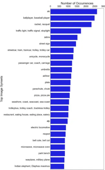
Figure13shows the top synsets to which our images belong.
“ski” is the most common synset, with 2612 images; it is followed by “ballplayer” and “racket,” with all three synsets referring to images of people playing sports. Our dataset is
somewhat biased towards images of people, as Fig.13shows;
however, they are quite diverse overall, as the top 25 synsets each have over 800 images, while the top 50 synsets each have over 500 examples.
5.2 Region Description Statistics
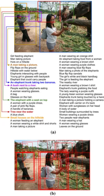
One of the primary components of Visual Genome is its region descriptions. Every image includes an average of 50 regions with a bounding box and a descriptive phrase.
Figure14shows an example image from our dataset with its
50 region descriptions. We display bounding boxes for only 6 out of the 50 descriptions in the figure to avoid clutter. These descriptions tend to be highly diverse and can focus on a single object, like in “A bag,” or on multiple objects, like in “Man taking a photo of the elephants.” They encompass the most salient parts of the image, as in “An elephant taking food from a woman,” while also capturing the background, as in “Small buildings surrounded by trees.”
Fig. 13 A distribution of the top 25 image synsets in the Visual Genome dataset. A variety of synsets are well represented in the dataset, with the top 25 synsets having at least 800 example images each. Note that an image synset is the label of the entire image according to the Ima-geNet ontology and are separate from the synsets for objects, attributes and relationships
MS-COCO (Lin et al. 2014) dataset is good at generat-ing variations on a sgenerat-ingle scene-level descriptor. Consider three sentences from MS-COCO dataset on a similar image: “there is a person petting a very large elephant,” “a per-son touching an elephant in front of a wall,” and “a man in white shirt petting the cheek of an elephant.” These three sentences are single scene-level descriptions. In comparison, Visual Genome descriptions emphasize different regions in the image and thus are less semantically similar. To ensure diversity in the descriptions, we use BLEU score (Pap-ineni et al. 2002) thresholds between new descriptions and all previously written descriptions. More information about
crowdsourcing can be found in Sect.4.
Region descriptions must be specific enough in an image to describe individual objects (e.g. “A bag”), but they must also be general enough to describe high-level concepts in an
Fig. 14 aAn example image from the dataset with its region descrip-tions. We only display localizations for 6 of the 50 descriptions to avoid clutter; all 50 descriptions do have corresponding bounding boxes.b All 50 region bounding boxes visualized on the image
image (e.g. “A man being chased by a bear”). Qualitatively, we note that regions that cover large portions of the image tend to be general descriptions of an image, while regions that cover only a small fraction of the image tend to be more
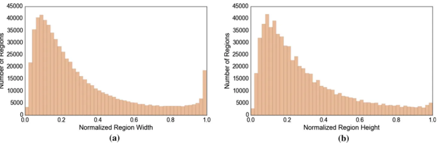
specific. In Fig.15a, we show the distribution of regions over
the width of the region normalized by the width of the image. We see that the majority of our regions tend to be around 10 to 15% of the image width. We also note that there are a large number of regions covering 100% of the image width. These regions usually include elements like “sky,” “ocean,” “snow,” “mountains,” etc. that cannot be bounded and thus span the
entire image width. In Fig.15b, we show a similar distribution
over the normalized height of the region. We see a similar overall pattern, as most of our regions tend to be very specific descriptions of about 10% to 15% of the image height. Unlike the distribution over width, however, we do not see a increase in the number of regions that span the entire height of the image, as there are no common visual equivalents that span images vertically. Out of all the descriptions gathered, only one or two of them tend to be global scene descriptions that
are similar to MS-COCO (Lin et al. 2014) (Fig.17).
In Fig.16, we show the distribution of the length (word
count) of these region descriptions. The average word count for a description is 5 words, with a minimum of 1 and a
max-imum of 12 words. In Fig.18a, we plot the most common
phrases occurring in our region descriptions, with common stop words removed. Common visual elements like “green grass,” “tree [in] distance,” and “blue sky” occur much more often than other, more nuanced elements like “fresh straw-berry.” We also study descriptions with finer precision in Fig.18b, where we plot the most common words used in descriptions. Again, we eliminate stop words from our study. Colors like “white” and “black” are the most frequently used words to describe visual concepts; we conduct a similar study on other captioning datasets including MS-COCO (Lin et al. 2014) and Flickr 30K (Young et al. 2014) and find a similar distribution with colors occurring most frequently. Besides colors, we also see frequent occurrences of common objects like “man” and “tree” and of universal visual elements like “sky.”
Semantic Diversity We also study the actual semantic con-tents of the descriptions. We use an unsupervised approach to analyze the semantics of these descriptions. Specifically, we use word2vec’s (Mikolov et al. 2013) pre-trained model on Google news corpus to convert each word in a description to a 300-dimensional vector. Next, we remove stop words and average the remaining words to get a vector representation of the whole region description. This pipeline is outlined
in Fig. 17. We use hierarchical agglomerative clustering
(Steinbach et al. 2000) on vector representations of each region description and find 71 semantic and syntactic
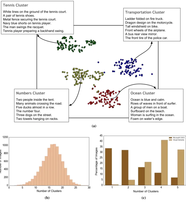
group-ings or “clusters.” Figure 19a shows four such example
clusters. One cluster contains all descriptions related to ten-nis, like “A man swings the racquet” and “White lines on the ground of the tennis court,” while another cluster con-tains descriptions related to numbers, like “Three dogs on the street” and “Two people inside the tent.” To quantitatively measure the diversity of Visual Genome’s region descrip-tions, we calculate the number of clusters represented in a single image’s region descriptions. We show the distribution
of the variety of descriptions for an image in Fig.19b. We
find that on average, each image contains descriptions from 17 different clusters. The image with the least diverse descrip-tions contains descripdescrip-tions from 4 clusters, while the image
Fig. 15 aA distribution of the width of the bounding box of a region description normalized by the image width.bA distribution of the height of the bounding box of a region description normalized by the image height
Fig. 16 A distribution of the number of words in a region description. The average number of words in a region description is 5, with shortest descriptions of 1 word and longest descriptions of 16 words
with the most diverse descriptions contains descriptions from 26 clusters.
Finally, we also compare the descriptions in Visual Genome to the captions in MS-COCO. First we aggregate all Visual Genome and MS-COCO descriptions and remove all stop words. After removing stop words, the descriptions from both datasets are roughly the same length. We conduct a similar study, in which we vectorize the descriptions for each image and calculate each dataset’s cluster diversity per image. We find that on average, 2 clusters are represented in the captions for each image in MS-COCO, with very few images in which 5 clusters are represented. Because each image in MS-COCO only contains 5 captions, it is not a fair comparison to compare the number of clusters represented in all the region descriptions in the Visual Genome dataset. We thus randomly sample 5 Visual Genome region descrip-tions per image and calculate the number of clusters in an image. We find that Visual Genome descriptions come from
4 or 5 clusters. We show our comparison results in Fig.19c.
The difference between the semantic diversity between the
Fig. 17 The process used to convert a region description into a 300-dimensional vectorized representation
two datasets is statistically significant (t = −240,p<0.01)
(Fig.20).
5.3 Object Statistics
In comparison to related datasets, Visual Genome fares
well in terms of object density and diversity (Table 3).
Visual Genome contains approximately 35 objects per image, exceeding ImageNet (Deng et al. 2009), PASCAL (Everingham et al. 2010), MS-COCO (Lin et al. 2014), and
other datasets by large margins. As shown in Fig.21, there
are more object categories represented in Visual Genome than in any other dataset. This comparison is especially per-tinent with regards to Microsoft MS-COCO (Lin et al. 2014), which uses the same images as Visual Genome. The lower count of objects per category is a result of our higher number of categories. For a fairer comparison with ILSVRC 2014 Detection (Russakovsky et al. 2015), Visual Genome has about 2239 objects per category when only the top 200 cat-egories are considered, which is comparable to ILSVRC’s
2671.5 objects per category. For a fairer comparison with
cat-Fig. 18 aA plot of the most common visual concepts or phrases that occur in region descriptions. The most common phrases refer to univer-sal visual concepts like “bluesky,” “greengrass,” etc.bA plot of the most frequently used words in region descriptions. Each word is treated
as an individual token regardless of which region description it came from. Colors occur the most frequently, followed by common objects likemananddogand universal visual concepts like “sky”
egory when only the top 80 categories are considered. This is comparable to MS-COCO’s (Lin et al. 2014) object distri-bution.
The 3,843,636 objects in Visual Genome come from a
variety of categories. As shown in Fig.22(b), objects related
Numbers Cluster
Two people inside the tent. Many animals crossing the road. Five ducks almost in a row. The number four.
Three dogs on the street. Two towels hanging on racks.
Tennis Cluster
White lines on the ground of the tennis court. A pair of tennis shoes.
Metal fence securing the tennis court. Navy blue shorts on tennis player. The man swings the racquet.
Tennis player preparing a backhand swing.
Ocean Cluster
Ocean is blue and calm. Rows of waves in front of surfer. A group of men on a boat. Surfboard on the beach. Woman is surfing in the ocean. Foam on water’s edge.
Transportation Cluster
Ladder folded on fire truck. Dragon design on the motorcycle. Tall windshield on bike.
Front wheels of the airplane. A bus rear view mirror. The front tire of the police car.
(a)
(b) (c)
Fig. 19 aExample illustration showing four clusters of region descrip-tions and their overall themes. Other clusters not shown due to limited space.bDistribution of images over number of clusters represented in each image’s region descriptions.cWe take Visual Genome with 5 random descriptions taken from each image and MS-COCO dataset
with all 5 sentence descriptions per image and compare how many clus-ters are represented in the descriptions. We show that Visual Genome’s descriptions are more varied for a given image, with an average of 4 clusters per image, while MS-COCO’s images have an average of 2 clusters per image
scenery are most common; this is consistent with the gen-eral bias in image subject matter in our dataset. Common
objects like man, person, and woman occur especially
frequently with occurrences of 24K, 17K, and 11K. Other objects that also occur in MS-COCO (Lin et al. 2014)
are also well represented with around 5000 instances on
average. Figure 22a shows some examples of objects in
images. Objects in Visual Genome span a diverse set of Wordnet categories like food, animals, and man-made struc-tures.
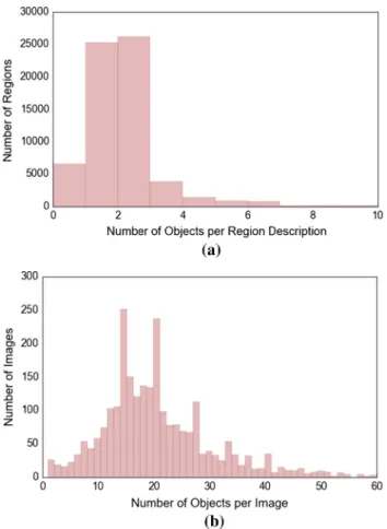
Fig. 20 a Distribution of the number of objects per region. Most regions have between 0 and 2 objects.bDistribution of the number of objects per image. Most images contain between 15 and 20 objects
It is important to look not only at what types of objects we have but also at the distribution of objects in images and
regions. Figure20a shows, as expected, that we have between
0 and 2 objects in each region on average. It is possible for regions to contain no objects if their descriptions refer to no explicit objects in the image. For example, a region described as “it is dark outside” has no objects to extract. Regions with only one object generally have descriptions that focus on the attributes of a single object. On the other hand, regions with two or more objects generally have descriptions that contain
1,000,000 100,000 10,000 1,000 100 10 1 1 10 100 1000 10,000 100,000 Number of Categories
Instances per Category
COCO
ImageNet Detection Visual Genome
(all objects) PASCAL Detection
Zitnick Abstract Scenes
Caltech 101 Caltech 256
Caltech Pedestrian Visual Genome
(top 80 objects)
Fig. 21 Comparison of object diversity between various datasets. Visual Genome far surpasses other datasets in terms of number of cate-gories. When considering only the top 80 object categories, it contains a comparable number of objects as MS-COCO. Thedashed lineis a visual aid connecting the two Visual Genome data points
both attributes of specific objects and relationships between pairs of objects.
As shown in Fig. 20b, each image contains on average
around 35 distinct objects. Few images have an extremely high number of objects (e.g. over 40). Due to the image biases that exist in the dataset, we have twice as many annotations
formenthan we do ofwomen.
5.4 Attribute Statistics
Attributes allow for detailed description and disambiguation
of objects in our dataset. Our dataset contains 2.8 million total
attributes with 68,111 unique attributes. Attributes include
colors (e.g.green), sizes (e.g. tall), continuous action
verbs (e.g. standing), materials (e.g. plastic), etc.
Each object can have multiple attributes.
On average, each image in Visual Genome contains 26
attributes (Fig. 23). Each region contains on average 1
attribute, though about 34% of regions contain no attribute at all; this is primarily because many regions are
relationship-focused. Figure 24a shows the distribution of the most
common attributes in our dataset. Colors (e.g. white,
green) are by far the most frequent attributes. Also
com-mon are sizes (e.g.large) and materials (e.g. wooden).
Figure 24b shows the distribution of attributes describing
Table 3 Comparison of Visual Genome objects and categories to related datasets Visual Genome ILSVRC det. (Russakovsky et al. 2015) MS-COCO (Lin et al. 2014) Caltech101 (Fei-Fei et al. 2007) Caltech256 (Griffin et al. 2007) PASCAL det. (Everingham et al. 2010) Abstract scenes (Zitnick and Parikh 2013) Images 108,077 476,688 328,000 9144 30,608 11,530 10,020 Total objects 3,843,636 534,309 2,500,000 9144 30,608 27,450 58 Total categories 33,877 200 80 102 257 20 11 Objects per category 113.45 2671.50 27472.50 90 119 1372.50 5.27
Fig. 22 aExamples of objects in Visual Genome. Each object is local-ized in its image with a tightly drawn bounding box.bPlot of the most frequently occurring objects in images. People are the most frequently
occurring objects in our dataset, followed by common objects and visual elements likebuilding,shirt, andsky
people (e.g.man,girls, andperson). The most common
attributes describing people are intransitive verbs
describ-ing their states of motion (e.g.standingandwalking).
Certain sports (e.g.skiing, surfboarding) are
over-represented due to an image bias towards these sports.
Attribute Graphs We also qualitatively analyze the attributes in our dataset by constructing co-occurrence graphs, in which
nodes are unique attributes and edges connect those attributes that describe the same object. For example, if an image
con-tained a “large black dog” (large(dog),black(dog)) and
another image contained a “large yellow cat” (large(cat),
yellow(cat)), its attributes would form an incomplete
graph with edges (large,black) and (large,yellow).
We create two such graphs: one for both the total set of attributes and a second where we consider only objects that