Statistical inference for high-dimensional data via U-statistcs

(1)

c

(2)

STATISTICAL INFERENCE FOR HIGH-DIMENSIONAL DATA VIA U-STATISTICS

BY

RUNMIN WANG

DISSERTATION

Submitted in partial fulfillment of the requirements for the degree of Doctor of Philosophy in Statistics

in the Graduate College of the

University of Illinois at Urbana-Champaign, 2020

Urbana, Illinois

Doctoral Committee:

Professor Xiaofeng Shao, Chair and Director of Research Associate Professor Xiaohui Chen

Assistant Professor Georgios Fellouris Professor Douglas G Simpson

(3)

Abstract

Owing to the advances in the science and technology, there is a surge of interest in high-dimensional data. Many methods developed in low or fixed dimensional setting may not be theoretically valid under this new setting, and sometimes are not even applicable when the dimensionality is larger than the sample size. To circumvent the difficulties brought by the high-dimensionality, we consider to use statistics based methods. In this thesis, we investigate the theoretical properties of U-statistics under the high-dimensional setting, and develop the novel U-U-statistics based methods to three problems.

In the first chapter, we propose a new formulation of self-normalization for inference about the mean of high-dimensional stationary processes by using a U-statistic based approach. Self-normalization has attracted considerable attention in the recent literature of time series analy-sis, but its scope of applicability has been limited to /fixed-dimensional parameters for low-dimensional time series. Our original test statistic is a U-statistic with a trimming parameter to remove the bias caused by weak dependence. Under the framework of nonlinear causal processes, we show the asymptotic normality of our U-statistic with the convergence rate dependent upon the order of the Frobenius norm of the long-run covariance matrix. The self-normalized test statistic is then constructed on the basis of recursive subsampled U-statistics and its limiting null distribution is shown to be a functional of time-changed Brownian motion, which differs from the pivotal limit used in the low-dimensional setting. An interesting phenomenon associated with self-normalization is that it works in the high-dimensional context even if the convergence rate of original test statistic is unknown. We also present applications to testing for bandedness of the covariance matrix and testing for white noise for high-dimensional stationary time series and compare the finite sample performance with existing methods in simulation studies. At the root of our theoretical argu-ments, we extend the martingale approximation to the high-dimensional setting, which could be of

(4)

independent theoretical interest.

In the second chapter, we consider change point testing and estimation for high dimensional data. In the case of testing for a mean shift, we propose a new test which is based on U-statistics and utilizes the self-normalization principle. Our test targets dense alternatives in the high dimensional setting and involves no tuning parameters. The weak convergence of a sequential U-statistic based process is shown as an important theoretical contribution. Extensions to testing for multiple unknown change points in the mean, and testing for changes in the covariance matrix are also presented with rigorous asymptotic theory and encouraging simulation results. Additionally, we illustrate how our approach can be used in combination with wild binary segmentation to estimate the number and location of multiple unknown change points.

In the third chapter, we consider the estimation and inference for the location of single change point in the mean of independent high-dimensional data. Our change point location estimator maximizes a new U-statistic based objective function, and its convergence rate and asymptotic distribution after suitable centering and normalization are obtained under mild assumptions. Our estimator turns out to have better efficiency as compared to the least squares based counterpart in the literature. Based on the asymptotic theory, we construct a confidence interval by plugging in consistent estimates of several quantities in the normalization. We also provide a bootstrap-based confidence interval and state its asymptotic validity under suitable conditions. Through simulation studies, we demonstrate favorable finite sample performance of the new change point location estimator as compared to its least squares based counterpart, and our bootstrap-based confidence intervals, as compared to several existing competitors. The asymptotic theory based on high-dimensional U-statistic is substantially different from those developed in the literature and is of independent interest.

(5)

(6)

Acknowledgments

First and foremost, I would like to express my sincere gratitude and appreciation to my advisor, Professor Xiaofeng Shao, for his invaluable guidance and unconditional support. We have worked on numerous complicated problems together, and his wisdom and experience have helped me grow into my potential. It was an honor and privilege to not only be advised by him during my time as a Ph.D. student, but also to work with him throughout it. His enthusiasm, scholarship and integrity are only just a few of his characteristics that continue to inspire and motivate me.

I would also like to thank my committee members, Professor Douglas G Simpson, Professor Xi-aohui Chen and Professor Georgios Fellouris for being so generous with their time and constructive comments for this dissertation. Additionally, I thank my collaborators Professor Stanislav Volgu-shev, Professor Xin Zhang, Professor Qing Mai, Changbo Zhu, Yangfan Zhang and Teng Wu for their insight and efforts that greatly improved the work. I want to thank the Department of Statis-tics and all the faculty and staff members who provided me all of resources I needed to accomplish my goals.

Finally, I would like to extend my deepest gratitude to my parents, Tiejun Wang and Huifen Yang, for their endless support and love. They raised me up and made me who I am today.

(7)

3.5 Conclusions . . . 138 3.6 Technical Appendix A . . . 143 3.6.1 Preliminary Results . . . 143 3.6.2 Proof of Lemma 3.2.1 . . . 150 3.6.3 Proof of Theorem 3.2.4 . . . 150 3.6.4 Proof of Theorem 3.2.5 . . . 157 3.6.5 Proof of Corollary 3.2.6 . . . 165 3.6.6 Proof of Theorem 3.2.8 . . . 167 3.6.7 Proof of Proposition 3.2.9 . . . 172 3.6.8 Proof of Theorem 3.3.1 . . . 173 3.7 Technical Appendix B . . . 175 References . . . 186

(9)

List of Tables

1.1 Upper quantiles of the distributionK simulated based on 106Monte Carlo replications 12

1.2 Empirical Rejection Rate (in percentage) for the mean testing (H₀) . . . 20

1.3 Empirical Rejection Rate (in percentage) for the mean testing (H₁) . . . 21

1.4 Empirical Rejection Rate (in percentage) for Testing the Bandedness (under null) . . 22

1.5 Empirical Rejection Rate (in percentage) for Testing the Bandedness (under alter-native) . . . 23

1.6 Empirical Rejection Rate (in percentage) for White Noise Test . . . 25

1.7 Empirical Rejection Rate (in percentage) for White Noise Test (ARCH Errors) . . . 64

2.1 Simulated quantiles of the limit T . . . 73

2.2 Simulated quantiles of the limit T . . . 74

2.3 Empirical Rejection Rates for Tests of Mean Change (supervised case) . . . 85

2.4 Empirical Rejection Rates for Tests of Mean Change (unsupervised case) . . . 86

2.5 Empirical Rejection Rates for Tests of Covariance Matrix Change . . . 86

2.6 Estimation Result for Multiple Change Points in Mean . . . 87

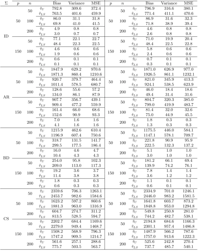
3.1 Finite sample performance of location estimates (ˆτU and ˆτLS) withτ0 = 0.2 (in 10−4) 141 3.2 Finite sample performance of location estimates (ˆτU and ˆτLS) withτ0 = 0.5 (in 10−4) 142 3.3 Coverage probability and average length of seven confidence intervals for the ID covariance model . . . 143

3.4 Coverage probability and average length of seven confidence intervals for the AR covariance model . . . 144

3.5 Coverage probability and average length of seven confidence intervals for the BD covariance model . . . 145

3.6 Coverage probability and average length of seven confidence intervals for the CS covariance model . . . 146

3.7 Coverage probability and average length of seven confidence intervals for different interactions . . . 147

(10)

List of Figures

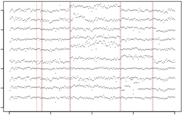
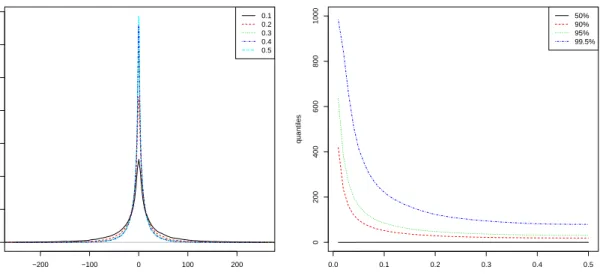
2.1 The time series plot for ACGH data set with the first 10 patients and 200 loci. The black dotted line indicates the change points identified by WBS and the read dotted line represents the change point locations detected by INSPECT . . . 88 3.1 Density plot and quantile plot for different values of τ0 . . . 140

(11)

Chapter 1

Hypothesis Testing for

High-dimensional Time Series

via Self-normalization

1.1 Introduction

In this paper, we study the problem of hypothesis testing for the mean vector of a p-dimensional stationary time series {Yt}Nt=1. Mean testing for independent and identically distributed (i.i.d.

hereafter) data is a classical problem in multivariate analysis. When the dimension p is fixed as the sample size N grows, Hotelling’s T2 test is a classical one and it enjoys certain optimality properties under Gaussian assumptions [see Anderson (2003), Theorem 5.6.6 (pp. 196)]. There is a recent surge of interest in the high-dimensional setting, where p grows as the sample size N → ∞, motivated by the collection of high-dimensional data from many areas such as biological science, finance and economics, and climate science among others. See Bai and Saranadasa (1996), Srivastava and Du (2008) , Srivastava (2009), Chen and Qin (2010), Lopes et al. (2011), Secchi et al. (2013), Cai et al. (2014), Gregory et al. (2015), Xu et al. (2016), Zhang (2017), Pini et al. (2018) and references cited in these papers. All of these works dealt with i.i.d. data, and the methods and theory developed may not be suitable when the high-dimensional data exhibits serial dependence. High-dimensional data with serial or temporal dependence occurs in many fields, such as large-dimensional panel data in economics, fMRI data collected over time in neuroscience, and spatio-temporal data analyzed in climate studies.

The focus of this article is on inference for the mean of a high-dimensional time series. When the dimension is low and fixed, several methods have been developed to perform hypothesis testing for the mean of a multivariate time series with weak dependence, e.g. normal approximation with consistent estimation of the long-run covariance matrix [Andrews (1991)], subsampling [Politis and Romano (1994)], moving block bootstrap [K¨unsch (1989), Liu and Singh (1992)] and variants, block-wise empirical likelihood [Kitamura (1997)] and the self-normalization method [Lobato (2001),Shao

(12)

(2010)]. When the dimension is high and grows with respect to the sample size, little is known about the validity of the above-mentioned methods. It is worth noting that Jentsch and Politis (2015) showed the asymptotic validity of a multivariate version of the linear process bootstrap [McMurray and Politis (2010)] for inference about the mean when the dimension of a time series is allowed to increase with the sample size. However, the growth rate ofphas to be slower than that of the sample size, which rules out the case p > N. Recently, Zhang and Wu (2017) considered the problem of approximating the maxima of sums of high-dimensional stationary time series by Gaussian vectors under the framework of functional dependence measure [Wu (2005)]. Their ap-proach, which can be viewed as an extension of Chernozhukov et al. (2013) from the i.i.d. setting to the stationary time series setting, is applicable to tests about the mean of high-dimensional time series. Another related work along this line is Zhang and Cheng (2018), who obtained sim-ilar Gaussian approximation results as those presented in Zhang and Wu (2017) but under more stringent assumptions. Note that Zhang and Cheng (2018) used a blockwise multiplier bootstrap as an extension of multiplier bootstrap used in Chernozhukov et al. (2013) to accommodate weak serial dependence, whereas Zhang and Wu (2017) adopted direct estimation of the long-run covari-ance matrix, which also requires selecting a block size in its batched mean estimate. Both Zhang and Cheng (2018) and Zhang and Wu (2017) also extended their approaches to inference for other quantities beyond the mean, and their theory allowspto grow at either a polynomial or exponential rate as a function ofN depending on the moment and dependence assumptions.

In this article, we propose to adopt a U-statistic based approach to the testing problem, extending the work of Chen and Qin (2010), who first proposed to use a U-statistic in a high-dimensional two-sample mean testing problem for independent data. Our U-statistic is however different from the one proposed for i.i.d. data in that we remove pairs of observations that are within m time points of each other, where mis a trimming parameter, to alleviate the bias caused by weak serial dependence. Under the framework of high-dimensional nonlinear causal processes, we show that our U-statistic is asymptotically normal under the null hypothesis. The norming sequence is dependent on the Frobenius norm of the long run covariance matrix (i.e., kΓk_F), whose rate of divergence is not assumed to be known. To perform the test, one approach is to find a ratio-consistent estimator

(13)

of kΓk_F, say usingkΓkb _F, so that kΓkb _F kΓkF

→1 in probability, (1.1.1)

where bΓ is the usual lag window estimator. Such an estimator typically involves a bandwidth pa-rameter, and its consistency has been shown in the low and fixed-dimensional context; see Andrews (1991), Newey and West (1987). In the high-dimensional context, Chen and Wu (2019) showed the so-called normalized Frobenious norm consistency, which implies the ratio consistency (1.1.1), in the context of trend testing. However, no discussion about the choice of the bandwidth parameter seems offered in Chen and Wu (2019) and their result is restricted to linear processes.

To circumvent the difficulty, we take an alternative approach, and our test is based on the idea of self-normalization (SN, hereafter). SN for the mean of a time series was first proposed by Lobato (2001); also see Kiefer et al. (2000) for a related development in the time series regression framework around the same time. Later SN was extended by Shao (2010) and coauthors to various inference problems in time series analysis; See Shao and Zhang (2010), Zhou and Shao (2013), Kim et al. (2015) and Zhang et al. (2011) among others. The basic idea of self-normalization in the time series context is that it uses an inconsistent variance estimator as the studentizer, and the resulting studentized test statistic can still be (asymptotically) pivotal and its limiting null distribution and critical values can be approximated by Monte-Carlo simulations. It has the appealing feature of requiring no tuning parameters for some problems or fewer tuning parameters compared to existing inference procedures, but all existing SN-based methods are limited to inference for a parameter with finite and fixed dimension; see Shao (2015) for a recent review. Here we make the first attempt to extend the idea of SN for inference in high-dimensional time series and for a parameter of high/growing dimension. To this end, we study the weak convergence of a recursive version of our full-sample based U-statistic. Under suitable assumptions, we show that the limiting process is a time-changed Brownian motion, which is different from the standard Brownian motion limit in the application of SN for low-dimensional weakly dependent time series. The limiting null distribution of our SN-based test statistic is still pivotal and its critical values are tabulated via simulations.

One appealing feature of our test statistic is its adaptiveness to the unknown order ofkΓk_F, which gets canceled out in the limit of our self-normalized test statistic. This seems to be discovered for

(14)

the first time, as the convergence rate is typically known or needs to be estimated in the use of SN for a low-dimensional parameter; see Shao (2015). On the theory side, we extend the martingale approximation argument to the high-dimensional setting. In our result, the dimension p can grow at an exponential rate as a function ofN under suitable moment and weak dependence assumptions on the processes. Compared to the maximum type tests proposed by Zhang and Wu (2017), Zhang and Cheng (2018), our test is ofL2 type and it targets dense and weak alternatives, whereas theirs

are expected to be more powerful for strong and sparse alternatives. As two important applications, we apply our tests to testing for the bandedness of a covariance matrix and testing for white noise for dimensional time series. Finally, we mention a few recent works on inference for high-dimensional time series. Lam and Yao (2012) proposed a static factor model for high-high-dimensional time series and focused on estimating the number of factors; Basu and Michailidis (2015) investi-gated the theoretical properties ofl1-regularized estimates in the context of high-dimensional time

series and introduced a measure of stability for stationary processes using their spectral properties that provides insight into the effect of dependence on the accuracy of the regularized estimates; Paul and Wang (2016) presented results related to asymptotic behavior of sample covariance and autocovariance matrices of high-dimensional time series using random matrix theory.

The rest of the article is organized as follows. Section 1.2 introduces the basic problem setting and the notations we use throughout the paper. Section 1.3 presents our self-normalized statistic as well as related asymptotic results. Section 1.4 introduces two extensions of the self-normalized statistic to bandedness and white noise testing and Section 3.4 presents all finite sample simulation results. Section 2.6 concludes. Finally all the technical details are included in the Appendix and Supplemental Material.

1.2 Problem Setting

Assume that we have a p-dimensional stationary nonlinear time series

(15)

for some measurable function g, where {_t}∞

t=−∞ are i.i.d. random elements in some measurable space. For the j-th element of Yt, denoted as Yt,j, assume

Yt,j =µj+gj(t, t−1,· · ·),

wheregj is thejth component of the mapg, andµ= (µ1,· · · , µp)T. We assumeE[g(t, t−1,· · ·)] =

0. Later we shall introduce suitable weak dependence assumptions under the above framework, which was initially proposed by Wu (2005), who advocated the use of physical dependence measure in asymptotic theory of time series analysis; see Wu (2011) for a review. Our weak dependence condition is characterized by a variant of the Geometric Moment Contraction [see Hsing and Wu (2004), Wu and Shao (2004), Wu and Min (2005)], which was found very useful for studying nonlinear time series and also verifiable for many linear and nonlinear time series models; see Shao and Wu (2007).

Throughout the paper, we let Σ0 = V ar(Yt) denote the marginal covariance matrix and Γ :=

P∞

k=−∞cov(Yt, Yt+k) denote the long-run covariance matrix ofYt. We defineFt=σ(t, t−1,· · ·, 1,

0, −1,· · ·) as the natural filtration generated by{t}, and defineFt0 =σ(t, t−1,· · · , 1, 00, 0−1,· · ·)

where 0_t is an i.i.d. copy of t which is independent from {t}t∈Z. We use k · kF to denote the

Frobenius norm andk · kto denote the spectral norm for a matrix (vector). We letk · kh be theLh

norm for random vectors. We defineEt(·) :=E(·|Ft) andE0t(·) :=E(·|Ft0). For any random element

Xt=X(Ft) which is a function ofFt, we defineXt0 =X(Ft0). All asymptotic results are under the

regime min(N, p)→ ∞.

Given a stretch of observations Yt, t = 1,· · ·, N, from the above process, we are interested in

testing the hypothesis that

H0 :µ=µ0 v.s. H1:µ6=µ0. (1.2.1)

Without loss of generality, we letµ0 = 0. Ifµ0 6= 0, we can apply our test to{Yt−µ0}Nt=1.

(16)

¯

YN =N−1PNt=1Yt is the sample mean. For example, if we use L2 distance, then

kY¯N−0k22 = 1 N2 N X t=1 N X s=1 Y_tTYs.

However the distribution for the above statistic is not easy to derive, in part because whentands are close to each other, the correlation betweenYtandYsinduces a ‘bias’ term (under the null) that

needs to be eliminated by consistent estimation; see Ayyala et al. (2017). Since the auto-correlation can be viewed as a nuisance component for mean inference, we propose to avoid its direct estimation by removing the cross product between observations that are too close to each other in time. To this end, we consider the test statistic

Tn= n+ 1 2 −1 n X t=1 t X s=1 Y_tT₊_mYs, (1.2.2)

where n = N −m and m < N is a trimming parameter which satisfies 1/m+m/N = o(1) as min(p, N)→ ∞. See Chen and Wu (2019) for a similar trimming idea in testing for the form of the trend of multivariate time series. Letθ=µTµ∈_R1 _{be the scalar parameter of interest. Then}_µ_{= 0}

is equivalent toθ= 0. Hence Tn can be viewed as a one sampleU-statistic for time series; see Lee

(1990). The trimming parameter controls the amount of bias since the bias E(Tn)−θdepends on

m and tr(Σh), h=m, m+ 1,· · ·, where Σh =cov(Yt, Yt+h). The larger values of m correspond to

smaller bias, which is intimately related to the accuracy of size; the smaller values ofmcorrespond to more pairs of observations used in the test, which can lead to more power. Section 1.5.1 offers numerical evidence and some discussion of the role ofm in detail. It is worth noting that another commonly used distance is kY¯Nk∞, which has been studied recently in Zhang and Wu (2017) and

Zhang and Cheng (2018). See Section 1.5.1 for some numerical comparison.

Throughout the paper, we use “→” to denote convergence in probability and “p →” to denoteD convergence in distribution. LetD[0,1] be the space of functions on [0,1] which are right continuous and have left limits, endowed with the Skorokhod topology (Billingsley (2008)). Denote by “ ” weak convergence inD[0,1]. We useA.B to represent thatAis less than or equal tocB for some constantc >0.

(17)

Under suitable moment and weak dependence assumptions on Yt, we can show that (n+ 1)Tn/( √ 2kΓkF) D →N(0,1)

under the null; see Corollary 1.3.8. This motivates us to define the process

Tn(r) := bnrc X t=1 t X s=1 Y_tT₊_mYs, r∈[0,1]

and study its process convergence inD[0,1]. Under the null hypothesis whereµ0 = 0, consider the

decomposition

Yt=Dt−ξt,

whereDt:=P∞_k₌₀[Et(Yt+k)−Et−1(Yt+k)] and ξt:=De_t−De_t₋₁,where De_t:= P∞

k=1Et(Yt+k).

By simple calculation we can show that (Dt,Ft) is a martingale difference sequence. Martingale

approximation for the partial sums of a stationary process has been investigated by Gordin (1969), Hall and Heyde (2014), Wu and Woodroofe (2004), Wu (2007), among others. All these works are done in a low-/fixed-dimensional setting. By contrast, we shall show that it still works for our U-statistic and in the high-dimensional setting. Based on the above decomposition, we write

Tn(r) = bnrc X t=1 t X s=1 Y_tT₊_mYs = bnrc X t=1 t X s=1 (Dt+m−ξt+m)T(Ds−ξs) = bnrc X t=1 t X s=1 DT_t₊_mDs− bnrc X t=1 t X s=1 ξ_tT₊_mDs− bnrc X t=1 t X s=1 D_tT₊_mξs+ bnrc X t=1 t X s=1 ξ_tT₊_mξs =Sn(r)−R1,n(r)−R2,n(r) +R3,n(r), whereSn(r) =Pb_t₌₁nrcPt_s₌₁DtT+mDs,R1,n(r) =Pb_t₌₁nrcPt_s₌₁ξtT+mDs,R2,n(r) =Pb_t₌₁nrcPt_s₌₁DtT+mξs, and R3,n(r) =P bnrc t=1 Pt s=1ξtT+mξs. Note that Tn(r) = 0 if r <1/n.

Remark 1.2.1. It is worth mentioning that a straightforward extension of the SN idea in Lobato (2001) does not really work in the setting p > N. To elaborate the idea, we shall briefly review the SN method in Lobato (2001). Let B(r), r ∈ [0,1] be the standard Brownian motion and

(18)

B_q(r), r∈[0,1] be aq-dimensional vector of independent Brownian motions. Define

Uq=Bq(1)TJq−1Bq(1), whereJq =

Z 1

0

[Bq(r)−rBq(1)][Bq(r)−rBq(1)]Tdr.

The critical values for Uq, q = 1,· · ·,20 have been tabulated by Lobato (2001). For Yt ∈ Rp, let D2_N =N−2PN

t=1{

Pt

j=1(Yj−Y¯N)}{

Pt

j=1(Yj−Y¯N)}T be thep×pnormalization matrix. Ifpis small

and fixed, then under the null and suitable assumptions, we haveN( ¯YN−µ0)T(D_N2)−1( ¯YN−µ0)

D → Up, as N → ∞. The key ingredient is to replace the consistent estimator of Γ, as used in the

traditional approach, with the inconsistent estimator D2_N. Since the normalization factor D_N2 is proportional to Γ, the nuisance parameter Γ is canceled out in the limiting distribution of the resulting statistic. It is not hard to see that the SN approach is not feasible when p > N, since D2_N is not invertible in this case. Even whenp < N, both empirical and theoretical studies suggest that the approximation error grows with the dimension p [Sun (2014)]. So the use of this form of self-normalization can result in a big size distortion whenp is comparable to N.

1.3 Technical Assumptions and Theoretical Results

To facilitate our methodological and theoretical development, we shall introduce some technical assumptions. We first extend the GMC (Geometric Moment Contraction) condition in Hsing and Wu (2004) and Wu and Shao (2004) to the high-dimensional setting.

Definition 1.3.1. Let {Y_t}_t∈_Z be ap×dmatrix-valued stationary process withYt=h(Ft)for some

h. It has the Uniform Geometric Moment Contraction (UGMC(k)) property if there exists some positive number k such that

sup i=1,···,p,j=1,···,d E[|Y0,i,j|k]< C <∞ and sup i=1,···,p,j=1,···,dE

(|Yt,i,j−Yt,i,j0 |k)≤Cρt, t≥1

for some 0 < ρ < 1 and a positive constant C that do not depend on p or d. For vector-valued stationary process, the same definition can be applied by letting d= 1.

(19)

Remark 1.3.2. DefineF_t,_{_k_} =σ(t, ..., k+1, 0k, k−1, ...), and it is easy to see thatFt0 =Ft,{0,−1,...}.

Let Yt,{k} = g(Ft,{k}). In Zhang and Wu (2017) and Zhang and Cheng (2018), they defined the

functional dependence measure for each component process as

θt,q,j =kYt,j−Yt,j,{0}kq=kYt,j−gj(Ft,{0})kq,

and let Θm,q,j = P∞_t₌_mθt,q,j. Throughout these two papers, they imposed conditions on Θm,q,j.

Specifically, Zhang and Cheng (2018) considered a special case where maxjΘm,q,j ≤ Cρm with

ρ∈(0,1) and some constant C. Under this condition,

kY_t,j −Y_t,j0 k_q =kY_t,j−Yt,j,{0}+Yt,j,{0}−Yt,j,{0,−1}+Yt,j,{0,−1}−Yt,j,{0,−1,−2}+· · · kq ≤kYt,j −Yt,j,{0}kq+ ∞ X l=0 kY_t,j,{0,...,−l}−Yt,j,{0,...,−l,−(l+1)}kq ≤Cρt ∞ X l=0 ρl ! ≤ C 1−ρ ρt, and maxjkYt,j−Yt,j0 kq ≤ C 1−ρ

ρt, which is just the definition of UGMC(q) defined above. Con-versely, if we assume UGMC(q), then

kYt,j−Yt,j,{0}kq≤ kYt,j−Yt,j0 kq+kYt,j0 −Yt,j,{0}kq=kYt,j−Yt,j0 kq+kYt+1,j−Yt0+1,jkq

≤Cρt+Cρt+1=C(1 +ρ)ρt,

which means maxjΘm,q,j ≤ C(1 +ρ)ρm. Hence our UGMC assumption is equivalent to that in

Zhang and Cheng (2018).

In Zhang and Wu (2017), they defined a so-called “dependence adjusted norm” by letting

kY.jkq,α= sup m≥0

(m+ 1)αΘm,q,j

which is equivalent to the classical Lq norm for i.i.d. data. Further they defined

Ψq,α= max 1≤j≤qkY.jkq,α and Υq,α=   p X j=1 kY.jkqq,α   1/q ,

(20)

gen-eral weaker than ours in the sense that no (uniform) moment assumptions are required for each component series and also algebraic decay of Θm,q,j for each j is allowed.

Assumption 1.3.3. Assume that{Y_t}_t∈_Z are Rp-valued stationary time series withE(Yt) = 0 and

they satisfy A.1 sup₁≤j≤p P∞ k=0kE0[Yk,j]k8 < C. A.2 {Y_t} is UGMC(8). A.3 P∞ h=0kΣhk=o(kΓkF). A.4 p4ρm=o(kΓk4 F) and 1/m+m/N =o(1). A.5 For h= 2,3,4, Pp j1,···,jh=1|cum(Dt1,j1,· · ·, Dtl,jl,Detl+1,jl+1,· · · ,Deth,jh)|=O(kΓk h F), for any l= 0,· · · , h. A.6 Pp j1,···,j4=1|cov(∆t1,j1,j2,∆t2,j3,j4)|=O(kΓk 4

F)for anyt1, t2, where∆t=E(Dt+1DTt+1|Ft)and

∆t,i,j is the (i, j)th element of ∆t.

Throughout the paper, we use cum(A1,· · · , Ad) to denote the joint cumulant of drandom

vari-ables A1,· · · , Ad; see page 19 of Brillinger (2001) for a formal definition of the dth order joint

cumulant.

Remark 1.3.4. Assumption A.1 indicates that sup_jkY₀_,jk₈, sup_jkD₀_,jk₈ and sup_jkDe₀_,jk₈ are all bounded. To see this,E0[Y0,j] =Y0,j and kD0,jk8≤ kY0,jk8+kDe₀_,jk₈+kD−e ₁_,jk₈. Moreover,

kDe₀_,jk₈≤ ∞ X

k=1

kE0[Yk,j]k8 < C.

Assumption A.1 can be shown to be implied by Assumption A.2 but since Assumption A.1 was used explicitly at several places, we put it up for the ease of reference. Assumption A.2 can be verified for stationary ARMA processes. The geometric decay rate associated with UGMC condition can actually be relaxed to a polynomial rate, but at the expense of more complicated details. Assumption A.3 effectively restricts the growth rate of P∞

h=0kΣhk relative tokΓkF, which can be

(21)

the trimming parameterm, and it implies that the bias after trimming is asymptotically negligible. Assumption (b) can be verified under some mild conditions. See Section 1.3.2 for the verification for linear process. Furthermore, we have the following result.

Proposition 1.3.5. Assumption (b) can be satisfied if either one of the following is true: 1.

|cum(D_t₁_,j₁,· · · , Dtl,jl,Detl+1,jl+1,· · ·,Deth,jh)| ≤Cρ

maxkjk−minkjk _(1.3.1) for any t1≤ · · · ≤th,l= 0,· · ·, h, and that all diagonal elements of Γare greater than some

positive constant c0.

2. The conditional expectations of component processes areq-dependent, i.e.,Et0(gi(t1, t1−1,· · ·))

is independent of Es0(gj(s1, s1−1,· · ·)) for any t1 ≥t0, s1 ≥s0, and |i−j| ≥ q, where q is

a positive fixed integer which is independent ofn and p.

Theorem 1.3.6. Under Assumptions 1.3.3, we have

√ 2

nkΓk_FSn(r) B(r

2₎ _in _D[0,_1].

Theorem 1.3.7. Under Assumptions 1.3.3, we have

max r∈[0,1] √ 2 nkΓk_FRi,n(r) p →0 for i= 1,2,3.

Theorems 1.3.6 and 1.3.7 suggest that the leading termSn(r) dominates inTn(r) and that the

re-mainder termsRi,n(r), i= 1,2,3 are asymptotically negligible. Thus the martingale approximation

still works in our high-dimensional setting and for our U-statistic. Corollary 1.3.8. Under Assumption 1.3.3, we have

√

2

nkΓkFTn(r) B(r

2₎ _in _D[0,_1].

We introduce our self-normalizer as

W_n2= 1 n n X k=1 Tn(k/n)− k(k+ 1) n(n+ 1)Tn(1) 2 . (1.3.2)

(22)

Then we define our self-normalized test statistic TSN,n as TSN,n := Tn(1)2 W2 n . (1.3.3)

Theorem 1.3.9. Under H₀ and Assumptions 1.3.3, we have

TSN,n D → K:= B(1) 2 R1 0(B(u2)−u2B(1))2du . (1.3.4)

Compared to the use of self-normalization in the low-dimensional setting [Lobato (2001), Shao (2010)], there are some interesting differences we want to highlight. Firstly, due to the use of U-statistics, the limit of the process Tn(r) (after some standardization) is a time-changed Brownian

motion and it differs from the Bronwian motion limit for the partial sum process in Lobato (2001) and Shao (2010). Secondly, the null limit of the self-normalized test statistic K differs from that used in the low-dimensional case. Since it is still pivotal, we can obtain the simulated quantiles for K, as presented in the table below. Thirdly, we had to introduce a trimming parameter m to eliminate the need to estimate autocovariances, which is not needed in the low-dimensional case. Such trimming serves as a bias reduction tool, and it seems necessary to preserve the main feature of self-normalization.

To approximate the theoretical quantiles of K, (Kα denotes the α quantile of K), we use a

sequence of i.i.d. standard normal random variables with length 106to approximate one realization of the standard Brownian motion path. We construct 106 Monte-Carlo replicates for this path and then the empirical quantiles for K are summarized in the following table.

α 0.8 0.9 0.95 0.99 0.995

K_α 18.19 34.15 54.70 118.49 153.94

Table 1.1: Upper quantiles of the distributionK simulated based on 106 Monte Carlo replications

Remark 1.3.10. Chen and Qin (2010) first proposed to use a U-statistic in a high-dimensional two sample mean testing problem for independent data and they used normal approximation and a direct ratio-consistent variance estimate; see page 814 for the expression of the variance estimate and their Theorem 2 for the ratio-consistency statement. In comparison, our U-statistic is different

(23)

from theirs in that (1) we are using a one sample U-statistic; (2) we have to introduce a trimming parameter m to remove pairs of observations that are within m lags to avoid direct estimation of the bias caused by the temporal correlation. Our U-statistic is tailored for weakly dependent time series, see Lee (1990); (3) the nuisance parameter associated with our test statistic is kΓkF,

for which a ratio-consistent estimator still involves a bandwidth parameter (see Chen and Wu (2019)), whereas the nuisance parameter for the statistic in Chen and Qin (2010) is kΣkF which

can be consistently estimated without any tuning parameter. Our self-normalizer is not a consistent estimator of but proportional tokΓk_F, and the resulting self-normalized test statistic has a pivotal limit under the null.

Another appealing and distinctive feature of the SN-based test in the high-dimensional setting is that the use of self-normalization in the low-dimensional context requires the knowledge of the convergence rate to a certain stochastic process, say standard Brownian motion. However in the high-dimensional setting we present here, we do not know the exact diverging rate of kΓkF, but

within the self-normalization procedure, this nuisance parameter can be canceled out from both the numerator and the denominator. In other words, the applicability of the SN method is considerably broadened.

1.3.1 Limit Theory under a Local Alternative

Under the alternative,E[Yt] =µ6= 0. ThenTn(r) can be decomposed as

Tn(r) = bnrc X t=1 t X s=1 Y_tT₊_mYs= bnrc X t=1 t X s=1 (Yt+m−µ+µ)T(Ys−µ+µ) = bnrc X t=1 t X s=1 (Yt+m−µ)T(Ys−µ) + bnrc+ 1 2 kµk2₂ + bnrc X t=1 t(Yt+m−µ)Tµ+ bnrc X s=1 (bnrc −s+ 1)(Ys−µ)Tµ.

Theorem 1.3.11. Under Assumptions 1.3.3 and the alternative hypothesisE[Yt] =µ6= 0, we have

1. If kµk=o(n−1/2kΓk1_F/2), then TSN,n D → B(1) 2 R1 (B(u2₎₋_u2_B(1))2_du

(24)

and P(TSN,n ≥ Kα)→α. Thus the SN-based test has trivial power asymptotically. 2. If √nkµkkΓk−_F1/2 →c, where c∈(0,∞), then TSN,n D → (B(1) +c 2_/√₂₎2 R1 0(B(u2)−u2B(1))2du

and P(TSN,n ≥ Kα)→β ∈(α,1). Thus our test has nontrivial power asymptotically.

3. If √nkµkkΓk−_F1/2 → ∞, then TSN,n p

→ ∞ andP(TSN,n≥ Kα)→1. Thus the limiting power

is 1.

Remark 1.3.12. Theorem 1.3.11 suggests that the local neighborhood around the null for which there is a nontrivial power is characterized bykµk=cn−1/2kΓk1_F/2. In the special case when Γ =Ip,

µ=δ(1,· · ·,1)T where δ=Cn−1/2p−1/4, for someC 6= 0, existing methods which are designed to test against sparse alternatives fail to detect such dense and faint alternatives; see Cai et al. (2014). By contrast, TSN,n is able to achieve nontrivial power.

1.3.2 Linear Processes

A direct application of the main theorem is to the case of linear processes. Consider the data generating process Yt=µ+ ∞ X k=0 ckt−k, (1.3.5)

where t are i.i.d. p-dimensional innovations with mean 0 and ck are p×p coefficient matrices.

Applying the martingale approximation, we can obtain by simple calculation that Dt = C(1)t

whereC(1) =P∞ k=0ck and e Dt= ∞ X j=0   ∞ X k=j+1 ck  t−j.

This is exactly the well-known Beveridge Nelson (BN) decomposition described in Phillips and Solo (1992). In this case, the long-run covariance matrix is Γ =C(1)ΣC(1)T, where Σ=V ar(0).

Assumption 1.3.13. Assume that {Yt} is generated from (1.3.5) with µ= 0 and that

B.1 sup₁≤j≤pkt,jk8 < C. B.2 P∞

(25)

B.3 P∞ h=0kΣhk=o(kΓkF). B.4 p4_ρm₌_o(kΓk4 F) and 1/m+m/N =o(1). B.5 For h= 2,3,4, Pp j1,···,jh=1|cum(Dt1,j1,· · ·, Dtl,jl,Detl+1,jl+1,· · · ,Deth,jh)|=O(kΓk h F), for any l= 0,· · · , h.

Corollary 1.3.14. Under Assumptions 1.3.13, we have

√ 2

nkΓk_FTn(r) B(r

2₎ _in _D[0,_1].

The assumptions B.3 and B.5 can be verified for many weakly dependent time series models. In the following proposition, we shall present some more primitive assumptions for the vector AR(1) model, i.e., Yt =AYt−1+t, for t∈Z. For simplicity, we assume A to be symmetric and t to be

i.i.d. p-dimensional random vectors with mean zero and covariance matrix Σ.

Proposition 1.3.15. Assume thatYt are generated from a V AR(1) model satisfying

1. |Γi,i|> c0 >0 for some positive constant c0 and all i= 1,· · · , p; 2. kΣk=o(kΓkF),

3. lim sup_p_→∞kAk< c1<1 for some positive constant c1.

Then B.3 can be verified. Furthermore, if we substitute condition 3 with

4. lim sup_p→∞kAk1 < c1 <1 for some positive constant c1, and in addition assume

5. Pp

k1,···,kh=1|cum(0,k1,· · · , 0,kh)|=O(kΓk

h

F), for h= 2,3,4,

then B.5 holds.

Remark 1.3.16. Under the conditions in Proposition 1.3.15, it is easy to see that the order of kΓkF is between

√

p and p. When kΓkF is of order p, theoretically we do not have any explicit

restriction on the growth rate ofp as a function of n(orN). In this case, the condition B.4 holds as long as the trimming parameter mgrows to infinity but slower than N. WhenkΓkF is of order

(26)

√

p, we can allow the order ofpto beenβ, for anyβ ∈(0,1), by choosingmto be of ordernγ, where γ ∈(β,1). Condition 5 in Proposition 1.3.15 basically restricts the coordinate dependence of the innovation sequencet. If the components oft satisfy certainm-dependence or geometric moment

contraction condition [see Wu and Shao (2004)], thenPp

k1,···,kh=1|cum(0,k1,· · · , 0,kh)|=O(p), so

condition 5 is satisfied.

1.4 Applications

The SN-based test can be extended to test the bandedness of the covariance matrix of high-dimensional time series (HDTS). Assume that we have a stationary s-dimensional time series (Xt)t∈Z with E(Xt) = 0 for notational simplicity (we can apply our method to demeaned data in

practice). For high-dimensional temporally-independent data, the covariance matrix Σ =Cov(Xt,

Xt) = (γjk)j,k=1,···,s is an important measure of the dependence among components of Xt, and

for time series, it measures the contemporaneous component-wise dependence. In this section, we slightly abuse the notation and use Σ to denote the covariance matrix of Xt, Σh to denote the

autocovariance matrix of Xt at lag h. Qiu and Chen (2012) first developed a test for bandedness

of Σ, motivated by promising results regarding banding and tapering the sample covariance in estimating Σ; see Bickel and Levina (2008), Cai et al. (2010) among others. Specifically, for a given bandwidth L, they test

HL,0 : Σ =BL(Σ), versusHL,1: Σ6=BL(Σ)

where BL(Σ) = (γjkI{|j−k| ≤ L})s×s is a banded version of Σ with bandwidth L. Note that

diagonal matrices are the simplest among banded matrices, and testing for Σ being diagonal (or the so-called sphericity hypothesis in classical multivariate analysis) in the high-dimensional setting has been considered in Ledoit and Wolf (2002), Jiang (2004), Schott (2005), Chen et al. (2010) and Cai and Jiang (2011), among others. All of the above works are for independent data, and they seem no longer applicable to HDTS due to temporal dependence. As a practical motivation, we note that in the analysis of fMRI functional connectivity for brain networks in the format of multivariate time series, Σ has been used to characterize functional connectivity; see Hutchison et al. (2013). As

(27)

pointed out by a referee, Liu et al. (2018) studied the sphericity hypothesis testing in the context of high-dimensional time series. However, their test statistic seems infeasible as they assumed certain unknown quantities in their test to be known and did not offer any consistent estimates for these unknown quantities.

To testHL,0, we letXt= (Xt1,· · ·, Xts)T andγjk =Cov(Xtj, Xtk) forj, k= 1,· · ·, s. Further let

I ={(j, k) :|j−k|> L, j > k}. Then the null hypothesisHL,0is equivalent to 0 =γ = (γjk)(j,k)∈I ∈ RPL_{, where}_P

L= (s−L)(s−L−1)/2. LetZt,jk =XtjXtk, and Yt= (Zt,jk)(j,k)∈I ∈RPL×1_{. Then}

we can formulate this as a testing-many-means problem based on the transformed observations (Yt)Nt=1.

In addition, we can also apply the SN-based test to testing the white noise hypothesis for HDTS. Testing for white noise is an important problem in time series analysis and it is indispensable in diagnostic checking for linear time series modeling. There is a huge literature for univariate and low-dimensional vector time series; see Li (2004) for a review of the literature of univari-ate time series and Hosking (1980), Li and McLeod (1981) and L¨utkepohl (2005), among others for the diagnostic checking methods for vector time series. The literature on white noise test-ing for high-dimensional time series is quite recent. Chang et al. (2017) proposed to use max-imum of absolute autocorrelations and cross correlations of component series as a test statis-tic and its null distribution is approximated by Gaussian approximation [Chernozhukov et al. (2013)]. Li et al. (2018) used the sum of squares of the eigenvalues in the symmetrized sam-ple autocovariance matrix at a certain lag, and the limiting null distribution is derived using tools from random matrix theory. Specifically, they both test H0,d : Σ1 = Σ2 = · · · = Σd =

0, where d is a fixed and pre-specified lag and Σh = Cov(Xt, Xt−h) = (γh,jk)j,k=1,···,s, where

γh,jk = Cov(Xtj, X(t−h)k) = E(Zt,h,jk) and Zt,h,jk = XtjX(t−h)k. Let Yt,h = (Zt,h,jk)j,k=1,···,p =

(Zt,h,11, Zt,h,12,· · · , Zt,h,1s, Zt,h,21, Zt,h,22,· · · , Zt,h,2s,· · · , Zt,h,s1, Zt,h,s2,· · ·, Zt,ss)T, which is ans2×

1 vector. Then Σh = 0 is equivalent to E(Yt,h) = 0, and H0,d can be tested using our SN-based

(28)

1.5 Simulation Results

In this section, we investigate the finite sample performance of SN-based methods for mean testing, bandedness testing of covariance matrices, and white noise testing in subsections 1.5.1, 1.5.2 and 1.5.3, respectively.

1.5.1 Mean Inference

In this subsection, we study the finite sample performance of the proposed method for mean infer-ence. Consider the data generating process

Yt−µ=A(Yt−1−µ) +t,

which is ap-dimensional VAR(1) model. Hereµ=E[Yt] and the innovation sequence{t}are i.i.d.

according to a multivariate normal distribution with mean 0 and covariance Σ where Σ1/2 is a

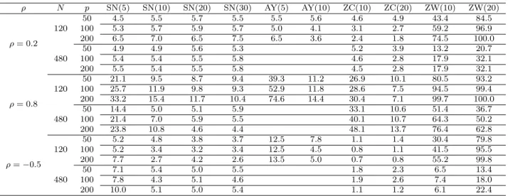
tri-diagonal matrix with diagonal elements all equal to 1, and the first off-diagonal entries all equal to 0.5. We consider two sample sizes,N ∈ {120,480}and three dimensions, p∈ {50,100,200}. For the coefficient matrix A, we simply letA=ρIp and pick ρ∈ {0.2,0.8,−0.5}.

Under the null hypothesis, µ is simply a vector of zeroes. We let µ = 0.8×(1/√p,1/√p,· · ·, 1/√p)T under the alternative. We include four methods and ten statistics in the simulation: (1) Self-Normalized Statistic (m= 5,10,20,30) (Denoted as “SN(5)”, “SN(10)”, “SN(20)”, “SN(30)”); (2) the test proposed in Ayyala et al. (2017). Note that their test assumed the q-dependence for the data generating process but in practice we typically do not know the value of q. We shall set q = 5 and 10 here so the test is denoted as “AY(5)” and “AY(10)”, respectively; (3) the approach proposed in Zhang and Cheng (2018) with the block size used in the block bootstrapbZC ={10,20},

denoted as “ZC(10)” and “ZC(20)”; (4) the approach proposed in Zhang and Wu (2017) with the block size used in batched mean estimate bZW = {10,20}, denoted as “ZW(10)” and “ZW(20)”.

Note that there seems no data driven formula for the block size used in Zhang and Cheng (2018) and Zhang and Wu (2017), and it is indeed an open problem on how to select the optimal block size in the high-dimensional setting. For the choice of our trimming parameter m, we shall let m= 5,10,20,30 and leave the detailed discussion on its role later.

(29)

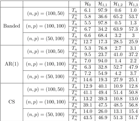
We set the nominal level as 5% and perform 1000 Monte Carlo simulations for N = 120 and N = 480. The computation for the test in Ayyala et al. (2017) is very expensive so only the result for the case N = 120 is shown here. The results are summarized in Tables 1.2 and 1.3. Under the null hypothesis, SN has an accurate size mostly when the dependence is weak (i.e., ρ = 0.2). When the dependence gets stronger (i.e., ρ = 0.8), there are some fairly large size distortion corresponding to m = 5, which is likely due to the bias incurred by using a small m, and the size corresponding to larger m (i.e., m = 20,30) appears much better. When ρ = −0.5, there are slight conservativeness in the size of SN test, but most are quite close to nominal level, especially when m= 10,20,30 and N = 480. By contrast, ZC and ZW showed much more severe size distortion, especially in the (relatively) strong dependent case (i.e., ρ = 0.8). For both block sizes 10 and 20, ZW method appears to fail to provide a reasonable size in almost all cases, whereas ZC method seems to perform better when the block size is 20, although the size appears too liberal when ρ= 0.8 and too conservative whenρ= 0.2 and −0.5. Also we can observe the sensitivity of both ZW and ZC with respect to the block size, the choice of which seems to be an open problem in the high-dimensional setting. The test AY(5) exhibits huge size distortion when ρ= 0.8, which is presumably due to the fact that q = 5 is too small, whereas AY(10) shows much improvements although it is still quite oversized. In the case ρ = 0.2, there are some noticeable size distortions with AY(5) and again AY(10) exhibits more accurate size. Overall the size of SN-based test seems much more satisfactory and stable than ZC and ZW, and outperforms that of AY slightly.

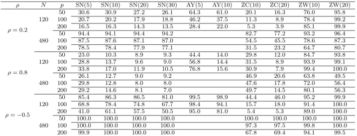
As seen from Table 1.3, which presents the power, SN-based test exhibits highest power when ρ=−0.5, and the power in the caseρ= 0.8 is quite low. This can be explained by the fact that in the limit the power is a monotonic increasing function of √nkµkkΓk−_F1/2, which takes the largest value when ρ = −0.5 and admits the smallest value when ρ = 0.8. The powers for ZW and ZC are a bit hard to interpret due to the strong over-rejection under the null hypothesis. One can present size-adjusted power, but given the severely distorted size we decide not to pursue this. The tests by Ayyala et al. (2017) exhibit higher power than SN-based tests in almost all cases and the power gain appears quite moderate in some cases. This might suggest that if we can completely remove the bias caused by weak temporal dependence and choose the tuning parameter properly, the normal approximation can work reasonably well, outperforming the SN-based test in power. This is consistent with the “better size but less power” phenomenon observed for SN-based test

(30)

as compared to normal approximation in the low-dimensional setting; see Shao (2010). It is also worth noting that for our SN-based test the powers corresponding to m= 20,30 are a little lower than that form = 10 in most cases, and the power for m= 30 is comparable or slightly less than that for m = 20. As we increase m, we expect less power as there are fewer pairs of observations used in the test.

Discussion on the role of m: The trimming parameter m plays an important role in balancing the tradeoff between size distortion and power loss. If m is too small, then the bias might not be negligible especially in the strongly dependent case and this could lead to a big size distortion. If m is too large, then the effective sample size, which is proportional to N −m, is less than the optimal level, which could result in power loss. In general, it would be desirable to come up with a data-driven formula for m that is adaptive to the magnitude of serial dependence, which may require a theoretical characterization of the leading term for the bias and the asymptotic power function. An empirical way of choosing m is to visualize the auto and cross correlations of the time series at hand, and choose a m such that majority of auto and cross-correlations are smaller than some threshold for lags beyond m. Our simulation experience suggests that the size and power performance are relatively stable over a certain range [m0, m1], which might suggest that the

optimal choice ofmis not that critical, as long as we choose a mthat is in the suitable interval. A careful study of this issue is beyond the scope of this paper and is left for future investigation.

ρ N p SN(5) SN(10) SN(20) SN(30) AY(5) AY(10) ZC(10) ZC(20) ZW(10) ZW(20) ρ= 0.2 120 50 4.5 5.5 5.7 5.5 5.5 5.6 4.6 4.9 43.4 84.5 100 5.3 5.7 5.9 5.7 5.0 4.1 3.1 2.7 59.2 96.9 200 6.5 7.0 6.5 7.5 6.5 3.6 2.4 1.8 74.5 100.0 480 50 4.9 4.9 5.6 5.3 5.2 3.9 13.2 20.7 100 5.4 5.4 5.5 5.8 4.6 2.8 17.9 32.1 200 5.5 5.4 5.5 5.8 4.5 2.8 17.9 32.1 ρ= 0.8 120 50 21.1 9.5 8.7 9.4 39.3 11.2 26.9 10.1 80.5 93.2 100 25.7 11.9 9.8 9.3 52.9 11.8 28.6 7.5 94.5 99.4 200 33.2 15.4 11.7 10.4 74.6 14.4 30.4 7.1 99.7 100.0 480 50 14.4 5.0 5.1 5.9 33.1 10.6 51.4 36.7 100 21.4 7.0 5.9 5.5 40.1 10.7 64.3 50.2 200 23.8 10.8 4.6 4.4 48.1 13.7 76.4 62.8 ρ=−0.5 120 50 5.2 4.8 3.8 3.7 12.5 7.8 1.1 1.4 30.4 79.8 100 5.2 3.4 3.2 3.4 12.5 4.5 0.8 1.1 41.5 95.5 200 7.7 2.7 4.2 2.6 13.5 5.0 0.7 0.8 55.2 99.8 480 50 7.1 5.4 5.0 5.5 1.8 2.3 6.5 13.4 100 7.8 4.3 5.1 4.6 1.9 2.6 7.4 18.0 200 10.0 5.1 5.0 5.4 1.1 1.2 6.1 22.4

(31)

ρ N p SN(5) SN(10) SN(20) SN(30) AY(5) AY(10) ZC(10) ZC(20) ZW(10) ZW(20) ρ= 0.2 120 50 30.6 30.9 27.2 26.1 64.3 61.0 20.1 16.3 76.0 95.8 100 20.7 20.2 17.9 18.8 46.2 37.5 11.3 8.9 78.4 99.2 200 16.5 16.3 14.3 13.5 28.4 22.0 5.3 3.9 85.1 99.9 480 50 94.4 94.1 94.4 94.2 82.7 77.2 93.2 96.4 100 87.5 87.6 87.1 87.0 54.5 45.5 78.6 87.3 200 78.5 78.4 77.9 77.1 31.5 23.2 64.7 80.7 ρ= 0.8 120 50 23.0 10.3 8.9 9.3 44.4 14.0 29.8 12.0 84.7 93.8 100 28.8 13.7 9.6 9.0 56.8 14.4 31.5 8.9 93.9 99.1 200 33.8 17.0 11.9 10.5 76.8 15.6 30.9 7.9 99.4 100.0 480 50 26.1 12.7 9.0 9.2 46.9 20.6 63.8 49.5 100 29.8 12.8 8.0 8.0 47.6 17.8 72.0 56.4 200 29.2 14.6 8.1 7.0 49.7 14.5 80.1 56.3 ρ=−0.5 120 50 85.4 86.3 86.5 81.0 99.5 98.9 44.4 46.0 95.2 99.9 100 68.8 78.4 74.8 67.7 98.4 94.1 15.7 18.0 91.4 100.0 200 41.0 61.1 57.5 50.5 95.0 81.0 5.4 5.3 89.0 100.0 480 50 100.0 100.0 100.0 100.0 100.0 100.0 100.0 100.0 100 100.0 100.0 100.0 100.0 97.3 97.5 99.8 100.0 200 99.9 100.0 100.0 100.0 67.8 69.4 94.1 99.5

Table 1.3: Empirical Rejection Rate (in percentage) for the mean testing (H1)

1.5.2 Testing the Bandedness of Covariance Matrix

In this subsection we shall present the simulation result for testing the bandedness of a covari-ance matrix. We modify the model assumptions in Qiu and Chen (2012) by allowing temporal dependence. In particular, we generatep-dimensional Xtfrom the model

Xt,i= k0 X

l=0

γlZt,i−l+δXt−1,i,

where k0 is the bandwidth of the covariance matrix, γ0 = 1 for all cases and other coefficients γl

will be specified later on. We let δ ∈ {0,0.4} and sample Zt,i independently from N(0,1). Notice

that when δ = 0, the observations Xt are i.i.d. We choose the sample size N ∈ {20,50,100} and

the dimension p∈ {20,60}.

We calculate the statistic proposed in Qiu and Chen (2012), denoted as TQC and compare with

our test statistic, denoted asTSN. Note that TQC requires Xt0sto be i.i.d. whereas TSN does not,

thus when δ 6= 0, we should expect an impact on the size of TQC. There is no tuning for TQC

and for TSN we set the trimming parameterm= 10. Under the null hypothesis, we consider three

cases for the bandwidth k0 ∈ {0,2,5}. For k0 = 2, we let γ1 = 0.5, γ2 = 0.25, and for k0 = 5, we

let γ1 =· · ·=γ5 = 0.4. To examine the power, we let k0 = 2,5 and test the null hypothesis that

Σ = Bk0−2(Σ). Those coefficients are the same as those with the same k0 in evaluating the size. We set the nominal level as 5% and run the experiment for 1000 times and record the empirical

(32)

rejection rate.

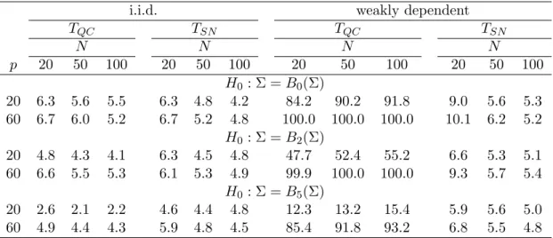
The results under the null are summarized in Table 1.4. For the i.i.d. case, both methods provide reasonably accurate empirical sizes. It is worth noting that the TQC under-rejects the null when

both N and p are small for H0 : Σ = B5(Σ). When data are weakly dependent, we observe that

TQC fails for all cases with a huge size distortion. This is somewhat expected asTQC strongly relies

on the i.i.d. assumption. In comparison,TSN still delivers very good size in most cases, except for

some size distortion when the sample sizeN is too small, i.e.,N = 20.

Table 1.5 shows the power under the alternative. For i.i.d. caseTQC has higher power thanTSN

for all cases. The power gain of TQC over TSN seems to diminish as sample size increases from

N = 20 to N = 100. For weakly dependent data, althoughTQC has a very high empirical rejection

rate in most cases, it should not be taken too seriously because of the huge size distortion under the null. Further, it is noted that the power forTSN is only slightly lower than the i.i.d. case which

indicates TSN still works under the weakly dependent case. In summary, TSN provides a robust

alternative to TQC, which is specifically designed for the i.i.d. data.

i.i.d. weakly dependent

TQC TSN TQC TSN N N N N p 20 50 100 20 50 100 20 50 100 20 50 100 H0: Σ =B0(Σ) 20 6.3 5.6 5.5 6.3 4.8 4.2 84.2 90.2 91.8 9.0 5.6 5.3 60 6.7 6.0 5.2 6.7 5.2 4.8 100.0 100.0 100.0 10.1 6.2 5.2 H0: Σ =B2(Σ) 20 4.8 4.3 4.1 6.3 4.5 4.8 47.7 52.4 55.2 6.6 5.3 5.1 60 6.6 5.5 5.3 6.1 5.3 4.9 99.9 100.0 100.0 9.3 5.7 5.4 H0: Σ =B5(Σ) 20 2.6 2.1 2.2 4.6 4.4 4.8 12.3 13.2 15.4 5.9 5.6 5.0 60 4.9 4.4 4.3 5.9 4.8 4.5 85.4 91.8 93.2 6.8 5.5 4.8

Table 1.4: Empirical Rejection Rate (in percentage) for Testing the Bandedness (under null)

1.5.3 Testing for White Noise

In this subsection we investigate the finite sample properties of our test for white noise. For the trimming parameter we fixm= 10. The nominal level is set as 5%, and we take N ∈ {75,150,300} and p∈ {50,100}. For each experiment we have 1000 Monte-Carlo replicates.We compare our test

(33)

i.i.d. weakly dependent TQC TSN TQC TSN N N N N p 20 50 100 20 50 100 20 50 100 20 50 100 H0 : Σ =B0(Σ) when Σ =B2(Σ) 20 97.7 100.0 100.0 24.0 97.4 100.0 100.0 100.0 100.0 18.6 92.6 99.9 60 98.8 100.0 100.0 26.7 99.3 100.0 100.0 100.0 100.0 20.4 96.1 100.0 H0 : Σ =B3(Σ) when Σ =B5(Σ) 20 19.7 76.3 99.9 6.0 43.1 88.7 52.0 94.1 100.0 6.7 30.0 76.0 60 29.2 84.5 100.0 5.7 40.9 93.2 98.7 100.0 100.0 6.4 26.6 76.5 Table 1.5: Empirical Rejection Rate (in percentage) for Testing the Bandedness (under

alternative)

statistic TSN with the test statisticTC developed in Chang et al. (2017) (with time series PCA),

which targets the sparse alternative and has been implemented in the R package “HDtest”. To examine the size, we generate the data from the model t = Azt, which is the same as the

setting considered in Chang et al. (2017), where A is p×p and zt are p-dimensional i.i.d. from

N(0, Ip). For different loadings,

M1: LetS= (skl)1≤k,l≤p forskl= 0.995|k−l| and then let A=S1/2,

M2: LetA= (akl)1≤k,l≤p with the akl being independently generated from U(−1,1).

To evaluate the power, we letk0 = 12 and generate the data from the model

M₃: t = At−1 +et where {et}t≥1 are i.i.d. p-dimensional random vectors with independent

components from t8 distribution. For the coefficient matrix A, we let Ai,j from U(−0.25,0.25)

independently for any 1≤i, j≤k0 and Ai,j = 0 otherwise.

M4: t = Azt, where zt = (zt,1,· · ·, zt,p)T. For 1 ≤ k ≤ k0, z1,k,· · ·, zN,k are N(0,Σ), where

Σ is N×N matrix with 1 as the main diagonal elements, 0.5|i−j|−0.6 _{as the (i, j)-th element for}

1≤ |i−j| ≤7, and 0 for other elements. Fork > k0,z1,k,· · · , zN,kare independent standard normal

random variables. The coefficient matrixAis generated as follows: ak,l ∼U(−1,1) with probability

(34)

M₅: t = At−1 +et where {et}t≥1 are i.i.d. p-dimensional random vectors with independent

components fromt8 distribution. For the coefficient matrix A, we let Ai,j = 0.9|i−j| for an AR(1)

type structure, then we normalizeA so that kAk= 0.9.

Note that the models M1− M4 were used in Chang et al. (2017) whereas M5 is added to

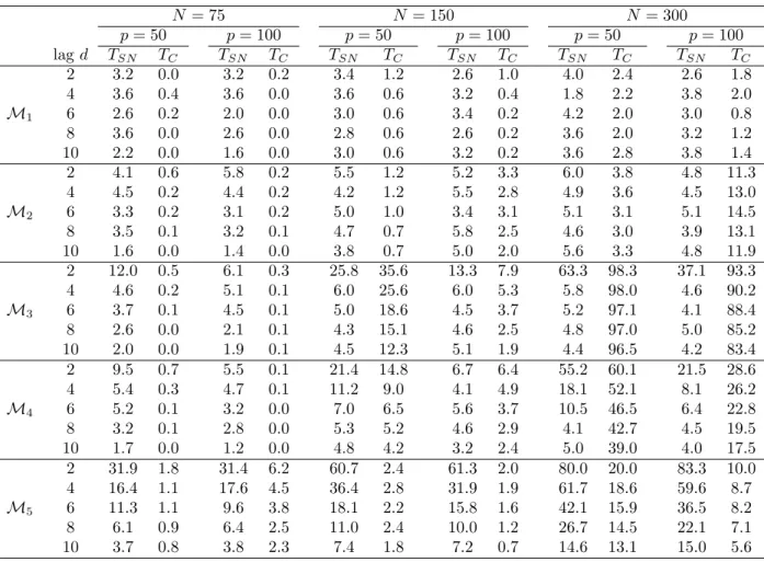
ex-amine the behavior of our test in the case of dense alternative. Results are summarized in Table 1.6. Under the null hypothesis (M₁ & M₂), TSN has an accurate and stable empirical rejection

rate, comparing to the designed nominal level 5%. TC tends to under-reject the null a lot, especially

when N is small. We notice that the empirical rejection rate of TC is not stable. For example,

it over-rejects the null under M₂ withp = 100 and N = 300 but the size appears quite accurate when p = 100 and N = 150. This phenomenon may be due to the bootstrap procedure used in their test which involves a choice of block size, and a sound data-driven choice seems difficult in the high-dimensional setting.

Under the alternative (M3), we can observe that both methods can have nontrivial power. For

TC the overall performance is good whenN = 150, 300 and has better power thanTSN especially

when dis large, but performs very poorly whenN = 75. TSN has a decent power only at the case

d = 2 and trivial power in other cases. Similar results can be found for M₄. The loss of power for the SN-based test at larger d can be explained by the fact that as d increases the alternative becomes more sparse, which has less impact on the power ofTC than on that ofTSN.

For M5, TSN outperformsTC in most cases. This is due to the highly dense alternative under

the model M5. It is also clear that when dgets larger, the power of TSN decreases for the same

reason explained for modelsM3 andM4.

1.6 Conclusion

In this paper we propose a new formulation of self-normalization for the inference of mean in the high-dimensional time series setting. We use a one sample U-statistic with trimming to accommo-date weak time series dependence, and show its asymptotic normality under the general nonlinear causal process framework. To avoid direct consistent estimation of the nuisance parameter, which is the Frobenious norm of long run covariance matrix, we apply the idea of self-normalization.

(35)

Dif-N = 75 N = 150 N = 300 p= 50 p= 100 p= 50 p= 100 p= 50 p= 100 lagd TSN TC TSN TC TSN TC TSN TC TSN TC TSN TC M1 2 3.8 0.0 3.0 0.0 3.1 0.7 3.2 0.8 3.0 3.6 3.7 2.3 4 3.8 0.0 2.2 0.0 3.1 0.7 3.9 0.2 3.4 4.1 3.7 2.9 6 3.0 0.0 2.2 0.0 3.2 1.0 3.5 0.2 2.6 3.7 3.0 2.7 8 1.8 0.0 3.4 0.0 3.9 0.7 3.4 0.2 3.2 3.2 2.7 2.8 10 2.6 0.0 1.6 0.0 3.8 0.7 3.3 0.1 2.6 2.6 4.3 2.8 M2 2 4.8 0.1 4.1 0.4 4.5 1.2 6.0 5.9 4.8 4.2 6.0 12.3 4 4.7 0.0 5.1 0.3 5.4 1.2 4.4 4.9 5.0 3.1 4.6 13.3 6 4.9 0.1 4.1 0.2 5.4 0.8 5.1 4.6 4.0 3.6 5.6 14.6 8 2.4 0.0 3.3 0.2 4.8 0.6 5.1 3.8 5.9 3.3 6.1 14.6 10 1.8 0.0 1.2 0.1 4.3 0.5 5.2 2.8 5.2 3.6 4.6 14.0 M3 2 10.6 0.8 0.0 0.0 29.2 39.9 15.5 10.3 66.2 100 34.3 98.0 4 5.4 0.0 2.4 0.0 6.1 27.7 6.0 6.0 6.9 99.8 5.1 94.8 6 4.4 0.0 2.4 0.0 5.3 19.8 6.0 4.5 5.6 99.5 5.4 91.5 8 3.4 0.0 2.4 0.0 4.7 15.2 5.3 3.5 5.5 99.0 5.6 88.8 10 1.4 0.0 2.4 0.0 3.7 13.3 4.7 3.0 6.0 98.7 4.6 86.8 M4 2 11.2 1.6 5.3 0.4 22.2 14.0 9.1 7.1 57.9 63.1 20.0 30.1 4 5.7 1.3 5.5 0.1 8.4 8.7 6.0 6.0 19.8 53.9 8.3 26.1 6 4.9 0.6 4.4 0.1 6.6 6.6 5.5 5.0 10.2 48.4 6.7 24.1 8 3.5 0.3 2.8 0.0 4.5 5.4 5.5 4.0 5.9 44.2 4.9 22.1 10 2.0 0.2 2.0 0.0 4.5 4.2 4.7 3.2 5.1 41.2 4.8 19.6 M5 2 35.5 2.5 28.1 5.8 55.1 4.6 62.7 3.2 89.0 44.8 94.2 24.4 4 16.7 1.7 12.9 4.8 17.4 3.1 13.8 2.0 34.6 33.9 34.0 18.9 6 10.7 1.3 8.2 3.8 6.3 1.3 6.5 1.4 12.2 28.6 10.5 14.8 8 6.5 0.7 7.1 4.3 6.1 0.6 4.3 0.9 6.5 23.1 5.7 11.9 10 3.5 0.4 5.3 3.8 4.9 0.5 4.7 0.5 4.0 19.8 5.5 9.6

(36)

ferent from the low-dimensional case, the recursive U-statistic based on subsamples (upon suitable standarization) converges to a time-changed Brownian motion and the self-normalized test statistic has a different pivotal limit. More interestingly, the convergence rate of our original U-statistic, which depends on the diverging rate of kΓkF, is not required to be known. This phenomenon

seems new, as the convergence rate is typically known [See Shao (2010), Shao (2015)] or needs to be estimated (see e.g., long memory time series setting in Shao (2011)) in the use of SN for low-dimensional time series. Simulation studies show that our SN-based test statistic has accurate size, and it is not overly sensitive to the trimming parameter involved, whereas the size of the maximum type tests in Zhang and Cheng (2018) and Zhang and Wu (2017) can critically depend on the block size.

To conclude, it is worth pointing out a few important future research directions. An obvious one is to come up with a good data-driven formula form, the trimming parameter involved in our test. In addition, we assume stationarity throughout, while in practice the series may be heteroscedastic and exhibits time varying dependence. This may be accommodated by using the local stationary framework in Zhou (2013), the use of which seems to be limited to the low-dimensional setting. Also we do not usually have a priori knowledge on whether the alternative is sparse or dense. It would be interesting to develop an adaptive test in the high-dimensional time series setting. One possibility is to extend recent work of He et al. (2018) from i.i.d. to dependent data. We shall leave these topics for future research.

1.7 Technical Appendix: Proof of Main Theorems

1.7.1 Proof of Theorem 1.3.6

To show the process convergence, we need to prove the following two facts. Under Assumptions 1.3.3, 1. For anyr1,· · ·, rk∈[0,1], √ 2 nkΓkF Sn(r1),· · · , √ 2 nkΓkF Sn(rk) ! D −→(B(r2₁),· · · ,B(r2_k)). (1.7.1) 2. The process √ 2

(37)

n0>0, E   √ 2 nkΓkF Sn(b)− √ 2 nkΓkF Sn(a) !4 ≤C((bnbc − bnac)/n) 2 _(1.7.2)

according to Lemma 9.8 in the supplement material. Proof of (1.7.1)

For simplicity we only prove the case whenk= 2, since for a generalk≥2, the result can be proved by similar arguments. By the Cramer-Wold device, it is equivalent to show for anyα1, α2∈R,

√ 2

nkΓk_F(α1Sn(r1) +α2Sn(r2)) D

−→α1B(r12) +α2B(r22).

WLOG, we assume r1 ≤r2. By simple calculation we can see that

√ 2 nkΓkF (α1Sn(r1) +α2Sn(r2)) = √ 2 nkΓkF  α1 bnr1c X t=1 t X s=1 D_tT₊_mDs+α2 bnr2c X t=1 t X s=1 DT_t₊_mDs   = √ 2 nkΓkF  (α1+α2) bnr1c X t=1 t X s=1 DT_t₊_mDs+α2 bnr2c X t=bnr1c+1 t X s=1 DT_t₊_mDs   = bnr2c X t=1 ηt+m, where ηt+m =            (α1+α2) √ 2 nkΓkF D T t+m Pt s=1Ds, for any 1≤t≤ bnr1c, α2 √ 2 nkΓkFD T t+m Pt s=1Ds, for any bnr1c+ 1≤t≤ bnr2c.

It can be easily verified that for any fixed n,{ηt+m}nt=1 is a martingale difference sequence with

respect to F_t₊_m. Direct application of Theorem 35.12 in Billingsley (2008) (Martingale CLT) indicates that we need to show the following:

1. ∀≥0,Pbnr2c t=1 E[ηt2+m1{|ηt+m|> }|Ft+m−1] p →0, 2. Vn=P bnr2c t=1 E[ηt2+m|Ft+m−1] p →σ2 = (α2₁r2₁+α₂2r₂2+ 2α1α2r12).

(38)

To show 1, it suffices to show

bnr2c X

t=1

E[ηt4+m]→0. (1.7.3)

To show 2, we can simplify Vn as

Vn= bnr2c X t=1 E[η2t+m|Ft+m−1] = bnr1c X t=1 E[2(α1+α2) 2 n2_kΓk2 F (D_tT₊_m t X s=1 Ds)2|Ft+m−1] + bnr2c X t=bnr1c+1 E[ 2α 2 2 n2_kΓk2 F (D_tT₊_m t X s=1 Ds)2|Ft+m−1] = 2(α 2 1+ 2α1α2) n2_kΓk2 F bnr1c X t=1 t X s1=1 t X s2=1 D_sT₁E[Dt+mDtT+m|Ft+m−1]Ds2 + 2α 2 2 n2_kΓk2 F bnr2c X t=1 t X s1=1 t X s2=1 DT_s₁E[Dt+mDtT+m|Ft+m−1]Ds2.

This implies that we only need to show 2 n2_kΓk2 F n X t=1 t X s1=1 t X s2=1 DT_s₁E[Dt+mDtT+m|Ft+m−1]Ds2 p →1. (1.7.4)

Proof of (1.7.3): Note that bnr2c X t=1 E[η4t+m] = 4(α1+α2)4 n4_kΓk4 F bnr1c X t=1 E   DT_t₊_m t X s=1 Ds !4 + 4α4₂ n4_kΓk4 F bnr2c X t=bnr1c+1 E   DT_t₊_m t X s=1 Ds !4  ≤ 4((α1+α2) 4_∨_α4 2) n4_kΓk4 F n X t=1 E   DT_t₊_m t X s=1 Ds !4 .

For the summation, 1 n4_kΓk4 F n X t=1 E   DT_t₊_m t X s=1 Ds !4  . 1 n4_kΓk4 F n X t=1 t X s1≤···≤s4=1 p X j1,···,j4=1 E[Dt+m,j1Dt+m,j2Dt+m,j3Dt+m,j4Ds1,j1Ds2,j2Ds3,j3Ds4,j4].

(39)

By strict stationarity, we have E[Dt+m,j1Dt+m,j2Dt+m,j3Dt+m,j4Ds1,j1Ds2,j2Ds3,j3Ds4,j4] =E[Dt+m−s4,j1Dt+m−s4,j2Dt+m−s4,j3Dt+m−s4,j4Ds1−s4,j1Ds2−s4,j2Ds3−s4,j3D0,j4] =E[D0t+m−s4,j1D 0 t+m−s4,j2D 0 t+m−s4,j3D 0 t+m−s4,j4Ds1−s4,j1Ds2−s4,j2Ds3−s4,j3D0,j4] +E[(Dt+m−s4,j1Dt+m−s4,j2Dt+m−s4,j3Dt+m−s4,j4 −D 0 t+m−s4,j1D 0 t+m−s4,j2D 0 t+m−s4,j3D 0 t+m−s4,j4) Ds1−s4,j1Ds2−s4,j2Ds3−s4,j3D0,j4] =L1+L2.

For L1, sinceDt+m−s4 is independent of Ds for any s≤0,

L1 =E[Dt0+m−s4,j1D 0 t+m−s4,j2D 0 t+m−s4,j3D 0 t+m−s4,j4]E[Ds1−s4,j1Ds2−s4,j2Ds3−s4,j3D0,j4].

ForL2, sinceYt is UGMC(8),kDt,j−Dt,j0 k8 ≤2Cρtfor anyj= 1,· · ·, p. By H¨older’s inequality

we have L2 ≤kDt+m−s4,j1Dt+m−s4,j2Dt+m−s4,j3Dt+m−s4,j4 −D 0 t+m−s4,j1D 0 t+m−s4,j2D 0 t+m−s4,j3D 0 t+m−s4,j4k2 kDs1−s4,j1Ds2−s4,j2Ds3−s4,j3D0,j4k2.

To utilize the property of UGMC, we manipulate the first term as

kDt+m−s4,j1Dt+m−s4,j2Dt+m−s4,j3Dt+m−s4,j4−D 0 t+m−s4,j1D 0 t+m−s4,j2D 0 t+m−s4,j3D 0 t+m−s4,j4k2 ≤kD_t₊_m−s4,j1Dt+m−s4,j2Dt+m−s4,j3Dt+m−s4,j4−D 0 t+m−s4,j1Dt+m−s4,j2Dt+m−s4,j3Dt+m−s4,j4k2 +kD0_t₊_m₋_s₄_,j₁Dt+m−s4,j2Dt+m−s4,j3Dt+m−s4,j4−D 0 t+m−s4,j1D 0 t+m−s4,j2Dt+m−s4,j3Dt+m−s4,j4k2 +kD0_t₊_m₋_s 4,j1D 0 t+m−s4,j2Dt+m−s4,j3Dt+m−s4,j4−D 0 t+m−s4,j1D 0 t+m−s4,j2D 0 t+m−s4,j3Dt+m−s4,j4k2 +kD0_t₊_m₋_s 4,j1D 0 t+m−s4,j2D 0 t+m−s4,j3Dt+m−s4,j4−D 0 t+m−s4,j1D 0 t+m−s4,j2D 0 t+m−s4,j3D 0 t+m−s4,j4k2,

(40)

where the first term in the above expression satisfies kDt+m−s4,j1Dt+m−s4,j2Dt+m−s4,j3Dt+m−s4,j4−D 0 t+m−s4,j1Dt+m−s4,j2Dt+m−s4,j3Dt+m−s4,j4k2 =k(Dt+m−s4,j1−D 0 t+m−s4,j1)Dt+m−s4,j2Dt+m−s4,j3Dt+m−s4,j4k2 ≤kD_t₊_m−s4,j1 −D 0 t+m−s4,j1k8kDt+m−s4,j2Dt+m−s4,j3Dt+m−s4,j4k8/3 ≤2Csup j kD0,jk38ρt −s4+m_,

the same bound of which holds for the other three terms in the summation. Hence

L2 ≤kDt+m−s4,j1Dt+m−s4,j2Dt+m−s4,j3Dt+m−s4,j4 −D 0 t+m−s4,j1D 0 t+m−s4,j2D 0 t+m−s4,j3D 0 t+m−s4,j4k2 kD_s₁−s4,j1Ds2−s4,j2Ds3−s4,j3D0,j4k2 ≤8Csup j kD₀_,jk3 8ρt−s4+mkDs1−s4,j1Ds2−s4,j2Ds3−s4,j3D0,j4k2≤8Csup j kD₀_,jk7 8ρt−s4+m.

Moreover, by definition of joint cumulants we have

E[D0t+m−s4,j1D 0 t+m−s4,j2D 0 t+m−s4,j3D 0 t+m−s4,j4] = Γj1,j2Γj3,j4 + Γj1,j3Γj2,j4 + Γj1,j4Γj2,j3 +cum(D0,j1, D0,j2, D0,j3, D0,j4),

which indicates that, under Assumption (b),

p X j1,j2,j3,j4=1 E[Dt0+m−s4,j1D 0 t+m−s4,j2D 0 t+m−s4,j3D 0 t+m−s4,j4] =O(kΓk 4 F) and |_E[Ds1−s4,j1Ds2−s4,j2Ds3−s4,j3D0,j4]| =|Γj1,j2Γj3,j41{s1=s2}1{s3=s4}+ Γj1,j3Γj2,j41{s1 =s3}1{s2 =s4} + Γj1,j4Γj2,j31{s1 =s4}1{s2 =s3}+cum(Ds1−s4,j1, Ds2−s4,j2, Ds3−s4,j3, D0,j4)| ≤|Γ_j₁_,j₂Γj3,j41{s1=s2}1{s3=s4}|+|Γj1,j3Γj2,j41{s1 =s3}1{s2=s4}| +|Γj1,j4Γj2,j31{s1=s4}1{s2=s3}|+ 2Cρ s4−s1_.