GUARANTEED BOUNDS FOR GENERAL NONDISCRETE MULTISTAGE RISK-AVERSE STOCHASTIC
OPTIMIZATION PROGRAMS∗
FRANCESCA MAGGIONI† AND GEORG CH. PFLUG‡
Abstract. In general, multistage stochastic optimization problems are formulated on the basis of continuous distributions describing the uncertainty. Such “infinite” problems are practically im-possible to solve as they are formulated, and finite tree approximations of the underlying stochastic processes are used as proxies. In this paper, we demonstrate how one can find guaranteed bounds, i.e., finite tree models, for which the optimal values give upper and lower bounds for the optimal value of the original infinite problem. Typically, there is a gap between the two bounds. However, this gap can be made arbitrarily small by making the approximating trees bushier. We consider ap-proximations in the first-order stochastic sense, in the convex-order sense, and based on subgradient approximations. Their use is shown in a multistage risk-averse production problem.
Key words. bounds, barycentric approximations, first-order stochastic dominance, convex stochastic dominance, risk measures, multistage stochastic programs
AMS subject classifications. 90C15, 90C90, 65K05 DOI. 10.1137/17M1140601
1. Introduction. In this paper, we consider a multistage stochastic optimiza-tion problem of the form
(1.1) v(P) := min
x0,...,xT
{E[Q(x0, ξ1, x1, . . . , ξT, xT)] :xtFt=σ(ξ1, . . . , ξt), xt∈Xt},
where Q(·) is some cost function, ξ= (ξ1, . . . , ξT) is the stochastic scenario process
defined on a probability space (Ξ,F, P), where Ξ = XTi=1Ξi and F = (F1, . . . ,FT)
is the filtration generated by projections of Ξ ontoXt
i=1Ξi for each t. The decision
process is x = (x0, . . . , xT) and the notation xtFt means that xt is measurable
w.r.t. to Ft. This constraint is called the nonanticipativity constraint.1
Xt is the
set of constraints for the decision variables xt at stage t = 1, . . . , T, which may be
incorporated into the objective functionQby adding the convex indicator function
IXt(xt) =
0 ifxt∈Xt, ∞ otherwise.
It is well known that in the case of a general nondiscrete processξ, problem (1.1) is unsolvable and some approximations are needed.
The goal of this paper is to show how one can construct finite processes ξ = (ξ1, . . . , ξT) and ξ = (ξ1, . . . , ξT) with respective distributions P and P such that ∗Received by the editors July 25, 2017; accepted for publication (in revised form) November 29, 2018; published electronically February 7, 2019.
http://www.siam.org/journals/siopt/29-1/M114060.html
†Department of Management, Economics and Quantitative Methods, University of Bergamo Via dei Caniana 2, 24127 Bergamo, Italy ([email protected]).
‡Department of Statistics and Operations Research and International Institute for Applied Sys-tems Analysis (IIASA), University of Vienna, Laxenburg, Austria ([email protected]).
1For the sake of simplicity, we do not consider the case where the available information—the filtration—is larger than that generated byξ. In the latter case one has to consider the nested dis-tribution ofξ(see [25]), but for this paper the multivariate distribution ofξcontains all information.
both processesξandξtake only finitely many values and are tree processes.2 Then, solving the main problem (1.1) for the finite tree probabilitiesP and P one gets for the value function the inequality
(1.2) v(P)≤v(P)≤v(P)
for certain classes of cost functionsQ. Small corrections of the bounds are allowed, as presented in our main Proposition 3.5. Notice that the bounding tree processes incorporate the nonanticipativity constraints by construction.
The procedure of approximation of the process ξ by tree processes is typically known as the scenario tree generation. Many are the papers dealing with scenario tree generation and the calculation of the approximation error associated with the bounding approach. In this paper, we deal withscenario generation under dominance, since our construction of “upper” and “lower” trees allows one to run the very same optimization program on the two trees to get the bounds as error estimates.
Given the solutions of the problem on the two trees, we are also interested in find-ing good solutions for the continuous problem. If the gap between the two solutions is not sufficiently small, one may use finer approximations to improve the bounds. It is assumed in this paper that arbitrarily many paths of the stochastic processξ can be generated. Our bounds are based on the realizations of a large number of sample paths ofξ.
Review of existing literature. One way to obtain valid bounds is to replace the solution of the original big stochastic optimization problem associated with a large discrete scenario tree with an aggregation of repeated solutions of smaller problems. These techniques are used in [2, 27] for two-stage stochastic programs and are ad-dressed in [3, 9, 20, 21, 22, 28, 29] for the multistage ones. In addition, in [16] the author elaborates an approximation scheme that integrates stage-aggregation and dis-cretization through coarsening of sigma-algebras to ensure computational tractability, while providing deterministic error bounds.
An alternative approach is to construct not just approximating scenario trees, but upper and lower bounds for the optimal value of the original continuous problem in terms of the underlying uncertainty. The advantage of this approach is that it can be refined whenever the gap between the bounds is not sufficiently small.
Two-stage programs. For two-stage programs, the problem reduces to finding good finite discretizations of a probability measure. Many authors have treated the so-called generalized moment problem, i.e., to find extremals of sets of probability measures, which are characterized by some but not full information, such as mo-ments or expectations of other functions. Quite generally, Ermoliev, Gaivoronski, and Nedeva [8] have shown that minimizing an expectation among all probabilities fulfilling ` inequality constraints leads to an argmin probability with a support on maximally`+ 1 points, i.e., one gets finite scenario models “automatically.” Bounds on the expectation of a convex function are developed in [1, 4, 5, 6, 7] for the two-stage case. In particular, in [6] Edirisinghe and Ziemba propose tight upper and lower bounds in the case of multivariate random variables for two-stage stochastic programs using first and cross moments, also considering the case of unbounded domains. Typ-ically, however, the minimizing probability measure that sits on finitely many points depends on the considered convex function. Our Example 2 shows such a situation.
2A processη= (η
1, . . . , ηT) is called a tree proces, if the conditional distribution of (η1, . . . , ηt−1) givenηtis degenerated, i.e., sits on just one path for allηtand allt.
Multistage programs. In [5] Edirisinghe applies two-stage bounds-based distribu-tional approximations (i.e., moment-based approximations derived as solutions to cer-tain generalized moment problems) to a multistage stochastic linear program, relaxing nonanticipativity constraints; however, nonanticipativity is regained progressively via a disaggregation procedure. In [7] Edirisinghe and Ziemba propose tight upper and lower bounds to stochastic convex programs in the specific case of random right-hand sides. Using a constraint aggregation procedure, a group of stages from the end of the multistage stochastic program are aggregated to form a single stage and error bounds on the usual mean model are developed.
On the other hand, barycentric bounds that entail the construction of lower and upper scenario trees were proposed in [10, 11] and also [12, 15]. These authors ob-served that for convex minimization problems in both the random parameters and decision variables, one has to concentrate the probability mass on thebarycentersof the partition covering the support of the distribution (a discretization of the under-lying probability space) to get a lower bound. This is justified by Jensen’s inequality. For concave functions in the random parameters, one has to distribute the proba-bility mass to the extreme points to get a lower bound, which is a generalization of the Edmundson–Madansky inequality. Let us call these methods balayage.3 It means that the probability mass is swept as if by a broom (in French, balai) either in the center of the domain or at its corners. Such an approach (without naming it balayage) appears in [11, 12]. These authors considered a mixed type of objective, which is concave in one random variable, sayη, and convex in another one, sayξ, and assumed that they follow a block-diagonal auto-regressive process. For upper bounds, one has to use the balayage measure for the convex part and the barycentric measure for the concave part. In contrast, the barycentric measure for the convex part and the balayage measure for the concave part provide a lower bound. The bounds can be made arbitrarily tight by successively partitioning the domain of the random vectors, typically by simplices. In [12] the authors discretized the conditional distributions and in a second step the transition probabilities were combined to form a discrete scenario tree. We demonstrate in Examples 5 and 6 that if the conditions required in [11, 12] on the random process are not satisfied, this leads to an approximation but not to a valid bound. In [15] barycentric discretizations were adopted in a more general setting investigating convex multistage stochastic programs with a generalized nonconvex dependence on the random variables.
The novelty of our approach. In this paper, we generalize the well-known bounding ideas of the balayage [10, 11, 12, 15] to not necessarily Markovian scenario processes and derive valid lower and upper bounds for the monotonic and convex cases in both the random parameters and decision variables.
We construct new discrete trees directly from the simulated data of the whole scenario process and not from the discretization of the conditional distributions as done before in the literature, e.g., in [7] and [10], by means of the concept of stochastic dominance of probability measures. We show in Example 5 that it is not sufficient to use a stepwise procedure of discretizing first the distribution of ξ1 and then the conditional distributionsξ2 given the previously determined finitely many values for ξ1to get a valid bound.
By constructing upper and lower trees, we take care of the fact that the scenario tree approximation keeps the nonanticipativity requirements of the original problem.
3The word “balayage” was introduced by Choquet; see, for instance, [23].
Our bounds are the optimal values of the problem at hand on finite scenario trees and therefore are easy to get without changing the optimization model. Moreover, we relate the solution of the approximating tree to the solution of the original continuous problem and vice versa; that is by solving the upper and lower tree approximations, we automatically get-solutions, i.e., near optimal solutions for the original problem. We use rectangles and not simplices for the dissection of the range of the scenario process. While for a fixed stage, if theξ1takes values inRm, then the range may be dissected
into simplices, if we consider two subsequent stages, we always use rectangles, i.e., sets of the form S1×S2, where S1 and S2 are simplices. However, to make the notation simple, we consider here the case in which all ξt are univariate, i.e., the
simplices are intervals. If [a1, a2] is an interval forξ1and [b1, b2] is an interval forξ2, then [a1, a2]×[b1, b2] is the rectangle for [ξ1, ξ2]. Notice that points in the interior of rectangles do not have a unique representation as a convex combination of the corners, but for nonanticipative reasons we use product weights, as is explained later.
We review here a basic approximation result proved in [26], which will be needed later.
Theorem 1.1. Suppose thatQ(x0, ξ1, x1, . . . , ξT, xT)is convex in allxand Lips-chitz with LipsLips-chitz constantLinξ. Then the approximation error expressed in terms of the absolute difference in optimal values|v(P)−v( ˜P)|can be bounded by
(1.3) |v(P)−v( ˜P)| ≤L·d(P,P˜),
whered(P,P˜)is the nested distance between the two scenario modelsP andP˜. More generally, if the expectationEin (1.1)is replaced by a distortion functional
R(Y) =´01FY−1(u)h(u)du, withFY being the distribution function of Y andhbeing the nonnegative distortion function, then the assertion changes to
(1.4) |v(P)−v( ˜P)| ≤L· sup 0≤u≤1
h(u)·d(P,P).˜
Remark. The (upper) average value-at-risk (conditional value-at-risk, expected shortfall) AV@Rα(Y) = min q+ 1 1−αE[Y −q]+:q∈R
is a distortion functional with
h(u) = 1
1−α1α≤u≤1,
where1is the indicator function and thus in (1.4) we have sup0≤u≤1h(u) = (1−α)−1. For the exact definition and properties of the nested distance d(P,P) we refer˜ the reader to the book [26]. The nested distance is based on minimal transportation costs between the scenario processes ξand ˜ξ. Let us mention here thatany feasible transportation plan between the two processes leads to an upper bound in (1.3). Thus a possible way of obtaining upper and lower bounds is as follows:
1. Find a finite scenario process ˜ξ with distribution ˜P and a feasible4 trans-portation planπbetween the infinite processξ and the finite process ˜ξ. 2. Solve the finite problem and findv( ˜P).
4A transportation plan is feasible if it respects the filtration structure; see [26].
3. According to Theorem 1.1 the bounds are then given by (1.5) v( ˜P)−L·dπ(P,P)˜ ≤v(P)≤v( ˜P) +L·dπ(P,P),˜
wheredπis the distance calculated with the transportation planπ. Obviously
the best bounds are obtained for the optimal transportation plan, which defines the nested distance, but any other transportation plan also leads to guaranteed bounds.
However, it turns out that the bounds given in (1.5) are not very tight because they do not use the stochastic dominance properties of probability measures, when they are available. In this paper, however, we exploit these properties extensively.
The paper is organized as follows. In section 2 we describe the principles of bounding for two-stage stochastic optimization problems. Section 3 contains the main results for the multistage situation based on first-order and convex-order stochastic dominance. An example of the construction of upper and lower trees is contained in section 4. In section 5 we illustrate how to close the gap between upper and lower bounds. Finally, we report numerical results on a multistage production problem in section 6 and conclude the paper with section 7.
2. Bounding two-stage stochastic optimization problems. We consider two-stage stochastic optimization problems where the cost function in (1.1) is of the formQ(x0, ξ1, x1) containing just one single random variableξ≡ξ1. We assume here and in the following that the decisionsxtake values inRd, while the random variables
ξtake values in Rm.
We recall the definition of first-order stochastic dominance and convex dominance that will be useful for providing the bounds proposed in the paper.
Definition 2.1 (stochastic dominance).LetP,P˜, andP¯ be probability distribu-tions onRm. Consider the following stochastic dominance relations.
(i) First-order stochastic dominance (FSD). P is dominated by P˜ in the first-order sense, and we write
P ≺F SDP ,˜
if ´ f(u)dP(u) ≤ ´f(u)dP(u)˜ for all nondecreasing integrable real-valued functionsf, i.e., for functions f for whichu0 ≤u00 (componentwise) implies that f(u0)≤f(u00).
(ii) Convex stochastic dominance (CXD). P is dominated by P¯ in the convex-order sense, and we write
P≺CXDP ,¯
if ´f(u)dP(u)≤´ f(u)dP¯(u)for all convex integrable f.
The relation ≺CXD is also known by the names Bishop–de Leeuw ordering or Lorenz dominance. More details about order relations can be found in [24]. Typi-cally, probabilities being smaller in convex ordering can be obtained by concentrating the mass on the expectation (by virtue of using Jensen’s inequality [14]) and prob-abilities being larger in convex ordering are obtained by moving the masses in a mean-preserving way to the boundaries of the convex hull of the support ofP (the balayage as is done in the Edmundson–Madansky inequality [18, 19]). These simple (and well-known) facts are the basis of the results of this paper.
2.1. Bounds based on convex order for two-stage stochastic optimiza-tion problems.
Lemma 2.2. Suppose the probability measure P can be written as P =PiwiPi, where wi are nonnegative weights with Piwi = 1 and Pi are probability measures. Then
(2.1) P:=X
i
wiδzi≺CXDP,
whereδzi is the point mass associated with the barycenter zi=E(Pi)of Pi. Proof. Letf be convex and integrable. Then
ˆ f(u)dP(u) =X i wi ˆ f(u)dPi(u)≥ X i wif(E(Pi)) = ˆ f(u)dP(u).
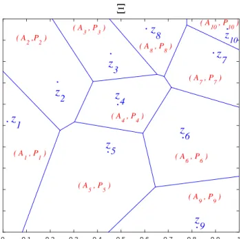
Thus, if the support of the probabilityP, say Ξ, is partitioned into a finite union of disjoint sets, Ξ = S
iAi, and Pi are the conditional probabilities given Ai, i.e.,
Pi(B) =P(B∩Ai)/pi with pi =P(Ai), and ifzi =E(Pi) are the barycenters, then
P
ipiδzi≺CXDP (see Figure 2.1 for an example).
0 0.1 0.2 0.3 0.4 0.5 0.6 0.7 0.8 0.9 1 0 0.1 0.2 0.3 0.4 0.5 0.6 0.7 0.8 0.9 1
Ξ
z
1z
4z
5z
6z
7z
2 ( A 2 ,P2 ) ( A 1 , P1 ) ( A 5 , P5 )z
9 ( A 9 , P9 ) ( A 6 , P6 ) ( A 4 , P4 ) ( A 3 , P3 )z
3z
8 ( A 8 , P8 ) ( A 7 , P7 ) z 10 ( A 10 , P10 )Fig. 2.1. Example of a partition of a 2-dimensional support Ξ of P into a finite union of
disjoint setsAisuchΞ =SiAiwith expectationE(Pi).
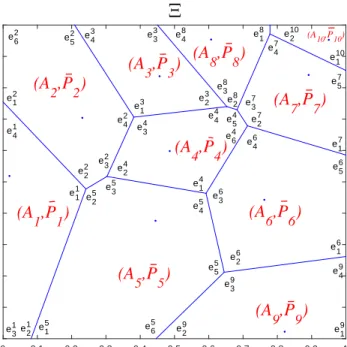
To get the inverse relation, suppose that the support of P is contained in the union of closed convex polyhedral setsAi such that their interiors are disjoint. Ai is
the convex hull of its extremal points, say{ei
1, . . . , eiKi}. Each pointuin the setAi
can be written as
(2.2) u=X
k
wki(u)eik
withwi
k(u)≥0 and
P
kw
i
k(u) = 1. If theAi’s are simplices, then the representation
in (2.2) is unique, but uniqueness is not required here (see Figure 2.2 for an example).
0 0.1 0.2 0.3 0.4 0.5 0.6 0.7 0.8 0.9 1 0 0.1 0.2 0.3 0.4 0.5 0.6 0.7 0.8 0.9 1
Ξ
e12 e62 e13 e43 e29 e24 e34 e48 e27 e42 e52 e33 e18 e57 e17 e210 e16 e56 e14 e11 e41 e39 e45 e35 e25 e22 e32 e23 e38 e47 e37 e26 e64 e28 e44 e 5 4 e46 e36 e110 e49 e19 e15 e31e21 e65 e55(A
1,P
1)
(A
3,P
3)
(A
8,P
8)
(A
7,P
7)
(A
9,P
9)
(A
6,P
6)
(A
5,P
5)
(A
2,P
2)
(A
4,P
4)
(A10,P10)Fig. 2.2. Example of a partition of a 2-dimensional support Ξ of P into a finite union of
disjoint setsAi suchΞ =SiAi with extremal points {ei1, . . . , eiki} and ¯
Pi a discrete nonnegative
measure sitting on the extremals ofAi.
Lemma 2.3. Let Piu = P kw i k(u)δei k
5 (where the weights are defined in (2.2))
and let P¯i =
´
AiP u
i dP(u), which is a discrete nonnegative measure sitting on the extremals ofAi. Notice that the barycenter ofPiu isu∈Ai. LetP¯=PiP¯i. ThenP¯ is a probability measure with the property thatP ≺CXDP¯.
Proof. Letf be convex and integrable. Then ˆ f(u)dP¯(u) =X i ˆ Ai f(u)dP¯i(u) = X i ˆ Ai X k f(eik)wki(u)dP(u) ≥X i ˆ Ai f X k wik(u)eik dP(u) =X i ˆ Ai f(u)dP(u) = ˆ f(u)dP(u).
Remark(some facts about convex order on intervals). Let the probability P be concentrated on the interval [a1, a2] and have mean µ. It is well known that the one-point lower boundP and upper boundP are
(2.3) P =δµ and P = a2−µ a2−a1 δa1+ µ−a1 a2−a1 δa2. 5As beforeδ
yis the point mass aty.
Notice that, for any affine functionf, ˆ f(u)dP(u) = ˆ f(u)dP(u) = ˆ f(u)dP(u).
One might conjecture that there may be nice lower approximations based on convex order such that equality holds even for quadratic functions, possibly by allowing the lower bound to sit on two points. The answer however is negative, as can be seen from the following example.
Example 1. LetP be the uniform distribution on [0,1]. In order that a discrete distribution in [0,1] has second moment 1/3 (as the uniform distribution) it has to sit with probability 1/2 on the points 1/2−p
1/12 and 1/2 +p1/12. Call this distribution P1. However, P1 is not dominated according to the convex stochastic sense byP, since taking the functionf(u) = (1−2u)+ we have
ˆ 1 0 (1−2u)+dP1= 0.288> ˆ 1 0 (1−2u)+dP(u) = 0.25.
One may also see that lower bounds for ´f(u)dP(u), under additional con-straints than just the expectation constraint, may depend onf. Consider the following example.
Example 2. Let the set of admissible probabilities P be discrete distributions sitting on at most three points in [0,1] such that the expectation is 1/2 and the second moment is 1/3. Denote by #(supp(P)) the cardinality of the support of P. We may show that the problem
argmin ˆ 1 0 u4dP(u) : #(supp(P))≤3, ˆ 1 0 u dP(u) = 1/2; ˆ 1 0 u2dP(u) = 1/3
has as solutionP = 1/2δa+ 1/2δ1−a witha= 1/2−
p
1/12. On the other hand, the problem argmin ˆ 1 0 −sin(u)dP(u) : #(supp(P))≤3, ˆ 1 0 u dP(u) = 1/2; ˆ 1 0 u2dP(u) = 1/3 has as a solutionP = 1/6δ0+ 2/3δ1/2+ 1/6δ1.
This means that solving the generalized moment problem as in [4, 6, 7] will give a bound for a specific fixed integrand, but not a dominating measure as in our approach. Coming back to the case of a probability P on a general interval [a1, a2], if in addition to the constraint that the expectation is µone requires that the respective lower and upper probabilitiesP andP satisfy
ˆ a2 a1 |u−µ|dP(u) = ˆ a2 a1 |u−µ|dP(u) = ˆ a2 a1 |u−µ|dP =d and ˆ a2 µ dP(u) = ˆ a2 µ dP(u) = ˆ a2 µ dP =β,
then the solution is easily found: one has to consider the subintervals [a1, µ] and [µ, a2] and find the two lower and upper bounds as in (2.3) for the two intervals and put them together for a lower bound (which then sits on two points) and an upper bound (which then sits on three points). Doing so, the lower bound is
P = (1−β)δµ− d
2(1−β) +βδµ+
d
2β,
while the upper bound is
P = d 2(µ−a1)δa1+ 1− d 2(µ−a1)− d 2(a2−µ) δµ+ d 2(a2−µ)δa2.
See Ben-Tal and Hochman [1] for the same result obtained in a different way. Notice that the refined bounds are simply obtained by dissecting the interval [a1, a2] into two subintervals [a1, µ] and [µ, a2]. Thus the refined bounds proposed in [1] appear in a natural way when the interval dissection is refined, and therefore they are included in our approach.
Remark(orderings of probability measures and risk functionals). If f is nonde-creasing and real valued, thenP ≺F SD P˜ implies that Pf ≺F SDP˜f, wherePf and
˜
Pf are the respective image measures underf. Thus, if a risk measureρis monotonic
w.r.t.≺F SD, thenP ≺F SD P˜ and u7→Q(x, u) nondecreasing for allximplies that
ρP(Q(x,·))≤ρP˜(Q(x,·)). Hence also infx ρP(Q(x,·))≤infx ρP˜(Q(x,·)).
Likewise, iff is convex and real valued, thenP≺CXDP¯ implies thatPf ≺CXD
¯
Pf, where Pf and ¯Pf are the respective image measures under f. Thus, if a risk
measure ρ is monotonic w.r.t. second-order stochastic dominance, then P ≺CXD
P0 and u 7→Q(x, u) convex and nondecreasing for all x implies that ρP(Q(x,·)) ≤
ρP¯(Q(x,·)). Hence, also infxρP(Q(x,·))≤infx ρP¯(Q(x,·)).
3. Bounding multistage stochastic optimization problems. We consider now a multistage stochastic optimization problem of the form (1.1), where the un-certainty is described by a stochastic processξ = (ξ1, . . . , ξT). This process is
char-acterized by P1, the distribution of ξ1, and the conditional distributions ξt|(ξ1 = u1, . . . , ξt−1 = ut−1) for all t > 1, denoted by Pt(·|u1, . . . , ut−1). As already men-tioned in the introduction, our goal is
(i) to find tree processes ¯P andP such that with the value functionvas in (1.1) we have
v(P)≤v(P)≤v( ¯P), or with a possible small correction term,
v(P)−≤v(P)≤v( ¯P) +;
(ii) to be able to construct refinements of these bounds by considering bushier trees, if the gap is considered too large;
(iii) to find approximate solutions for the infinite problem (1.1) based in the so-lutions of the finite problem without solving the infinite problem.
3.1. Bounds based on first-order dominance. Stochastic first-order dom-inance given in Definition 2.1 may be broken down in a multistage setting to the conditional distributions. To this end, we introduce the following definition.
Definition 3.1. We say that a process ξ is totally monotone if the conditional distributions satisfy
ξt|(ξ1=u01, . . . , ξt−1=u0t−1)≺F SDξt|(ξ1=u001, . . . , ξt−1=u00t−1)
wheneveru0
1≤u001, . . . , u0t−1≤u00t−1.6
Lemma 3.2. Let the two processesξ andξ˜be totally monotone. Let in addition
(3.1) ξt|(ξ1=u1, . . . , ξt−1=ut−1)≺F SDξ˜t|( ˜ξ1=u1, . . . ,ξ˜t−1=ut−1).
ThenP ≺F SDP˜.
Proof. Letfbe monotonic in all arguments and letPand ˜Pbe the two probability distributions associated with the totally monotone processes ξ and ˜ξ, which satisfy (3.1). Consider fT−1(u1, . . . , uT−1) := ˆ f(u1, . . . , uT)dP(uT|u1, . . . , uT−1) and ˜ fT−1(u1, . . . , uT−1) := ˆ f(u1, . . . , uT)dP˜(uT|u1, . . . , uT−1).
ThenfT−1and ˜fT−1 are monotonic in (u1, . . . , uT) and by assumptionfT−1≤f˜T−1. With a similar argument,
fT−2(u1, . . . , uT−2) := ˆ
f(u1, . . . , uT−1)dP(uT−1|u1, . . . , uT−2),
and the analogously defined ˜fT−2 are again monotonic and satisfy fT−2 ≤ f˜T−2. Continuing the integration to the end, one gets that
ˆ
f(·)dP(·)≤
ˆ
f(·)dP˜(·).
If the cost function Q(x0, ξ1, x1, . . . , ξT, xT) is monotonic in (ξ1, . . . , ξT), we can
apply Lemma (3.2) to problem (1.1) to construct upper bounds.
Example 3. Consider the following multistage stochastic optimization problem with linear constraints inx:
min ( c0(x0) +E T X t=1 ct(xt, ξt) : x∈X ) ,
6These are stronger assumptions than those introduced in the previous papers [13] and [17].
where the feasible setXis given by W0x0≥h0, A1x0+W1x1≥h1(ξ1), A2x1+W2x2≥h2(ξ2), .. . ATxT−1+WTxT ≥hT(ξT), (3.2) x1F1, .. . xT FT.
Then ifu7→ht(u) andu7→ct(xt, u) are monotonically nondecreasing, then the cost
functionQ(x0, ξ1, x1, . . . , ξT, xT) is monotonic in (ξ1, . . . , ξT). In addition, if c0 and
ct are monotonic in xand Wt are nonnegative, then Q(x0, ξ1, x1, . . . , ξT, xT) is also
monotonic inx. For later use we may also state that if (x, u)7→ct(x, u) andu7→ht(u)
are convex for all t, then the cost function Q(x0, ξ1, x1, . . . , ξT, xT) is jointly convex
in all arguments.
In the following, we elaborate the method for a three stage model; the gen-eralization to more stages can be done analogously, but the notation is more in-volved. Suppose that (ξ1, ξ2) take their values in a rectangle Ξ = [L1, U1]×[L2, U2]. Let L1 = a1 < a2 < · · · < ama+1 = U1 and, for each i = 1, . . . , ma + 1, let
L2 = bi,1 < bi,2 < · · · < bi,mb+1 = U2. Define the rectangles Ai,j = [ai, ai+1]×
[bi,j, bi,j+1], i= 1, . . . , ma, j = 1, . . . , mb. We assume that the scenario distribution
(ξ1, ξ2) has a density and therefore it does not matter that the rectangles are not disjoint. Define pi,j =P(Ai,j). Let the finite tree process ˜ξ= ( ˜ξ1,ξ2) take in each˜
rectangle Ai,j the upper value ˜ξ1 = ai+1 with probability Pjpi,j and the value on
the right ˜ξ2 =bi,j+1 with probability pi,j/Pjpi,j conditional on ˜ξ1 = ai+1. Then ˜
ξ = ( ˜ξ1,ξ˜2) := (ai+1, bi,j+1) is a finite tree process ˜P for which we solve the basic problem (1.1). Let the respective solutions be ˜xi
1 and ˜x
i,j
2 . We extend this to a decision function on Ξ by setting
˜
x1(u1) = ˜xi1 when u1∈Ai:= [ai, ai+1]
and
˜
x2(u1, u2) = ˜xi,j2 when (u1, u2)∈Ai,j.
We get v( ˜P) = ˆ Q(x0, u1,x˜1, u2,x˜2)dP˜(u1, u2) =X i,j
pi,jQ(x0, ai+1,x˜1i, bi,j+1,x˜i,j2 )
≥X i,j ˆ Ai,j Q(x0, u1,x˜i1, u2,x˜ i,j 2 )dP(u1, u2) =X i,j ˆ Ai,j
Q(x0, u1,x1(u1), u2,˜ x2(u1, u2))˜ dP(u1, u2)
= ˆ
(Q(x0, u1,x˜1(u1), u2,x˜2(u1, u2))dP(u1, u2)≥v(P).
For establishing a lower bound we use the same setup as before. Let the finite tree process ξ e = (ξ e 1, ξ e
2) take in each rectangle Ai,j the lower value ξ
e
1 = ai with
probability P
jpi,j and the value on the left ξ
e
2 =bi,j with probability pi,j/Pjpi,j
conditional on ξ e 1 =ai. Then ξ e = (ξ e 1, ξ e
2) := (ai, bi,j) is a finite tree process P
e for which we solve the basic problem (1.1). Furthermore, we have to assume that the functionQ(x0, ξ1, x2, . . . , ξT, xT) is also monotonic in thex-variables. If x∗1(u1) and x∗2(u1, u2) are the solutions of the infinite problem, we set
x+1(ai) = min u1∈Ai x∗1(u1), x+2(ai, bi,j) = min (u1,u2)∈Ai,j x∗2(u1, u2).
Since these are feasible but not necessarily optimal solutions, we get, by the assumed monotonicity, v(P) = ˆ Q(x0, u1, x∗1(u1), u2, x∗2(u1, u2))dP(u1, u2) ≥X i,j ˆ Ai,j
Q(x0, u1, x+1(ai), u2, x+2(ai, bi,j))dP(u1, u2)≥v(P
e ).
Notice that we have not only bounded the objective value, but also found an-solution for the continuous problem ifis the gap between the upper and the lower bound.
3.2. Bounds based on convex dominance. In this section we provide bounds based on convex dominance for multistage stochastic programs. One might conjecture that for two scenario processes,Pt(ut|u1, . . . , ut)≺CXDP¯t(ut|u1, . . . , ut) for alltand
all (u1, . . . , uT) is sufficient to entail P ≺CXD P¯. However this is not true, as the
following example shows.
Example 4. Let ξ1 ∼ N(0, σ21) and ξ2|ξ1 ∼N(exp(−ξ12/4), σ21). Similarly, ¯ξ1 ∼ N(0, σ22) and ¯ξ2|ξ1¯ ∼ N(exp(−ξ¯12/4), σ22). If σ1 < σ2, then ξ1 ≺CXD ξ1¯ and also (ξ2|ξ1 =x)≺CXD ( ¯ξ2|ξ¯1 =x) for all x. But (ξ1, ξ2)6≺CXD ( ¯ξ1,ξ¯2), as can be seen from the second moments ofξ2. Choose, e.g., σ1= 1/2,σ2= 1. Then
E(ξ22) =σ 2 1+ q 1/σ2 1+ 1/σ14= 4.7221>2.4142 =σ 2 2+ q 1/σ2 2+ 1/σ42=E( ¯ξ 2 2). Notice also that a convex-order dominating discrete probability cannot be found by choosing dominating discretizations for first components and for all conditional distributions of the second component and concatenating them together, as as the next example shows.
Example 5. Suppose that ξ1 is distributed according to Uniform[0,1] and that ξ2|ξ1 is distributed according to Uniform[ξ1(1−ξ1), ξ1(1−ξ1) + 1]. Let ¯ξ1 take the values 0 and 1, each with probability 1/2. Then ¯ξ1 dominates ξ1 in convex order. Likewise, for each u, let ¯ξ2(u) take the values u(1−u) andu(1−u) + 1, each with probability 1/2. Then the conditional distributionsξ2|ξ1=uare dominated by ¯ξ2(u) for all u. But, if concatenating ¯ξ1 with the conditional distributions ¯ξ2(u), only the conditional distributions foru= 0 andu= 1 are used, and one obtains that ( ¯ξ1,ξ2)¯ has a distribution that sits on all 4 edges of the unit square with equal probabilities 1/4. But this is not a convex dominant of (ξ1, ξ2), since
E(ξ22) = 16/30>E( ¯ξ 2
2) = 1/2.
The same example shows that concatenating lower bound approximations for the conditional probabilities does not lead to a lower bound approximation for the total probability. That is why, in our procedure, the full multistage sample is used to generate the bounding trees and not just the conditional distributions. Notice that this does not provide a counterexample for [11, 12], since in our exampleξ2 depends onξ1 in a very nonlinear way. On the contrary, in [11] the authors assume that the ξt are mutually independent, and the authors of [12] assume that the ξt follow an
autoregressive process (linear dependence on the past).
Again, we concentrate here on three-stage programs, noticing that the gener-alization to more stages is straightforward, but needs complicated notation. Let (ξ1, ξ2)7→Q(x0, ξ1, x1, ξ2, x2) be a convex function and letP be a probability mea-sure on a bounded rectangle inR2. Notice that the extension to
Rm×Rmis obvious,
so we omit it. As in (1.1),F1is theσ-algebra generated by the first component inR2
andF is a Borelσ-algebra ofR2. Our problem is to find (3.3) v(P) = min
x0,x1,x2E
P[Q(x0, ξ1, x1(ξ1), ξ2, x2(ξ1, ξ2))],
wherex0is deterministic,x1 is measurable w.r.t.F1, andx2 is measurable w.r.t.F. 3.2.1. Upper tree approximation based on convex-order stochastic dom-inance. Upper bounds for minimization problems are always easy to obtain, since every feasible solution constitutes an upper bound. If the basic problem P contains continuous distributions, but the approximating problem ¯P is discrete, then one has to construct a feasible solution forP out of one for ¯P. Suppose that ¯P is a scenario tree with values zi
1 in the second stage and z
i,j
2 in the third stage and ¯xi1 and ¯x
i,j
2 are its discrete solutions of the problem with ¯P as the distribution of the scenario process. Then by any reasonable extension function one may construct a solution for the continuous problem (3.3), for instance by setting
¯
x1(ξ1) = ¯xi1 ifz
i
1is the point that is closest toξ1, ¯
x2(ξ1, ξ2) = ¯xi,j2 if (z1i, zi,j2 ) is the point that is closest to (ξ1, ξ2). Obviously,
min
x0,x1(·),x2(·)
EP[Q(x0, ξ1, x1(ξ1), ξ2, x2(ξ1, ξ2))]≤EP¯[Q(x0, ξ1,x1(ξ1), ξ2,¯ x2(ξ1, ξ2))].¯ That is, any extension of a solution of any tree process ¯Pleads to a valid upper bound. However, notice that one has to evaluate the objective function for the scenario process P and the solution ¯xin order to get the value of the upper bound.
We aim, however, at finding an upper bound, which can be calculated on a finite tree without evaluating the continuous problem. A construction similar to the one for ¯P in the two-stage case may be used.
Suppose that (ξ1, ξ2) take their values in a rectangle Ξ = [L1, U1]×[L2, U2]. Let L1 = a1 < a2 < · · · < ama+1 = U1 and, for each i, let L2 = bi,1 < bi,2 < · · · < bi,mb+1 = U2 as before. Define the rectangles Ai,j = [ai, ai+1]×[bi,j, bi,j+1], i = 1, . . . , ma, j = 1, . . . , mb. We assume that the scenario distribution (ξ1, ξ2) has a density and therefore it does not matter that the rectangles are not disjoint. From now on, we use the notationei,jk for the four cornersk= 1, . . . ,4 of the rectangleAi,j,
irrespective whether these areai’s orbi,j’s.
Notice there are infinitely many ways to represent a point in a rectangle as a convex representation of the corners. However, if the rectangle represents the intervals
for the second and the third stages, we will use a product form for the weights, which implies that the weights forξ1do not depend on ξ2: let a typical rectangle be Ai,j= [ai, ai+1]×[bi,j, bi,j+1]. Then, defining as in (2.3)
wai(ξ1) = ai+1−ξ1 ai+1−ai , wai+1(ξ1) = ξ1−ai ai+1−ai ,
for ai ≤ ξ1 ≤ ai+1 one hasξ1 = wai(ξ1)ai+wai+1(ξ1)ai+1, and similarly for bi,j ≤ ξ2≤bi,j+1. Then, for (ξ1, ξ2) in the rectangleAi,j the weights are
ξ1 ξ2 =wai(ξ1)wbi,j(ξ2) ai bi,j +wai+1(ξ1)wbi,j(ξ2) ai+1 bi,j +wai(ξ1)wbi,j+1(ξ2) ai bi,j+1 +wai+1(ξ1)wbi,j+1(ξ2) ai+1 bi,j+1 . (3.4)
In general notation, denoting the four corners byei,j1 , ei,j2 , ei,j3 , ei,j4 we may equiva-lently write (ξ1, ξ2) = 4 X i=1 wei,j k (ξ1, ξ2)δei,jk .
The contribution of the probabilityP with the weights on the corners is
wki,j= ˆ
Ai,j
wei,j k
(u1, u2)dP(u1, u2).
The numerical calculation of these integrals is nearly impossible, and therefore we replace the exact calculation by a Monte Carlo integration: if (ξ(i), . . . , ξ(N)) are N replications of samples from the stochastic processξ, then the weights are defined as
wi,jk = N X n=1 wei,j k (ξ1(n), ξ2(n))1(ξ(n) 1 ,ξ (n) 2 )∈Ai,j.
LetPi,j be the distributionP conditioned on the setAi,j, i.e.,
Pi,j(D) =
1 pi,j
P(Ai,j∩D),
withpi,j=P(Ai,j) andD any measurable set. We have that
P =X
i,j
pi,jPi,j.
Let ¯Pi,j be a probability measure sitting on the extremals (the corners) ofAi,j such
that Pi,j ≺CXD P¯i,j, as is constructed in Lemma 2.3. Then P ≺CXD P¯ by the
following lemma.
Lemma 3.3. If Pi,j≺CXDP¯i,j for all i, j and
P =X
i,j
pi,jPi,j and P¯ =
X
i,j
pi,jP¯i,j,
then
P≺CXDP .¯
Proof. Letf be convex. Then EP(f) = X i,j pi,jEPi,j(f)≤ X i,j pi,jEPi,j¯ (f) =EP¯(f). ¯
P is a tree process and one may find the solution of the optimization problem on this tree. Let x∗1(eik) and x∗2(e
i,j
k ) be a solution of this problem sitting on the
nodeseik, ei,jk of the tree. We construct a continuous extension of this solution, i.e., a nonanticipative solution x∗1(ξ1) and x∗2(ξ1, ξ2) for arbitrary values of the process (ξ1, ξ2). If (ξ1, ξ2) ∈ Ai,j, then (ξ1, ξ2) = Pkw i,j k (ξ1, ξ2)e i,j k , while by construction ξ1=P kw i k(ξ1)e i k with w i k(ξ1) = P jw i,j k (ξ1, ξ2). Set ¯x1(ξ1) = P kw i k(ξ1)x∗1(eik) and ¯ x2(ξ1, ξ2) =P kw i,j k (ξ1, ξ2)x∗2(e i,j k ). By construction v( ¯P) =EP¯[Q(x0, ξ1, x∗1, ξ2, x∗2)]≥EP[Q(x0, ξ1,x¯1(ξ1), ξ2,x¯2(ξ1, ξ2))].
That is, the constructed continuous solution leads to a lower bound for the objective function. By replacing this solution with the optimal solution x∗1(ξ1), x∗2(ξ1, ξ2) of the continuous problem, we see that v( ¯P) ≥ v(P), showing that we found a valid upper bound. Notice that the constructed continuous solution is an-solution for the continuous problem, ifis the gap between the upper and the lower bound.
We finally illustrate the fact that upper bounds may be wrongly calculated when one concentrates the tree construction on conditional distributions by the following simple, but instructive, example.
Example 6. Let ξ1 be distributed according to Uniform[0,1] and let the condi-tional distributionξ2|ξ1be distributed according to Beta(0.01 + 0.36·ξ1(1−ξ1),0.3). We consider the optimization problem
(3.5) v(P) := min
x {E(ξ2−x)
2
:xis measurable w.r.t.ξ1}.
Evidently, the minimal valuev(P) is the expected conditional variance ofξ2 givenξ1, i.e.,E(V ar(ξ2|ξ1)). A numerical calculation shows thatv(P) = 0.1065. Now, finding the upper tree ˜P, given by ˜ξ= ( ˜ξ1,ξ˜2) by finding first the upper probability ˜ξ1sitting on 0 or 1 and then the upper probability ˜ξ2given that ˜ξ1= 0 or 1, results in
P( ˜ξ1= 0) =P( ˜ξ1= 1) = 0.5, P( ˜ξ2= 0|ξ1) = 0.9678,˜ P( ˜ξ2= 1|ξ1) = 0.0322.˜ However, constructing the tree ¯P, given by ¯ξ= ( ¯ξ1,ξ2) according to our method, we¯ get
P( ¯ξ1= 0) =P( ¯ξ1= 1) = 0.5, P( ¯ξ2= 0|ξ¯1) = 0.5655, P( ¯ξ2= 1|ξ¯1) = 0.4345. Solving problem (3.5) for the tree ˜P gives the valuev( ˜P) = 0.0312, whereas solving the same problem for the tree ¯P leads to the valuev( ¯P) = 0.2437. Thus, the wrong construction ˜P does not result in an upper bound, while the correct construction ¯P does.
Again notice that Example 6 does not provide a counterexample to [11, 12] since in [11] the authors assume that theξtare mutually independent, and the authors of
[12] assume that the ξt follow an autoregressive process (linear dependence on the
past).
3.2.2. Lower tree approximation based on convex-order stochastic dom-inance. The problem of finding lower bounds is slightly more involved than finding the upper bounds. We refer to the same construction of rectangles as before. Let zi,j= (zi,j
1 , z
i,j
2 ) be the barycenter ofPi,j and letPi,j=δzi,j.
By construction,Pi,j≺CXDPi,j and by Lemma 3.3,P ≺CXDP.
LetFA be theσ-algebra generated by the setsA
i,j. Notice that for all integrable
functionsf,
E[f(ξ1, ξ2)|FA] =
X
i,j
EPi,j(f)1Ai,j.
We now distinguish two cases.
• Case I. Conditionally onAi,ξ2 is independent ofξ1. • Case NI. The independence assumption is not satisfied.
Case I. In this case, the conditional expectations given Ai,j of all functions that
only depend on the first componentξ1do not depend onj; in particular,z
i,j
1 =z1i do not depend onj.
The following proposition holds true in this case.
Proposition 3.4. Let P be the tree constructed usingz1i andz
i,j
2 with scenario
probabilitiespi,j. Thenv(P)≤v(P).
Proof. Letx1(ξ1),x2(ξ1, ξ2) be a solution of the infinite problem. Then
v(P) =EP[Q(x0, ξ1, x1(ξ1), ξ2, x2(ξ1, ξ2))] =EP EP Q(x0, ξ1, x1(ξ1), ξ2, x2(ξ1, ξ2))|FA ≥EPQ x0,E(ξ1|FA),E(x1|FA),E(ξ2|FA),E(x2|FA) =EP h Qx0, z1i, x i 1, z i,j 2 , x i,j 2 i ≥v(P), where xi
1 =E(ξ1|Ai) and xi,j2 =E(ξ2|Ai,j). The last inequality comes from the fact
that we have constructed a feasible solution for P, but this need not be the optimal one. However, its optimal solution leads to a further lower bound for the problem withP as the scenario process. ThereforeP is a lower tree approximation.
CaseNI. If the independence assumption is not valid, we use a different approach.
Assumption A. Sincez7→Q(x, z) is convex and finitely valued, for every point ¯z we have
Q(x, z)≥Q(x,z) +¯ hq(¯z|x), z−z¯i,
where q(¯z|x) is a subgradient ofz7→Q(x, z) at ¯z for fixedx. We assume that there is a uniform boundC(¯z) for the norm of the subgradientsq(¯z|x), i.e.,
sup
x
kq(¯z|x)k ≤C(¯z), such thatC(ξ1) is integrable.
Under Assumption A, for all ¯ξwe have
E[Q(x, ξ)]≥E[Q(x,ξ)] +¯ Ehq( ¯ξ|x),(ξ−ξ)¯i
≥E[Q(x,ξ)]¯ −E(C( ¯ξ))·sup
ξ
kξ¯−ξk. (3.6)
The case of constraints of the form (x, z)∈B needs a little more attention. Suppose that Q(x, z) =Q0(x, z) +IB(x, z), where Q0(x, z) is convex and finitely valued and
B is a convex set.
If (x,z)¯ ∈ B and q(x,¯z) is a subgradient of z 7→ Q(x, z) at ¯z for fixed x, then Q(x, z)≥Q(x,z) +¯ hq(¯z|x), z−z¯ieven if (x, z)∈/B. Therefore (3.6) is a valid lower bound for all values ofξ.
A similar argument holds for the three-stage case: ifz1 7→Q(x0, z1, x1, z2, x2) is convex, with subgradientq(z1|x0, x1, x2, z2), then
EP[Q(x0, ξ1, x1, ξ2, x2)] ≥E[Q(x0,ξ¯1, x1, ξ2, x2)] +E[hq( ¯ξ1|x0, x1, x2, ξ2),(ξ1−ξ¯1)i] ≥E[Q(x0,ξ1, x1, ξ2, x2)]¯ −EP(C( ¯ξ1))·sup ξ1 kξ1−ξ1¯k, where ¯ξ1=E(ξ1|FA).
Notice that instead of the inequality
(3.7) E[hq( ¯ξ1|x0, x1, x2, ξ2),(ξ1−ξ1)¯ i]≤EP(C( ¯ξ1))·sup ξ1
kξ1−ξ1¯k, one could also use the inequality
(3.8) E[hq( ¯ξ1|x0, x1, x2, ξ2),(ξ1−ξ1)¯ i]≤[EP(Cp( ¯ξ1))]1/p·[EP(kξ1−ξ1¯kr)]1/r
for 1/p+ 1/r= 1.
For the construction of the lower approximating tree, as before letzi,j= (zi,j
1 , z
i,j
2 ) be the barycenters ofPi,j. However, since the lower approximation has to be a tree,
we set ¯ z1i = mb X j=1 pi,jz i,j 2 . Let P be the tree constructed using ¯zi
1 as first stage values and and z
i,j
2 as second stage values with scenario probabilities pi,j. The notation of this tree as well as of
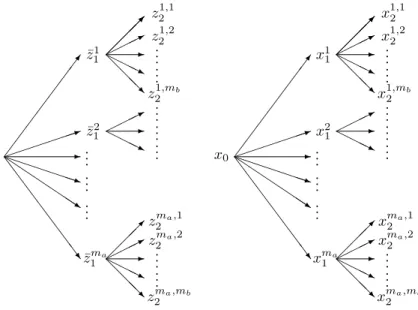
the decision tree is shown in Figure 3.1.
Proposition 3.5. LetP be the tree constructed using¯zi1as first stage values and
andzi,j2 as second stage values with scenario probabilitiespi,j. For the tree processP we have that v(P)−X i piC(¯z1i)·supkz¯ i 1−z i,j 1 k ≤v(P).
Proof. As in Proposition 3.4, we have that
EP[Q(x0, ξ1, x1(ξ1), ξ2, x2(ξ1, ξ2))] ≥EP[Q(x0, z i,j 1 , x i 1, z i,j 2 , x i,j 2 )] =EP[Q(x0,z¯1i, x i 1, z i,j 2 , x i,j 2 )] +EP[Q(x0, z1i,j, x i 1, z i,j 2 , x i,j 2 )] −EP[Q(x0,z¯i1, x i 1, z i,j 2 , x i,j 2 )] ≥EP[Q(x0,z¯1i, x i 1, z i,j 2 , x i,j 2 )]− X i piC(¯z1i)·supkz¯ i 1−z i,j 1 k. Here we have used (3.7), but alternatively one may also use (3.8).
7 1 -P P P P PPq Q Q Q Q QQs S S S S S S S w ¯ z1 1 ¯ z2 1 ¯ zma 1 .. . .. . .. . * -H HHj @ @ @ R z12,1 z12,2 z1,mb 2 * -H HHj * -H HHj @ @ @ R zma,2 1 zma,2 2 zma,mb 2 .. . .. . .. . .. . .. . .. . .. . x0 7 1 -P P P P PPq Q Q Q Q QQs S S S S S S S w x1 1 x2 1 xma 1 .. . .. . .. . * -H HHj @ @ @ R x12,1 x12,2 x1,mb 2 * -H HHj * -H HHj @ @ @ R xma,2 1 xma,2 2 xma,mb 2 .. . .. . .. . .. . .. . .. . .. .
Fig. 3.1.Left: the notation of the constructed scenario tree. Right: the pertaining decision tree.
If thezi,j1 do not coincide for different j but fixedi, then the correction term X
i
piC(¯z1i)·supkz¯i1−z
i,j
1 k,
has to be subtracted. Otherwise the correction term disappears. Notice that the correction term is small if the diameters of the rectangles are small.
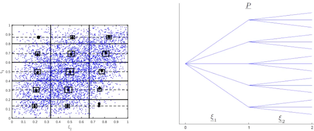
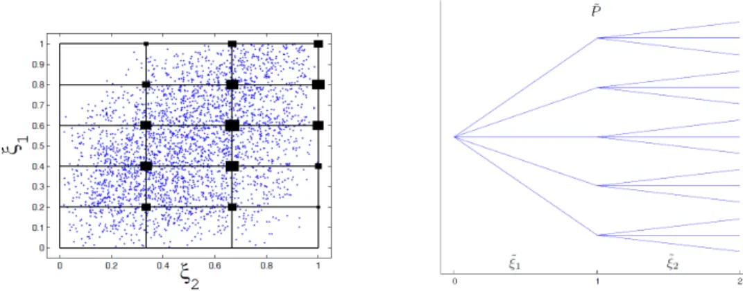
4. Lower and upper scenario trees construction: An example. In order to demonstrate the approach proposed in section 3 with a simple example, assume that the distributionP of the scenario process is given by (ξ1, ξ2), whereξ1 ∼P1 is distributed according to a Beta(2,2) distribution and ξ2|ξ1 ∼ P2(·|ξ1) is condition-ally given ξ1 distributed according to Beta(2,10..3+04−0..84··ξξ11). A sample of 5000 points distributed according toP is shown in Figure 4.1.
For given integersmaandmbwe define the setsAi,jas the rectangles with vertices
[(im−1 a, j−1 mb),( i ma, j−1 mb),( i−1 ma, j mb),( i ma, j mb)] fori = 1, . . . , ma+ 1, j = 1, . . . , mb+ 1.
The upper approximation sits on the (ma+ 1)·(mb+ 1) points (i/ma, j/mb). The
lower approximation sits on some barycenters of theAi,j. The probabilities arepi,j=
P(Ai,j).
If (u1, u2) is a point in the rectangleAi,j defined before, then letPi,j(u1, u2) be a probability measure sitting on the vertices with probability
p i−1 ma ,j−1 mb = i ma−u1 i ma− i−1 ma · j mb−u2 j mb − j−1 mb = (i−ma·u1)(j−mb·u2), p i −1 ma , j mb = i ma−u1 i ma− i−1 ma · u2− j−1 mb j mb − j−1 mb = (i−ma·u1)(mb·u2−j+ 1),
0 0.2 0.4 0.6 0.8 1 0 0.1 0.2 0.3 0.4 0.5 0.6 0.7 0.8 0.9 1
Fig. 4.1. 5000points distributed according to the distributionPof the scenario process(ξ1, ξ2),
withξ1 ∼P1 distributed according to aBeta(2,2)distribution andξ2|ξ1 ∼P2(·|ξ1)according to a Beta(2,1.4−0.8·ξ1 0.3+0.4·ξ1)distribution. 0 0.2 0.4 0.6 0.8 1 0 0.1 0.2 0.3 0.4 0.5 0.6 0.7 0.8 0.9 1 ξ2 ξ 1
Fig. 4.2. The upper approximation P¯ based on convex stochastic dominance (left) and the
corresponding scenario tree structure (right).
p i ma ,j−1 mb = u1− i−1 ma i ma− i−1 ma · j mb−u2 j mb − j−1 mb = (ma·u1−i+ 1)(j−mb·u2), p i ma , j mb = u1− i−1 ma i ma− i−1 ma · u2− j−1 mb j mb − j−1 mb = (ma·u1−i+ 1)(mb·u2−j+ 1). Notice that the expectation ofPi,j(u1, u2) is (u1, u2).
In order to estimate the upper and lower approximations ¯P andP, we use a large sample ofN random deviates (ξ(1n), ξ2(n)). Set
¯ P = 1 N N X n=1 Pi,j(ξ (n) 1 , ξ (n) 2 )·1(ξ1(n),ξ2(n))∈Ai,j. ¯
Pis a finite process, and defines a tree process, which is the upper approximation. Fig-ure 4.2 shows a construction of an upper approximation ¯P based on convex stochastic dominance with the corresponding scenario tree structure withma = 5 andmb= 3.
ξ 2 0 0.1 0.2 0.3 0.4 0.5 0.6 0.7 0.8 0.9 1 ξ1 0 0.1 0.2 0.3 0.4 0.5 0.6 0.7 0.8 0.9 1
Fig. 4.3.The barycenters (black diamonds) and the modified barycenters (black squares) of the
lower approximation tree based on convex stochastic dominance (left) and the corresponding scenario tree structure (right).
For the lower bound, the generation algorithm is a little more complicated. We sample (ξ1(n), ξ(2n)),n= 1, . . . , N, fromP and set
ni,j= 1 N N X n=1 1(ξ(n) 1 ,ξ (n) 2 )∈Ai,j, pi,j=ni,j/N, z1i,j= 1 ni,j N X n=1 ξ1(n)1(ξ(n) 1 ,ξ (n) 2 )∈Ai,j, z2i,j= 1 ni,j N X n=1 ξ2(n)1(ξ(n) 1 ,ξ (n) 2 )∈Ai,j , ¯ z1i = P jpi,jzi,j1 P jpi,j . ThenP is defined as P=X i,j pi,jδ(¯zi 1,z i,j 2 ) .
P can be represented as a tree. Arcs (i, j) for which pi,j = 0 can be
elimi-nated. Figure 4.3 shows the barycenters (z1i,j, z2i,j) (black diamonds) and the mod-ified barycenters (¯zi1, z2i,j) (black squares) for the choice ma = 5, mb = 3, and the
distribution as in Figure 4.1.
Finally Figure 4.4 shows an upper approximation ˜Pbased on first-order stochastic dominance with the corresponding scenario tree structure as described in section 3.1. Similarly, a lower approximationP
e
based on first-order stochastic dominance can be obtained by putting the weights to the left-lower corner of each rectangles in which the support has been dissected.
5. Closing the gap between upper and lower bounds. By refinement of the discretization, i.e., by letting the diameter of the boxes go to zero, we may get an arbitrarily small gap between the upper and lower bounds under the additional assumption of a growth condition. This is illustrated by the following proposition.
Fig. 4.4. The upper approximationP˜ based on first-order stochastic dominance (left) and the corresponding scenario tree structure (right).
Proposition 5.1. Suppose that the convex cost function Q satisfies the growth conditions
Q(x, z)≤Q(x,¯z) +hq(¯z|x), z−z¯i+ckz−z¯kγ
forγ >0 uniformly for all x∈X, whereq(¯z|x)is a subgradient ofz7→Q(x, z)atz¯. LetA be a closed convex polyhedron and letzAbe its barycenter underP. IfP¯ is any probability distribution whose support is contained inAand which also has barycenter
zA, then 0≤ ˆ A Q(x, z)dP(z)¯ −Q(x, zA)≤c·sup z∈A kz−zAkγ,
uniformly for all x∈X. Thus the difference between the upper and the lower bound can be controlled by making the diameter ofAsmall.
Proof. By
Q(x, z)≤Q(x, zA) +hq(zA|x), z−zAi+c· kz−zAkγ,
taking the integrals w.r.t. ¯P one gets
0≤ ˆ A Q(x, z)dP(z)¯ −Q(x, zA)≤c·sup z∈A kz−zAkγ.
Thus, by making the diameter of all boxes smaller than/c1/γ, the gap between the upper and the lower approximation will be smaller than, independently of the decisions x. Therefore the gap for the optimal values v(P)−v(P) is also smaller than.
6. Case study: A multistage production problem. This section presents a simple multistage production problem adopted to test the bounds introduced be-fore. The problem can be summarized as follows: consider a single product inventory system, which is comprised of a warehouse and a factory. The planning horizon isT periods. Random demands have to be satisfied from an inventory (the only random quantities in the model). If the random demand exceeds the stock, it will be satisfied by rapid orders from a different source, which come at a higher price. At each time step (stage), orders can be placed. The goal is to minimize the total production cost of the factory in the entire planning period.
Let us assume the following notation. Deterministic parameters:
ct is the cost of producing a unit of the product at the factory at timet= 0, . . . ,
T−1;
bt is the procurement cost from another retailer for a unit of product at time
t= 1, . . . , T;
st is the selling price at timet= 1, . . . , T;
ht is the inventory holding cost for positive inventory from time t to t+ 1,
t= 0, . . . , T−1;
d is the final value of the inventory;
Pt is the maximal production capacity of the factory at timet= 0, . . . , T −1; v0 is the amount of the product in the warehouse at the beginning of the period 1. Stochastic scenario process:
ξt is the demand for the product at timet= 1, . . . , T and all the demand must
be satisfied (the random scenario process);
ξt is the history of the demand for the product until timet. Stochastic decision variables:
xt≥0 is the amount of the product to be produced by the factory and used to satisfy
the demand at timet= 0, . . . , T −1. Auxiliary variables:
vt the amount of the product in the warehouse after sales are effectuated at
t= 1, . . . , T.
Notice that ifvtis positive,vt= [vt]+, an inventory holding costht·[vt]+will be paid to carry the stock to the next step. Ifvt is negative, vt= [vt]−, a procurement
costbt[vt]− to buy extra stock from another retailer will be paid. The final stock is
valuated with the valued[vT]+.
The problem can be modelled as follows:
minE c0·x0+h0·v0+ T−1 X t=1 ct·xt(ξt) + T−1 X t=1 ht·[vt(ξt)]++ T X t=1 bt·[vt(ξt)]− − T X t=1 st·ξt−d·[vT(ξT)]+ , (6.1) s.t. 0≤x0≤ P0, (6.2) 0≤xt(ξt)≤ Pt, t= 1, . . . , T −1, (6.3) v1(ξ1) =v0+x0−ξ1, (6.4) vt+1(ξt+1) =vt(ξt)++xt(ξt)−ξt+1, t= 1, . . . , T−1, (6.5) vt(ξt) =vt(ξt)+−vt(ξt)−, t= 1, . . . , T, (6.6) vt(ξt) +≥0, t= 1, . . . , T, (6.7) vt(ξt) − ≥0, t= 1, . . . , T. (6.8)
The objective function (6.1) denotes the expected total cost obtained from production, procurement from external retailers, and inventory holding while the last two terms are
the respective profits from selling and for the final value of the inventory. Constraints (6.2) and (6.3) impose lower and upper levels on the factory production. Finally, constraints (6.4), (6.5), (6.6), (6.7), and (6.8) define the dynamics of the inventory level and its definition.
6.1. Risk-aversion strategy: Including the average value-at-risk. Given the confidence levelα, we now introduce into model (6.1)–(6.8) the (upper) average value-at-risk: AV@Rα= min y+ 1 (1−α)E([c0·x0+h0·v0+ T−1 X t=1 ct·xt(ξt) + T−1 X t=1 ht·[vt(ξt)]++ T X t=1 bt·[vt(ξt)]−− T X t=1 st·ξt −d·[vT(ξT)]+−y]+) :y∈R , (6.9)
whereyrepresents the value-at-risk (V@R). Ifα= 0, thenAV@R0equals the expec-tation and ifα= 1, thenAV@R1 is consistently defined as the essential supremum.
Introducing the auxiliary variableu(ξT), the model (6.1)–(6.8) in a risk-aversion strategy becomes (6.10) miny + 1 (1−α)Eu(ξ T), s.t. u(ξT)≥c0·x0+h0·v0+ T−1 X t=1 ct·xt(ξt) + T−1 X t=1 ht·[vt(ξt)]++ T X t=1 bt·[vt(ξt)]−− T X t=1 st·ξt −d·[vT(ξT)]+−y, (6.11) 0≤x0≤ P0, (6.12) 0≤xt(ξt)≤ Pt, t= 1, . . . , T−1, (6.13) v1(ξ1) =v0+x0−ξ1, (6.14) vt+1(ξt+1) = vt(ξt) ++xt(ξ t)−ξ t+1, t= 1, . . . , T−1, (6.15) vt(ξt) = vt(ξt) +− vt(ξt) −, t= 1, . . . , T, (6.16) vt(ξt) +≥0, t= 1, . . . , T, (6.17) vt(ξt) −≥0, t= 1, . . . , T, (6.18) u(ξT)≥0. (6.19)
6.2. Computation of bounds for a multistage risk-averse production problem. This section presents some computational tests on the three-stage (T = 2) risk-averse production problem. We assume that the distribution P of the demand scenario process is given by ξ2 = (ξ1, ξ2), where ξ1 ∼ P1 is distributed according to a Beta(2,2) distribution andξ2|ξ1∼P2(·|ξ1) is conditionally givenξ1 distributed
Table 6.1
Production pricect, selling pricest, inventory holding costht from timetto timet+ 1, and
procurement costbt for extra stock from another retailer at timet.
t ct st ht bt
0 3.5 – 2 –
1 3.6 10.7 1.9 8
2 – 10.5 – 8.1
Table 6.2
Scenario tree structures based on first-order stochastic dominance (FSD) and convex-order dominance (CXD) adopted to compute the bounds.
Tree Number of scenarios Number of nodes
FSD-CXD T5,5 25 31 FSD-CXD T10,10 100 111 FSD-CXD T20,20 400 421 FSD T40,40 1600 1641 FSD T80,80 6400 6481 FSD T160,160 25600 25761
according to Beta(2,(1.4−0.8·ξ1)/(0.3 + 0.4·ξ1)) in the range [0,100]. The maximal production capacity of the factory at each periodt= 0,1 isPt= 567 units. The initial inventory isv0= 10, the final value of the inventory isd= 2 per unit, and the values of production price ct, selling price st, inventory holding cost ht, and procurement
costbtat time periodt are presented in Table 6.1.
The linear problems derived from our case study were solved in the AMPL en-vironment using the MOSEK solver with an interior-point algorithm. All the com-putations were performed on a 64-bit machine with 12 GB of RAM and a 2.90 GHz processor.
In order to find guaranteed bounds, we first consider two finite three-stage trees ˜ P = ( ˜ξ1,ξ˜2) andP e = (ξ e 1, ξ e
2) having the same structure T5,5: five branches from the root and five from each of the second-stage nodes resulting ink= 5×5 = 25 scenarios and 31 nodes. The two finite scenario trees have been built according to first-order stochastic dominance, as described in section 3.1, providing respective upper and lower bounds: they are obtained by dissecting the support into 25 rectangles Ai,j,
i= 1, . . . ,5,j = 1, . . . ,5, and putting the weights respectively to the left and lower corner (ai, bj) and to the up and right corner (ai+1, bj+1). Similarly, other pairs of
finite scenario trees with bushier tree structures T10,10, T20,20, T40,40, T80,80, and
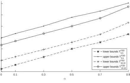
T160,160 have been considered (see Table 6.2 for details). Lower and upper bounds to the total cost of problem (6.10)–(6.19) by using the finite scenario trees based on first-order stochastic dominance (FSD) are reported in Tables 6.3, 6.4, and 6.5 and Figures 6.1 and 6.2. As expected, the worst lower and upper bounds are given by T5,5 with an absolute gap v( ˜P)−v(P
e
) of 137.5 but requiring the lowest CPU time (0.0625 CPU seconds over 30 runs). Increasing the size of the scenario tree significantly improves the bounds, monotonically reaching lower values of gaps of up to 4.11 for the biggest scenario tree considered T160,160 (see Figure 6.1 in the case of α = 0, where the bounds are plotted for increasing values of complexity of calculation measured in CPU seconds). Similar results are obtained for different values
Table 6.3
Lower bound objective function values and complexity of calculation (in CPS seconds) of finite scenario tree structures, based on first-order stochastic dominance (FSD) for increasing values ofα.
Trees v(P e ) CPU (s) α= 0 α= 0.1 α= 0.3 α= 0.5 α= 0.7 α= 0.9 TF SD 5,5 361.66 379.61 414.36 450.22 479.13 514.65 0.062 TF SD 10,10 399.09 415.49 447.27 479.49 514.06 565.42 0.078 TF SD20,20 416.66 433.89 464.34 495.87 531.56 582.08 0.093 TF SD40,40 424.98 441.91 472.85 503.94 539.45 589.18 0.156 TF SD 80,80 427.86 445.24 477.25 509.58 545.95 593.42 0.375 TF SD 160,160 430.71 448.02 479.51 511.47 547.34 596.37 3.406 Table 6.4
Upper bound objective function values and complexity of calculation (in CPS seconds) of finite scenario tree structures based on first-order stochastic dominance (FSD) for increasing values ofα.
Trees v( ˜P) CPU (s) α= 0 α= 0.1 α= 0.3 α= 0.5 α= 0.7 α= 0.9 TF SD 5,5 498.11 517.68 550.63 589.31 616.53 652.39 0.062 TF SD 10,10 466.95 484.41 517.45 550.13 585.02 636.19 0.078 TF SD 20,20 450.76 468.31 498.78 530.31 566.00 616.52 0.093 TF SD40,40 440.40 457.90 490.28 522.79 558.68 606.50 0.156 TF SD 80,80 437.88 455.18 486.54 518.54 554.38 604.34 0.375 TF SD 160,160 434.42 451.76 483.42 515.61 551.73 601.18 3.406 Table 6.5
Gaps of finite scenario tree structures based on first-order stochastic dominance (FSD) for increasing values ofα. Trees v( ˜P)v(P−v(Pe) e ) α= 0 α= 0.1 α= 0.3 α= 0.5 α= 0.7 α= 0.9 TF SD5,5 0.377 0.363 0.328 0.308 0.286 0.267 TF SD 10,10 0.170 0.165 0.156 0.147 0.138 0.125 TF SD 20,20 0.081 0.079 0.074 0.069 0.064 0.059 TF SD40,40 0.036 0.036 0.036 0.037 0.035 0.029 TF SD80,80 0.023 0.022 0.019 0.017 0.015 0.018 TF SD 160,160 0.008 0.008 0.008 0.008 0.008 0.008
of confidence levelα(see Figure 6.2). The time required to solve the problem (see last column of Tables 6.3 and 6.4) monotonically increases with the dimension of the tree, reaching the highest value for T160,160 (3.40625 CPU seconds over 30 runs). Finally, average relative gaps (v( ˜P)−v(P
e ))/v(P
e
) are reported in Table 6.5: as expected they improve monotonically with the number of scenarios in the trees, ranging from 32% for T5,5 to 0.8% for T160,160.
CPU seconds 0 0.5 1 1.5 2 2.5 3 3.5 Total Cost 360 380 400 420 440 460 480 500
Case α=0 lower bounds based on FSD
upper bounds based on FSD T5,5FSD T160,160FSD T80,80FSD T40,40FSD T20,20FSD T10,10FSD
Fig. 6.1. Lower and upper bounds on the total cost of problem (6.10)–(6.19) with confidence
levelα= 0obtained by using the finite scenario trees based on first-order stochastic dominance for increasing values of complexity of calculation measured in CPU seconds.
α 0 0.1 0.3 0.5 0.7 0.9 Total Cost 350 400 450 500 550 600 650 lower bounds T 5,5 FSD upper bounds T 5,5 FSD lower bounds T 10,10 FSD upper bounds T 10,10 FSD
Fig. 6.2.Lower and upper bounds on the total cost of problem (6.10)–(6.19)obtained by using
the finite scenario trees T5,5 and T10,10 based on first-order stochastic dominance.
We now consider lower and upper bounds built on convex stochastic dominance, as described in section 3.2. They are obtained by dissecting the support intoma×mb
rectanglesAi,j, i= 1, . . . , ma,j = 1, . . . , mb, and respectively putting the weights to
the barycenter and to the four corners. In this way the bounds can be calculated on two finite trees without evaluating the continuous problem.
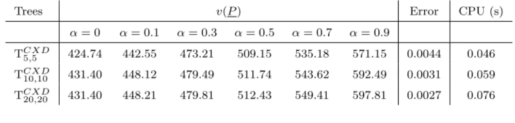
Lower and upper bounds based on convex stochastic dominance (CXD) are re-ported in Tables 6.6, 6.7, and 6.8 and Figures 6.3 and 6.4. Since ξ2 depends on ξ1,
Table 6.6
Lower bound objective function values, errorsc1Pi,jpi,j· |¯zi1−z i,j
1 |, and complexity of
cal-culation (in CPS seconds) of finite scenario tree structures based on convex stochastic dominance (CXD) for increasing values ofα.
Trees v(P) Error CPU (s)
α= 0 α= 0.1 α= 0.3 α= 0.5 α= 0.7 α= 0.9 TCXD5,5 424.74 442.55 473.21 509.15 535.18 571.15 0.0044 0.046 TCXD 10,10 431.40 448.12 479.49 511.74 543.62 592.49 0.0031 0.059 TCXD 20,20 431.40 448.21 479.81 512.43 549.41 597.81 0.0027 0.076 Table 6.7
Upper bound objective function values and complexity of calculation (in CPS seconds) of finite scenario tree structures based on convex stochastic dominance (CXD) for increasing values ofα.
Trees v( ¯P) CPU (s) α= 0 α= 0.1 α= 0.3 α= 0.5 α= 0.7 α= 0.9 TCXD5,5 436.25 454.48 484.83 520.67 575.95 621.62 0.042 TCXD 10,10 431.64 448.50 479.82 513.74 553.09 604.95 0.054 TCXD 20,20 431.40 448.21 479.81 512.43 549.41 597.81 0.078 Table 6.8
Gaps of finite scenario tree structures based on convex dominance (CXD) for increasing values ofα. Trees v( ¯Pv(P)−v(P)) α= 0 α= 0.1 α= 0.3 α= 0.5 α= 0.7 α= 0.9 TCXD5,5 0.027 0.026 0.024 0.022 0.076 0.088 TCXD 10,10 0.0005 0.0008 0.0006 0.003 0.017 0.020 TCXD 20,20 0 0 0 0 0 0
the correction term described in section 3.2.2 for lower tree approximation should be computed (see the third column of Table 6.6). This is obtained as follows: problem (6.1)–(6.8) can be rewritten as minE c0·x0+h0·v0+ T−1 X t=1 ct·xt(ξt) + T−1 X t=1 ht·[vt(ξt)]++ T X t=1 bt·[vt(ξt)]− − T X t=1 st·ξt−d·[vT(ξT)]++ Ψ[x0, . . . , xT, ξT] , where Ψ[x0, . . . , xT, ξT] = 0 if (x0, . . . , xT)∈X, ∞ otherwise,
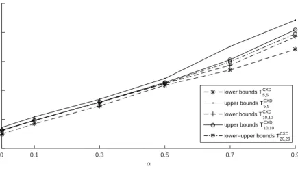
α 0 0.1 0.3 0.5 0.7 0.9 Total Cost 400 450 500 550 600 650 lower bounds T 5,5 CXD upper bounds T 5,5 CXD lower bounds T10,10CXD upper bounds T 10,10 CXD lower=upper bounds T 20,20 CXD
Fig. 6.3. Lower and upper bounds to the total cost of problem(6.10)–(6.19)obtained by using
the finite scenario trees T5,5, T10,10, and T20,20based on convex stochastic dominance (CXD).
with (6.20) X:= 0≤x0≤ P0, 0≤xt(ξt)≤ Pt, t= 1, . . . , T −1, v1(ξ1) =v0+x0−ξ1, vt+1(ξt+1) = vt(ξt) ++xt(ξ t)−ξ t+1, t= 1, . . . , T −1, vt(ξt) = vt(ξt) +− vt(ξt) −, t= 1, . . . , T, vt(ξt) +≥0, t= 1, . . . , T, vt(ξt) −≥0, t= 1, . . . , T. Let P be the tree constructed using ˜zi
1 as first stage values and and z
i,j
2 as second stage values with scenario probabilities pi,j. According to Proposition 3.5, we have
that the error made by the tree process P for our three-stage production problem by collapsing z1i,j in ¯z1i, i = 1, . . . , ma, is c1Pi,jpi,j· |z¯1i −z
i,j
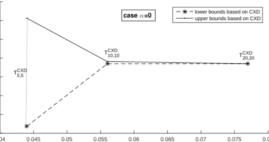
1 |. In the risk-averse case we need just to divide the previous expression by the confidence level (1−α). Notice that if the demand at time 2 is independent of the demand at time 1, then the error is null. The absolute gap between CXD lower and upper bounds based on the simplest tree structure considered T5,5reduces considerably compared to the one obtained by first-order construction, passing, in the case of α = 0, from 136.44 to 11.5 units. Increasing the size of the scenario tree to T20,20significantly improves the bounds closing the gap (see Figure 6.4) from 34.1 for FSD and taking approximately the same CPU time. Different values of confidence levelαare considered in Figure 6.3 and relative gaps (v( ¯P)−v(P))/v(P) are reported in Table 6.8: results show that the average gap reduces considerably, passing from 4% withTCXD
5,5 to 0% with T20CXD,20. 7. Conclusions. This paper develops lower and upper bounds for multistage stochastic programs based on first-order stochastic dominance and convex-order dom-inance of probability measures. The proposed method allows one to construct solu-tions for the infinite problem by considering finite tree approximasolu-tions as proxies,
CPU seconds 0.04 0.045 0.05 0.055 0.06 0.065 0.07 0.075 0.08 Total Cost 424 426 428 430 432 434 436 438
case α=0 lower bounds based on CXD
upper bounds based on CXD
T10,10CXD T
20,20 CXD
T5,5CXD
Fig. 6.4.Lower and upper bounds to the total cost of problem(6.10)–(6.19)withα= 0obtained
by using finite scenario trees based on convex dominance (CXD).
and can even be made arbitrarily close by making the approximating trees bushier. For illustration, numerical results on a multistage risk-averse production problem are presented. Results show that the solutions based on convex-order dominance con-struction outperform the ones obtained by first-order stochastic dominance, closing the gap between upper and lower bounds within a limited computational complexity and simple scenario tree structures.
REFERENCES
[1] A. Ben-Tal and E. Hochman, More bounds on the expectation of a convex function of a
random variable, J. Appl. Probab., 9 (1972), pp. 803–812.
[2] J. R. Birge, The value of the stochastic solution in stochastic linear programs with fixed
recourse, Math. Program., 24 (1982), pp. 314–325.
[3] N. Boland, I. Bakir, B. Dandurand, and A. Erera,Scenario Set Partition Dual Bounds
for Multistage Stochastic Programming: A Hierarchy of Bounds and a Partition Sampling, preprint, http://www.optimization-online.org/DB HTML/2016/01/5311.html, 2016.
[4] S. P. Dokov and D. P. Morton,Second-order lower bounds on the expectation of a convex
function, Math. Oper. Res., 30 (2005), pp. 662–677.
[5] N. C. P. Edirisinghe, Bound-based approximations in multistage stochastic programming:
Nonanticipativity aggregation, Ann. Oper. Res., 85 (1999), pp. 103–127.
[6] N. C. P. Edirisinghe and W. T. Ziemba,Bounding the expectation of a saddle function with
application to stochastic programming, Math. Oper. Res., 19 (1994), pp. 314–340.
[7] N. C. P. Edirisinghe and W. T. Ziemba,Tight bounds for stochastic convex programs, Oper.
Res., 40 (1992), pp. 660–677.
[8] Yu. Ermoliev, A. Gaivoronski, and C. Nedeva, Stochastic optimization problems with
incomplete information on distribution functions, SIAM J. Control Optim., 23 (1985), pp. 697–716.
[9] L. F. Escudero, A. Gar´ın, M. Merino, and G. P´erez,The value of the stochastic solution
in multistage problems, TOP, 15 (2007), pp. 48–64.
[10] K. FrauendorferBarycentric scenario trees in convex multistage stochastic programming,
Math. Program., 75 (1996), pp. 277–293.
[11] K. Frauendorfer and M. Sch¨urle,Multistage stochastic programming: Barycentric
approx-imation, P. Pardalos and C. A. Floudas, eds., in Encyclopedia of Optimization, Vol. 3, Kluwer Academic Publishers, Dordrecht, 2001, pp. 576–580.
[12] K. Frauendorfer, D. Kuhn, and M. Sch¨urle,Barycentric bounds in stochastic