Interval structure of Runge-Kutta methods for solving optimal
con-trol problems with uncertainties
Navid Razmjooy
Department of Electrical and Control Engineering, Tafresh University, Tafresh, 39518 79611, Iran. E-mail: [email protected]
Mehdi Ramezani∗
Department of Mathematics, Tafresh University, Tafresh 39518 79611, Iran.
E-mail: [email protected]
Abstract In this paper, a new interval version of Runge-Kutta methods is proposed for time discretization and solving of optimal control problems (OCPs) in the presence of uncertain parameters. A new technique based on interval arithmetic is introduced to achieve the confidence bounds of the system. The proposed method is based on the new forward representation of Hukuhara interval difference and combining it with Runge-Kutta method for solving the OCPs with interval uncertainties. To perform the proposed method on OCPs, the Lagrange multiplier method is first applied to achieve the necessary conditions and then, using some algebraic manipulations, they are converted to an ordinary differential equation to achieve the interval optimal solution for the considered OCP with uncertain parameters. Shooting method is also employed to cover the Runge-Kutta methods restrictions in solving the OCPs with boundary values. The simulation results are applied to some practical case studies for demonstrating the effectiveness of the proposed method.
Keywords. Optimal control, Interval analysis, Lagrange multiplier method, Runge-Kutta methods, Hukuhara
difference, Shooting method.
2010 Mathematics Subject Classification. 93Cxx, 49J30, 65G40, 65L06.
1. Introduction
Optimal control problems are generally described as deterministic problems and the coefficients in mathematic models are usually assumed as deterministic parameters when solving these models [21]. However, there are always some parameters with uncertainties which are made by different reasons, like having no exact index based on inexact coefficients in the system dynamic, neglecting some unknown parameters, unrecognized dynamics, etc. which should be considered in the performance index of the OCPs [20]. In this situation, it is clear that the results may be not well convincing for the desired control rule, or even they may give a wrong solution due to the uncertainties on the system dynamics. Therefore, the traditional methods
Received: 12 December 2017 ; Accepted: 6 April 2019. ∗Corresponding author.
can not be used for solving these problems. This problem leads researchers to utilize decision-making methods under uncertainties [33]. Recently, to cover this weakness in deterministic methods, some methods like stochastic method, fuzzy programming and interval arithmetic are proposed by considering the uncertain parameters [8,15,25]. The fuzzy and stochastic methods can be used when the probabilistic distribution and membership functions are clear. Since, if there is no information about distribution and memberships, the best way is to employ the interval method. In other words, interval optimal control problems are interesting from a theoretical point of view [26]. Interval arithmetic can be utilized for the problems with uncertainties only with some knowledge about the lower and upper bounds.
Interval methods have been introduced over the years [10]. But until 1996, the interval analysis was just summarized in simple propositions [24]. In this paper, a discrete time interval based method is proposed for solving the OCPs with interval uncertainties. Time discretization of the OCPs has been introduced since the 1960s [9]. A survey of some of the earlier works can be found in [27]. For instance, properties of Runge-Kutta methods have been analyzed in [19, 30]. Since, Runge-Kutta methods have a significant role in the numerical treatment of differential systems [16], the main purpose of our study is to propose an interval version of Runge-Kutta methods for solving OCPs with interval uncertainties. The optimal control problem in this study is
min u(t), x(t)∈∆
J(x(t), u(t),∆) = tf
Z
t0
L(t, x(t), u(t),∆)dt ,
subject to: ˙x(t) =f(t, x(t), u(t),∆), t∈(t0, tf),
x(t0) =X0,
x(tf) =Xf,
(1.1)
where,x(t) andu(t) are state and control parameters respectively, ∆ = [δ1, δ2, ..., δn] is the interval uncertainties in the system dynamic and the performance index, X0 andX1 are the initial and final states respectively and can be considered as interval integers,L(x(t), u(t),∆) =
l
−(x(t), u(t), V),¯l(x(t), u(t),∆)
is the interval-valued performance index.
This paper will propose a generalized interval based Runge-Kutta method (GIRKM) for the numerical solution of OCPs under interval uncertainties. The final results have been compared by a new introduced Euler method by Wu et. al. [34].
problem (OCP) is introduced and the methods for solving this kind of OCP is dis-cussed. Section 6 presents the numerical examples to validate the proposed IRKM for OCPs. The paper is finally concluded in section 7.
2. Interval arithmetic
In the following, the main description of the classical and the modal interval arith-metic are illustrated.
2.1. Classical Interval arithmetic. A classical definition for the interval integers over the field of real numbers can be derived as follows:
I(R) =
n
X|X = [x−,x¯]o,
X=nx|x∈R∪ {−∞,∞}, x−xx¯
o .
(2.1)
where,X is an interval integer overI(R) andx−, x¯are its lower and upper bounds,
respectively. For simplicity, in this paper, all of the interval integers are defined by uppercase symbols and bold cases will show the vector mode. Here, the intervals with the same lower and higher bounds (degenerate interval integers) are illustrated as {x} = [x, x]. The center value, width of interval number and the radius of the interval integerXcan be described as follow:
xc= 1 2
¯
x+x−, (2.2)
xw= ¯x−x−, (2.3)
xr=
xw
2 . (2.4)
Theorem 2.1. An interval integer can be described as forward and backward repre-sentation by the following definition:
X =x−+xwIF, (2.5)
X= ¯x+xwIB, (2.6)
whereIF = [0,1]andIB= [−1,0]are unit intervals.
Proof. By consideringX =hx−,x¯i:
X=x−+xwIF
xw= ¯x−x−, IF = [0, 1]
)
⇔X=x−+x¯−x−[0, 1] =hx−, x−i+h0, x¯−x−i=hx−,x¯i.
For example,X = [−1,3] : X =−1 + 4IF. By considering two interval variables
XandY, the basic arithmetic operations between them can be defined as follows:
X+Y = [+
xy¯] + [xw+yw]IB:= [x−+y−,x¯+ ¯y], (2.7)
X−Y := [x−−y,¯ x¯−y
−], (2.8)
X×Y = [¯xy¯] + [¯xyw+ ¯yxw−xwyw]IB
:= [min{xy,xy¯
−, x−y,¯ x¯y},¯ max{xy,xy¯−, x−y,¯ x¯y}¯ ],
(2.9)
X/Y =X× 1 Y,
1
Y = 1
¯
y, yw ¯
y(yw−y¯)
:= [1 ¯
y,
1
y
− ],
0∈/ [y
−,y¯].
(2.10)
More details about classic interval arithmetic can be found in [24]. Note that for multiplication and division the intervals including negative and zero integers, the interval should be first transferred into a positive interval value; in other words, we first transfer the main interval into a negative degenerate value plus a positive interval value and then the operations will be applied on them.
2.2. Modal Interval arithmetic. Modal interval method has been introduced by E. Gardens in 1985 [12]. This method can be considered as an extension of the classical intervals [11]. The main disadvantage of the classic interval arithmetic is that for any number of interval operands, when even exact arithmetic is used, the enclosure of its interval computation is often greater than a reasonably expected approximation. This issue will be made when some variables appear multiple times in the computation of the real function. For instance, considerX=[1, 3].
The ideal solution for self-differencing (X-X) and self-division (X/X ) is that these operations should have degenerate {0} and {1} values respectively. But, using the classic interval arithmetic, we have: X −X = [1,3]−[1,3] = [−2,2] and X/X = [1,3]/[1,3] =1
3,3
, respectively.
This phenomenon is calledamplification of dependence [15]. Amplification of de-pendence issue can be resolved by the modal interval analysis. In the interval analysis, by considering the condition in Eq. (2.1), the difference and division operations for two interval values likeXandYcan be achieved as follows:
X−Y =X−Dual(Y), (2.11)
where Dual
[y
−,y¯]
= [¯y, y
−] . For instance, for the example above, X −X = [1,3]−[3,1] ={0}andX/X = [1,3]/[3,1] ={1}.
More information can be achieved from [15].
3. Generalized Hukuhara (gH) Difference
Another method for compensating the amplification of dependence fordifference
operation is to utilize the H-difference. H-difference is first introduced in 1967 by Hukuhara, as a setZwhichX Y =Z ⇔X =Y +Z and the important feature of this approach was thatX X ={0} [14,17,22,23].
H-difference exists if and only if forX Y =Z,X contains a translate {Z}+Y of
Y. In 2010 Stefanini proposed a generalized version of the H-difference and called it gH-difference [31].
Definition 1. [32] Consider two interval values X and Y where X = [x−, x¯] and
Y = [y
−, y¯]. The gH-difference between these two interval sets can be defined as follows:
X gY =Z ⇔
(
(I)X =Y +Z,
(II)Y =X+ (−1)Z. (3.1)
Theorem 3.1. LetX FY be the forward representation of the gH-difference. Then
the forward representation of the gH-difference can be achieved by:
X gY =X FY =
x
−−−y
+|xw−yw|IF, (3.2)
Proof. By replacing x−, y
−,x,¯ y¯withxw, yw, xr, yr based on equations, the presented
representations can be proved.
Theorem 3.2. [15] The gH-difference for two interval integersX = [x−, x¯]and Y =
[y
−, y¯] always exists, if:
[x−, x¯] g[y−, y¯] = [z−, z¯], (3.3)
where,−z= min
x
−−y−, x¯−y¯
, z¯= max
x
−−y−, x¯−y¯
.
Proof. Refer to the reference [15]
More detailed on the gH-difference can be found in [2, 18, 31,32].
4. Generalized Interval Runge-Kutta Method for the Interval Differential Equations
(
˙
X=F(t, X,∆), atb,
X(t0) =X0.
(4.1)
where,X˙ is the Hukuhara difference of the interval integerX. ByF: [a, b]×I(Rm)×I
Rk→I(Rm) and:
F(t, X,∆) =hF−(t,X,∆),F¯(t,X,∆)i, f orX∈I(Rm),
X= [x, x], X0= [x0, x0],
(4.2)
where,X,Fand ∆ are interval vectors.
The main idea behind using the Runge-Kutta methods (RKMs) is to turn a system with initial conditions and the coefficients with real values into a differential equation. RKMs are reasonably simple and robust and can be considered as a good candidate for the numerical solution of differential equations. The main purpose of this study is to improve this method to employ it for solving equations with interval uncertainties [5].
Theorem 4.1. Consider Eq. (4.1). Let xand xbe real-valued functions such that xix¯i, i= 1,2, ..., m, and for allt∈[a, b]andF: [a, b]×I(Rm)×I Rk→I(Rm) is continuous. Let X be the interval-valued function defined by X = [x, x]. If F satisfies the Lipschitz condition,
D(F(t,X),F(t,Z))L D(X, Z),
∀(t,X)∈[a, b]×IRm. (4.3)
where g can be F and z =min{x−y, x−y}, z=max{x−y, x−y}. Consider
x
− n i
(t) =x−
i
(tn−1+h) andx− n+1 i
(t) =x−
i
(tn+h).
where, x−n i
(t) is the nth step (iteration) of the solution and h is the horizon. The
unique solution of the inclusion problem can be achieved by a generalized extension of the RKMs plus Hukuhara approach (IRKM) as follows:
(I) x−n
i
(t)x¯ni (t) :
(x
− n+1 i
(t) =x−n
i
(t) +hΦ− i
,
¯
xni+1(t) = ¯xni (t) +hΦi¯ .
(4.4)
(II) x−n
i
(t)x¯ni (t) :
x
− n+1 i
(t) =x−n
i
(t) +hΦi¯ ,
¯
xni+1(t) = ¯xni (t) +hΦ− i
. (4.5)
where for different degrees of IRKM,
GIRKM1st :
(
Φ−=−f(t, X(t),∆),
¯
GIRKM2nd:
Φ−=f−
t+h 2, X
t+h
2f(t, X(t))
,∆
,
¯ Φ =¯f
t+h 2, X
t+h
2f(t, X(t))
,∆
.
(4.7)
GIRKM4th:
Φ−= 1 6 K− 1
+ 2K−
2
+ 2K−
3
+K−
4
,
¯ Φ =1
6 ¯
K1+ 2 ¯K2+ 2 ¯K3+ ¯K4,
(4.8) where, K−
1=−f tn, X
n
(t),∆ ,
K−
2=−f
tn+h 2, X
n
(t) +
K −
1 2 ,∆
,
K−
3=−f
tn+h 2, X
n
(t) +
K −
2 2 ,∆
,
K−
4=−f
tn+h, Xn(t) +K−
3,∆
, ¯
K1=¯f tn, Xn(t),∆,
¯
K2=¯f tn+h 2, X
n
(t) + ¯
K1 2 ,∆
! ,
¯
K3=¯f tn+ h
2, X
n(t) +K¯2 2 ,∆
! ,
¯
K4=¯f tn+h, Xn(t) + ¯K3,∆.
Note that this procedure can be applied to different degrees of RKMs.
Proof. For more understanding, we prove the first order interval Runge-Kutta method (IRKM1st).
ConsiderF(t,X,∆) is a monotonic function andX∈IRm. LetX
n+1(t) be a single-ton answer of the equation with the interval real positive integer Nwith the points
{t0, t1,· · ·, tN} where tn+1 = tn +hand h= b−Na is the horizon or the same step size. By expanding the equation in [28], IRKM1st can be described by the following equation:
Xni+1(t) =Xni (t) +hF(t, Xni (t),∆). (4.9)
To get better results, we utilized H-difference for extending the formula. Here, the forward representation for H-difference is utilized (see Eq. (4.1)).
Two solutions have been achieved for Eq. (4.4). For the first term (I) x−
n+1 (t)
¯
xn+1(t):
Xni+1(t) FXni (t) =hF(t, Xni (t),∆). (4.10)
Since for the left-hand side, we have:
Xn+1(t) FXn(t) =
h
x−n+1(t)−x−n(t), x¯n+1(t)−¯xn(t)i. (4.11)
(I)
(x
−
n+1(t) =x −
n(t) +hf −(t, X
n(t),∆),
¯
xn+1(t) =¯xn(t) +h¯f(t, Xn(t),∆).
(4.12)
Repeating this method on the Eq. (4.5), on the inequality gives:
(II)
(x
− n+1
(t) =x− n
(t) +h¯f(t, Xn(t),∆),
¯
xn+1(t) =¯xn(t) +h−f(t, X n
(t),∆). (4.13)
This proof can be applied to the parts (b), (c) andIRKMnth with any order of
n.
By considering as a monotonic function, two cases arise [7]: Case 1) If the components ofF are increasing,
x
− n i
(t)¯xni (t), x− n i
(t)x¯ni (t),
(I)
x − n+1 i
(t) =x−n i
(t) +hΦ− i
,
¯
xni+1(t) = ¯x n
i (t) +hΦi¯ . (II)
x − n+1 i
(t) =x−n i
(t) +hΦi¯ ,
¯
xni+1(t) = ¯x n
i (t) +hΦ− i
.
(4.14)
Case 2) If the components ofF are decreasing,
x
− n i
(t)x¯ni (t), x− n i
(t)x¯ni (t),
(I)
x − n+1 i
(t) =x−n i
(t) +hΦi¯ ,
¯
xni+1(t) = ¯x n
i (t) +hΦ− i
. (II)
x − n+1 i
(t) =−xn i
(t) +hΦ− i
,
¯
xni+1(t) = ¯x n
i (t) +hΦi¯ .
(4.15)
The above formulations are correct if the system is monotonic. The system is monotonic if,∀xy, one hasf(x)f(y) wherefpreserve the order. If the system is not monotonic (in the critical points), the upper and the lower boundaries will be changed together; i.e. the sign of the boundaries will be changed.
5. Interval-valued optimal control problem definition
For more understanding, consider the following linear optimal control [6]:
min u(t)∈Ω=δ1×δ2
J(x(t), u(t),∆) = 1
Z
0
δ1x2(t) +u2(t)dt , (5.1)
subject to:
˙
x(t) =δ2u(t), (5.2)
where, δ1, δ2 ∈[12, 32], x(0) ={1}.
L(x,x, u, λ, t˙ ) =g(x, u, t) +λ(t)( ˙x(t)−f)
=δ1x2(t) +u2(t) +λ(t)( ˙x(t)−δ2u(t)).
(5.3)
Step 2. Apply Euler Lagrange equations to the problem and solving the equation overx(t), the following differential equation results:
x¨(t)−γx(t) = 0,
γ=δ1δ22.
(5.4)
Step 3. Apply Modal Interval Arithmetic to solve the problem: a) Compute the interval values in the problem, i.e. δ1δ22=
1 2,
3 2
3
=1 8,
27 8
,
b) Form the interval ODE systems:
x
−(t) :
¨ x(t)−27
8x(t) = 0, x(0) = 1,
¯ x(t) :
¨ x(t)−1
8x(t) = 0, x(0) = 1.
It is important to note that for simplifying the IRKMs for differential equations with order greater than 1, they first transformed into a first-order dynamic system:
x
−(t) :
˙
x1(t) =x2(t),
˙ x2(t) =
27 8x1(t), x(0) = 1,
¯
x(t) :
˙
x1(t) =x2(t),
˙ x2(t) =
1 8x1(t), x(0) = 1.
(5.5)
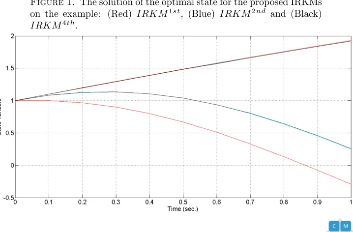
Figure 1 shows the solution of the IRKM for this example:
Figure 1. The solution of the optimal state for the proposed IRKMs
on the example: (Red) IRKM1st, (Blue) IRKM2nd and (Black)
Sometimes in optimal control, we are faced with problems with the fixed final state. Unfortunately, RKMs are designed for solving the initial value problems (IVPs). Therefore, we need an improvement to solve BVP based OCPs.
Shooting method is one of the popular methods to overcome this limitation [4, 13]. Indeed, it reduces the boundary valued problems (BVPs) to the solution of IVPs. A simple pseudo-code of single shooting method is given as follows:
1. Chooset(0)
2. Choose the step size (h) asb−a=h×N, whereN is the number of steps 3. Fork= 1,2, until convergence,do
4. i= 0, y1
0 =α, y02=t(k), z01= 0, z02= 1, 5. Fori= 0,1, , N −1,
6. Dowhileε < |t(k+1)−t(k)|, 7. CallIRKM
8. End do
The pseudo-code of the proposed method is summarized as follows:
Inputs: h,T = [a, b],
∆K = [∆,∆], (K: number of uncertainties)
Xj= [x− j
,x¯j], j= 1,2, ..., m, (m: number of states)
F(t,X(t)) Φ =f(t, Xn
i(t),∆), Outputs: X, U
Start: Apply the following operations to the interval OCP:
if OCP system is IVP: Form Lagrangian function Apply Euler Lagrange equations
Apply Interval arithmetic and generate ODE from OCP
if Xis monotonic: a)if Xis increasing Apply Eq. (4.14),
b)else-if Xis decreasing Apply Eq. (4.15),end-if end-if
else-if OCP system is BVP: Apply shooting method Return toStart end-if
end
In [34], Wu et al. introduced a simple interval Euler method to solve the ordinary differential equations which can be utilized in the OCPs. But this method has one significant restriction: the proposed method fails in solving problems governed by nonlinear differential equations.
method and interval arithmetic for improving the solution. H-difference method is also employed for covering some shortcomings of the interval arithmetic. Since the method in [34] is designed forIV P systems, another improvement based on shooting method is applied on the method for solving theBV P s.
6. Numerical Examples
In this section, the proposed method is analyzed by applying it on some case studies. The introduced case studies are taken from different sources, but we add interval uncertainties to them for analyzing the proposed IRKM.
Case study 1. Consider the following linear optimal control [1],
min u(t)∈Ω=δ1×δ2×δ3
J(x(t), u(t),∆) = 1
Z
0
δ1x2(t) +δ2u2(t)dt , (6.1)
subject to:
˙
x(t) =δ3x(t) +u(t), (6.2)
where, δ1∈[1,3], δ2∈ 1
8, 3 8
, δ3∈ 1
2, 3 2
, x(0) ={1}, x(1) = [1,1.2].
The system has interval uncertainties in both boundary condition and the index performance.
Step 1. Compute the Lagrangian function:
L(x,x, u, λ, t˙ ) =δ1x2(t) +δ1u2(t) +λ(t) ( ˙x(t)−δ3x(t)−u(t)). Step 2. Apply Euler Lagrange equations to the problem:
˙
x(t)−δ3x(t)−u(t) = 0,
2δ2u(t)−λ= 0,
2δ1x(t)−δ3λ−λ˙ = 0.
Step 3. By solving the equation above over , the following differential equation results:
¨
x(t)−γx(t) = 0,
γ=δ1 δ2
+δ23,
Step 4. Apply Modal Interval Arithmetic to solve the problem:
a) Compute the interval values in the problem,
δ1
δ2
=δ1×
1 Dual(δ2)
=
3 8
,
δ23=
1 4,
9 4
,
→γ= δ1
δ2 +δ 2 3=58,
21 8
.
b) Form the interval ODE systems:
x
−(t) :
¨ x(t)−21
8x(t) = 0, x(0) = 1, x(1) = 1.2.
, x¯(t) :
¨ x(t)−5
8x(t) = 0, x(0) = 1, x(1) = 1.
x
−(t) :
˙
x1(t) =x2(t),
˙ x2(t) =
21 8x1(t), x(0) = 1,
x(1) = 1.2,
¯ x(t) :
˙
x1(t) =x2(t),
˙ x2(t) =
5 8x1(t), x(0) = 1,
x(1) = 1.
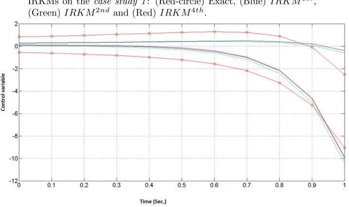
Solving the interval ordinary differential equation by the proposed IRKM results:
Figure 2. The solution of the optimal state for the proposed IRKMs
on the case study 1: (Red-circle) Exact, (Blue)IRKM1st, (Green)
IRKM2nd and (Red)IRKM4th.
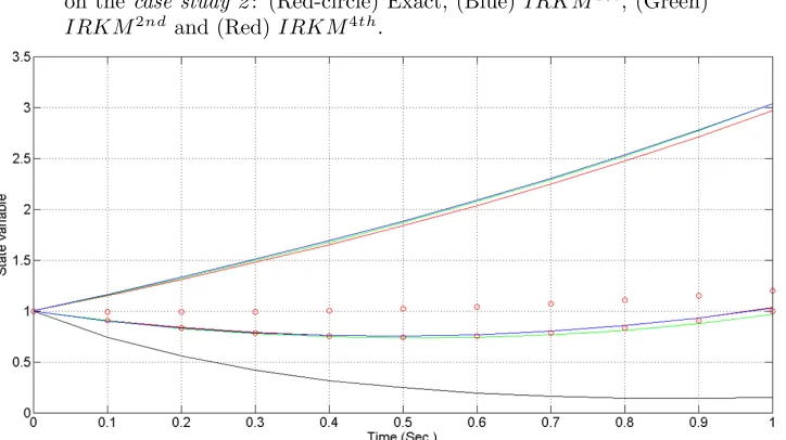
From the Figure 2, it is clear that by increasing the order of IRKM, the results get closer to the answer. For more analyzing and comparing the IRKMs, we put the results in Table 1 and finally with an intervalL−2 norm, the results are compared. The interval L-2 norm for two interval integersX andY are formulated as follows:
kX−Yk2=q(x−y)2+ (x−y)2, (6.3)
T able 1. Comparison of the IRKMs and Exact v alues for optimal con trol u ∗ ( t ). Time E xactM ethod I R K M 1 s
t[34
From the Table 1, it is clear that as the order of the IRKM increases, the error reduces. Here, the exact method is simulated by the hybridIRKM4thandIRKM5th. Case study 2. Consider the following tracking optimal control problem where the dynamical system is nonlinear and the performance index is quadric [3].
min u(t)∈Ω=δ1×δ2
J(x(t), u(t),∆) = 1
Z
0
(δ1−x(t)) 2
+u2(t)dt, (6.4)
subject to:
˙
x(t) =−δ2
p
x(t) +u(t), (6.5)
where, δ1∈[1,3], δ2∈[−1,−0.25], x(0) ={0}, x(1) = 1
2, 3 2
.
After performing the initial operations, the interval ODE systems is obtained as follows:
x
−(t) :
˙
x1(t) =x2(t),
˙
x2(t) =x(t)−
3 4x1(t), x(0) = 0,
x(1) = 1,
¯
x(t) :
˙
x1(t) =x2(t),
˙
x2(t) =x(t)−
191 64x1(t), x(0) = 0,
x(1) = 3.
(6.6)
Solving the interval ordinary differential equation by the proposed IRKM results the following solution:
Figure 3. The solution of the optimal state for the proposed IRKMs
on the case study 2: (Red-circle) Exact, (Blue)IRKM1st, (Green)
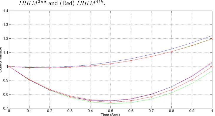
Figure 4. The solution of the optimal control for the proposed
IRKMs on the case study 1: (Red-circle) Exact, (Blue) IRKM1st, (Green)IRKM2nd and (Red)IRKM4th.
Different orders of IRKMs are applied on the system and are compared with the exact value. As it can be seen from the Figure 3 and Figure 4, the interval bound is improved by increasing the order of IRKM.
7. Conclusions
This paper has proposed a new robust topology for the optimal control problems with uncertain-but-bounded parameters (i.e. parameters which are described by an interval with lower and upper bound). The proposed method is an extension of Runge-Kutta method based on interval arithmetic. Interval analysis theory and its extension approaches including generalized Hukuhara method are employed to im-prove the proposed method. The proposed method is described by a new description which is called forward representation. The main purpose of the proposed method is to determine interval optimal control and state vector of the optimal control problems with interval uncertainties by a direct method of solution based upon an improved version of Runge-Kutta method. The numerical examples show that one of the su-periorities of the proposed interval method over the Euler method is its efficiency, especially when the range and number of uncertain variables are large.
References
[1] A. Akkouche, A. Maidi, and M. Aidene, Solving optimal control problems by variational ap-proach based on the Adomian’s Decomposition Method, in Proc. In Systems and Control (ICSC), 2013 3rd International Conference on, (2013), 218–223.
[3] S. Berkani, F. Manseur, and A. Maidi,Optimal control based on the variational iteration method, Comp. & Math. with Apps.,64(4) (2012), 604–610.
[4] H. Bock, M. Diehl, D. Leineweber, and J. Schlder,A direct multiple shooting method for real-time optimization of nonlinear DAE processes, Nonlinear Model Predictive Control, 2000, 245– 267.
[5] C. Bresten, S. Gottlieb, Z. Grant, D. Higgs, D. Ketcheson, and A. Nmeth, Explicit strong stability preserving multistep Runge–Kutta methods, Math. of Comp.,86(304) (2017), 747–769. [6] D. N. Burghes and A. Graham,Introduction to control theory, including optimal control, 1980. [7] Y. Chalco-Cano and H. Romn-Flores,On new solutions of fuzzy differential equations, Chaos,
Solitons Fractals,38(1) (2008), 112–119.
[8] L. Chen and S. S. Rao,Fuzzy finite-element approach for the vibration analysis of imprecisely-defined systems, Finite elements in analysis and design,27(1) (1997), 69–83.
[9] A. Dontchev and W. Hager, The Euler approximation in state constrained optimal control, Math. of Comp.,70(233) (2001), 173–203.
[10] W. Edmonson and G. Melquiond, IEEE Interval Standard Working Group-P1788: Current Status, In Computer Arithmetic 19th IEEE Symposium on, (2009), 231–234.
[11] A. Elskhawy, K. Ismail, and M. Zohdy,Modal interval floating point unit with decorations, InBook of Abstracts, 2014, 49.
[12] E. Gardees, H. Mielgo, and A. Trepat,Modal intervals: reason and ground semantics, in Interval Mathematics 1985, ed. Springer, 1986, 27–35.
[13] F. Geng and Z. Tang,Piecewise shooting reproducing kernel method for linear singularly per-turbed boundary value problems, Applied Mathematics Letters,62(2016), 1–8.
[14] L. T. Gomes and L. C. Barros,A note on the generalized difference and the generalized differ-entiability, Fuzzy Sets and Sys.,280(2015), 142–145.
[15] N. Razmjooy and M. Ramezani,Solution of the Hamilton jacobi bellman uncertainties by the interval version of adomian decomposition method, Int. Rob. Auto. J.,4(2) (2018), 113–117. N. T. Hayes, Introduction to modal intervals, available at grouper, ieee. org/groups/1788/Material/Hayes ModalInterval. pdf, 1788.
[16] M. Herty, L. Pareschi, and S. Steffensen,Implicit-explicit Runge–Kutta schemes for numerical discretization of optimal control problems, SIAM J. Num. Analysis,51(4) (2013), 1875–1899. [17] M. Hukuhara,Integration des applications mesurables dont la valeur est un compact convexe,
Funkcial. Ekvac,10(1967), 205–223.
[18] E. Hllermeier,An approach to modelling and simulation of uncertain dynamical systems, Int. J. Uncertainty, Fuzziness and Knowledge-Based Sys.,5(2) (1997), 117–137.
[19] C. Y. Kaya, Inexact restoration for RungeKutta discretization of optimal control problems, SIAM J. Num. Analysis,48(4) (2010), 1492–1517.
[20] N. Razmjooy and M. Ramezani,Uncertain Method for Optimal Control Problems With Uncer-tainties Using Chebyshev Inclusion Functions, Asian J. Control, 2019.
[21] U. A. S. Leal, G. N. Silva, and W. A. Lodwick,Necessary condition for optimal control problem with interval-valued objective function, Proc. Series of the Brazilian Soc. of Comp. and App. Math.,3(1) (2015), 010131–7.
[22] V. Lupulescu,Hukuhara differentiability of interval-valued functions and interval differential equations on time scales, Info. Sci.,248(2013), 50–67.
[23] M. T. Malinowski,Interval Cauchy problem with a second type Hukuhara derivative, Info. Sci.,
213(2012), 94–105.
[24] R. E. Moore, R. B. Kearfott, and M. J. Cloud,Introduction to interval analysis, Society for Industrial and Applied Mathematics, SIAM, 2009.
[25] I. Narayanan, D. Wang, A. Sivasubramaniam, and H. K. Fathy,A Stochastic optimal control approach for exploring tradeoffs between cost savings and battery aging in datacenter demand response, IEEE Trans. Control Sys. Tech., 2017.
[26] O. V. Olegovna,Interval optimal control problem in a Hilbert space, Computational Math. and Mathematical Phys.,53(4) (2013), 389–395.
[28] D. Ravat,Analysis of the Euler method and its applicability in environmental magnetic inves-tigations, J. Environmental and Eng. Geophysics,1(3) (1996), 229–238.
[29] S. Salahshour and M. Khan,Exact solutions of nonlinear interval Volterra integral equations, Int. J. Ind. Math.,4(4) (2012), 375–388.
[30] J. Sanz-Serna,Symplectic Runge–Kutta schemes for adjoint equations, Auto. Differentiation, Optimal Control, and More, SIAM Review,58(1) (2016), 3–33.
[31] L. Stefanini,A generalization of Hukuhara difference and division for interval and fuzzy arith-metic, Fuzzy sets and sys.,161(11) (2010), 1564–1584.
[32] L. Stefanini and B. Bede, Generalized Hukuhara differentiability of interval-valued functions and interval differential equations, Nonlinear Analysis: Theory, Methods Applications,71(3) (2009), 1311–1328.
[33] N. Razmjooy and M. Ramezani,Robust optimal control of two-wheeled self-balancing robot using Chebyshev inclusion method, Majlesi j. Elec. Eng.,12(1) (2018), 13–21.
J. Wu,Uncertainty analysis and optimization by using the orthogonal polynomials, 2015. Thesis (Ph.D.).